Bayesian Risk Aggregation: Correlation ... - ERM Symposium

Bayesian Risk Aggregation:
Correlation Uncertainty and Expert Judgement
Klaus Böcker ∗ Alessandra Crimmi † Holger Fink ‡
Abstract
In this paper we present a novel way for estimating aggregated EC figures based
on Bayesian copula estimation. Contrary to the classical approach of using a single
(point estimator) inter-risk-correlation matrix we derive a probability distribution of
possible correlation matrices that enables us to tackle the important issue of param-
eter uncertainty. More precisely, we describe in detail how formal expert judgement
can be performed and utilised to augment scarce empirical, resulting in a posterior
distribution that contains all relevant information about the inter-risk-correlation
matrix. We then present simulation algorithms based on Markov-Chain-Monte-Carlo
methods that allow to simulate sample correlation matrices from different posterior
distributions. Finally, we give a numerical example that serves to illustrate our new
approach and, in particular, shows how important accuracy measures for aggregated
economic capital and diversification benefits can be obtained by adopting a Bayesian
perspective.
1 Introduction
The 2007/2008 global financial crisis has demonstrated serious weaknesses in corporate
governance and risk management, in particular, many institutions’ lack of ability to create
a viable and sound framework for risk appetite. In addition to design failures such as
disregarding funding risk and the liquidity risk in trading portfolios, risk managers focused
too much on single number metrics like value-at-risk (VaR) or economic capital (EC)
instead of using a number of distinct risk measures.
∗Risk Analytics and Methods, UniCredit Bank AG, München, Germany,
email: klaus.boecker@unicreditgroup.de
† Risk Analytics and Methods, UniCredit Group, Milan, Italy,
email: alessandra.crimmi@unicreditgroup.eu
‡ Center for Mathematical Sciences, Munich University of Technology, Garching bei München,
Germany, email: fink@ma.tum.de
1

Economic Capital [EUR mn] Dec 31, 2009
Market risk 3, 564
Credit Risk 9, 981
Operational risk 2, 612
Business risk 1, 666
Total EC 17, 823
Table 1.1: Prototypical example of a bank’s Pillar 3 report of EC for different risk types as well as the
aggregated EC. Given no further information about the measurement error, the presented number for
aggregated EC suggests an absolute uncertainty of ±1 mn EUR, corresponding to a relative uncertainty
of 0.0056 %.
Assessing risk by means of a single number only becomes even more of a problem
if quantitative mathematical models are used without any adjustment for model uncer-
tainty. Much too often in risk management practices, results are calculated to a fictitious
degree of accuracy, which is greater than is warranted by the data used in the calculation.
As a typical example, look at the—of course illustrative but nevertheless realistic—EC
figures for different risk types and total aggregated EC presented in Table 1.1. Recall
that the purpose of EC is to capture extreme losses and therefore it is measured at high
confidence levels typically in a range between 99.50 % and 99.98 %. The way the figures
are presented in Table 1.1 suggests that the aggregated EC, which is a key element in the
practical implementation of a bank’s risk appetite framework has been determined with
the incredible relative precision 1 of ±5.6 × 10 −5 .
Such pseudo accuracy leads to a wrong subjective risk perception and may create a
dangerous overconfidence of the decision maker. In general, the feeling of greater security
tempts people to be more reckless and, in the context of risk management, leads deci-
sion makers to concentrate mainly on the upside opportunity of markets and to neglect
downside risk. One of the main concerns in connection with risk aggregation is of whether
and to which extent diversification benefits between different risk types can be identified.
Apart from the very simple approach of adding-up all EC estimates for each risk category
or business line one can distinguish between top-down or modular approaches on the one
hand and bottom-up or multi-factor simulation approaches on the other, cf. for instance
Saita [24] for further information and references about principles of risk aggregation.
Bottom-up approaches basically model all the bank’s real and financial variables in-
cluding assets, liabilities and interest sensitive off-balance sheet items simultaneously, see
for e.g. Kretzschmar, McNeil, and Kirchner [16]. This allows to capture gains and losses at
1 As an illustration, the same relative error is obtained when computing a distance of about 18 meters
while maintaining an accuracy of 1 mm.
2

the level of individual instruments or positions without the need for creating artificial risk
silos. Such sophisticated approaches are particularly important for market and credit risk,
which are highly related and inextricably linked with each other, see e.g. the Research
Task Force of the Basel Committee on Banking Supervision [2] and Hartmann, Pritsker,
and Schuermann [14] for more about the interaction of market and credit risk.
While financial institutions and supervisors are seeking for flexible bottom-up methods
for the aggregation of market and credit risk, conceptual difficulties remain with respect
to other risk types such as operational risk and business risk. As a matter of fact, banks
are currently still favoring simpler top-down methods when computing their aggregated
EC as pointed out in IFRI/CRO Forum [15]. According to this survey the most popular
method in practice is the aggregation-by-risk-type approach where stand-alone risk figures
of different risk types are combined in some way to obtain the desired aggregated EC. In
a similar, more recent survey of the Basel Committee [3] it is reported that “there is no
established set of best practices concerning risk aggregation in the industry.” From all this,
it can be expected that for quite a long time hybrid approaches that at least partially rely
on an inter-risk-correlation matrix, will heavily influence market practices.
The simplest form of risk aggregation expresses the dependence between different risk
types by an inter-risk-correlation matrix R, and its estimation and calibration is a core
problem for the calculation of total EC in practice. A standard approach is to model the
dependence structure between risk types by a distributional copula, see e.g. the references
in Böcker [5]. Estimates for inter-risk-correlations differ significantly within the industry.
The IFRI/CRO Forum [15] points out that“correlation estimates used vary widely, to
an extent that is unlikely to be solely attributable to differences in business mix.” This
obviously shows that the estimation of inter-risk correlations is afflicted with high uncer-
tainties. One reason for this is that very often reliable data are scarce and do not cover
long historical time periods. Therefore, inter-risk correlations are approximated by the co-
movement of asset price indices or similar proxies of which, it is hoped, are representative
for these risk types. As a consequence thereof, a reliable and robust statistical estimate of
the inter-risk-correlation matrix is often not possible and it is necessary to draw on expert
opinions. This has recently also been acknowledged by the Committee of European Bank-
ing Supervisors in their recent consultation paper [8], where they explicitly distinguish
statistical techniques versus expert judgements.
Our work makes two novel contributions for estimating aggregated EC within an
aggregation-by-risk-type framework. First, we explicitly address the existence of param-
eter uncertainty associated with the inter-risk-correlation matrix. Second, we present a
sophisticated method for assessing inter-risk correlations (more precisely, the Gaussian
copula parameters) by means of expert judgement. To illustrate our approach, we calcu-
3

late aggregated EC for the same sample portfolio already used in Böcker [5], consisting
of 10 % market risk, 61 % credit risk, 14 % operational risk, and 15 % business risk in
terms of 99.95 % EC. Here, however, we make an assumption which is key to what fol-
lows, namely that as a consequence of all the uncertainties a bank’s inter-risk-correlation
matrix cannot be considered as a fixed parameter of the risk-aggregation model but should
rather be treated as a random parameter. Hence, the inter-risk-correlation matrix R (or,
more generally, the parameters of the copula) is described by a distribution function,
which is referred to as the posterior distribution. This distribution comprises information
stemming from empirical data X (e.g. time series of risk proxies representative for each
risk type) as well as from expert judgement.
This paper is organised as follows. In Section 2 we will briefly recap the “classical”
aggregation-by-risk-type approach using a fixed Gaussian copula and also introduce the
portfolio that serves as an illustrative example. Section 3 then describes the construction of
the prior and posterior distribution of the inter-risk-correlation matrix by considering the
different pair correlations separately. For two specific models (the beta and the triangular
models) we suggest a Markov-Chain-Monte-Carlo (MCMC) algorithms that can easily be
used to sample a set of correlation matrices from the posterior. In Section 4 we discuss a
numerical example of risk aggregation and, finally, Section 5 is devoted to the important
issue of how inter-risk correlations may be estimated using expert knowledge.
2 Classical copula aggregation
A d-dimensional distributional copula C is a d-dimensional distribution function on [0, 1] d
with uniform marginals. Among all copulas discussed in the literature, maybe those most
frequently used for risk aggregation are the Gaussian copula and the t copula. The impor-
tance of copulas for financial risk management is essentially a result of Sklar’s theorem,
stating that every multivariate distribution function can be separated into their marginal
distribution functions and a copula. Therefore, copulas allow for a separate modelling of
the marginal distribution functions of distinct risk types on the one hand and their depen-
dence structure (i.e. the copula) on the other. Distributional copulas have been frequently
applied to risk aggregation e.g. Dimakos & Aas [9], Rosenberg & Schuermann [23], Ward
& Lee [26], or Brockmann & Kalkbrener [6].
In the sequel, we summarise some properties of the Gaussian copula, see Cherubini,
Luciano, and Vecchiato [7] for more details. Let Φ denote the standard univariate normal
distribution function, Φ d R
the standard multivariate normal distribution function with
d × d correlation matrix R, and (u1, . . . , ud) ∈ [0, 1] d . Then, the distribution function of
4

the d-dimensional Gaussian copula is given by
C d R(u1, . . . , ud) = Φ d R(Φ −1 (u1), . . . , Φ −1 (ud)) (2.1)
where Φ −1 (·) denotes the inverse of the standard normal distribution function. The density
of the d-dimensional Gaussian copula can be written as
c d 1
−
R(u1, . . . , ud) = det(R) 2 exp
with ξ = (Φ −1 (u1), . . . , Φ −1 (ud)) ′ and identity matrix Id.
− 1
2 ξ′ (R −1 − Id)ξ
(2.2)
We now turn to the estimation of the Gaussian copula which is usually done by
maximising the corresponding likelihood function. Suppose x1, . . . , xn is an n-sample of
d×1 mutually independent observations that are identically distributed. In the context of
inter-risk aggregation each marginal component of xj, j = 1, . . . , n, represents a suitable
risk driver or loss proxy representative for a different risk type. Specifically, assuming a
Gaussian copula model means that all components of xj, j = 1, . . . , n, have a Gaussian
dependence structure.
After transforming the sample data xj into variates uj with uniform marginals (e.g.
using order statistics or parametric distribution functions), we obtain for the likelihood
of the Gaussian copula
1
−
l(R|ξ1, . . . , ξn) ∝ det(R) 2 n exp
− 1
2 tr(R−1
B) . (2.3)
Here, the d×d symmetric, positive semidefinite matrix B is the sample covariance matrix
of the data after transformation to standard Normal marginals, i.e.
B = 1
n
n
j=1
ξ jξ ′
j with ξ j = (Φ −1 (u1j), . . . , Φ −1 (udj)) ′ , (2.4)
which is also the global maximum of the likelihood function (2.3), see e.g. Press [20], p.
183. Without loss of generality, we may always use a standardised sample ξ j that has
exactly unit sample variance so that B equals the sample correlation matrix. Then we
finally obtain the MLE of the Gaussian copula parameter as
ˆR = 1
n
n
j=1
ξ jξ ′
j .
After the matrix ˆ R has been determined, one can start risk-type aggregation. As men-
tioned in the introduction, we adopt the portfolio used in Böcker [5] consisting of 10 %
market risk, 61 % credit risk, 14 % operational risk, and 15 % business risk, representing
5

Risk Distribution function Parameters
MR F (x) = Fν , x ∈ R µ = 0, σ = 2.18, ν = 10
x−µ
σ
CR F (x) = X = 2338.64,
Φ √
√ϱ
1
−1 x
1 − ϱ Φ ( X ) − Φ−1 (p) , x > 0 p = 0.3%, ϱ = 8%
OR F (x) = Φ ln x−µ
σ
BR F (x) = Φ x−µ
σ
, x > 0 µ = −0.893, σ = 1.089
, x ∈ R µ = 0, σ = 4.56
Table 2.2: Marginal distributions for market risk (MR), credit risk (CR), operational risk (OR), and
business risk (BR), where Fν is the Student-t distribution function with ν degrees of freedom and Φ
is the standard normal distribution function. MR follows a scaled Student-t and CR is described by a
Vasicek distribution with total exposure X, uniform asset correlation ϱ, and average default probability
p. Operational risk (OR) is assumed to be lognormally distributed and business risk (BR) is modelled
by a normal distribution. The parameters for the distribution functions are chosen so that MR, CR, OR,
and BR absorb 10, 61, 14, and 15 units of EC at 99.95 % confidence level. Finally, only credit risk and
operational risk have non-zero expected losses of about 7.0 and 0.7, respectively.
an industry average obtained from large banks reported in IFRI/CRO Forum [15], Fig-
ure 16. Furthermore, we assume that EC for each risk type was calculated at confidence
level of 99.95 %, time horizon of one year, and that the marginal distribution functions are
as in Table 2.2. Now, assuming that the inverses F −1
i (·), i =, 1, . . . , d, of all marginal risk
type distribution functions Fi(·) exist, classical risk aggregation with a Gaussian copula
is straight-forward. In a first step, one simulates a large number N of mutually indepen-
dent d × 1 vectors u1, . . . , uN from the Gaussian copula C d ˆ R . Note that by definition for
all j = 1, . . . , N the marginal components {u1j, . . . , udj} of the vectors uj are uniformly
distributed with a Gaussian dependence structure. In a second step, all marginal components
are transformed according to F −1
i (uij), i = 1, . . . , d, j = 1, . . . , N. Since copulas
are invariant under strictly increasing transformations, the dependence structure between
{F −1
1 (u1j), . . . , F −1
d (udj)}j=1,...,N is the same as between {u1j, . . . , udj}j=1,...,N, that is a
Gaussian one. Finally, a simulated N-sample of aggregated EC can be computed through
d −1
i Fi (uij)
j=1,...,N .
3 Bayesian risk aggregation
3.1 Construction of the inter-risk-correlation prior
In the Bayesian approach for risk-type aggregation, one has to find a suitable prior for the
inter-risk-correlation matrix R of the Gaussian copula. This prior quantifies the available
6

expert knowledge regarding the inter-risk-correlation matrix in probabilistic form. Since
our example portfolio consists of d = 4 risk types, it is sufficient to consider 4×4 correlation
matrices R, which can be identified with a 6-dimensional real vector by
⎛
⎞
⎜
R = ⎜
⎝
1 r1 r2 r3
· 1 r4 r5
· · 1 r6
· · · 1
⎟
⎠ ←→ (r1, r2, r3, r4, r5, r6), ri ∈ [−1, 1], 1 ≤ i ≤ 6. (3.1)
The most commonly used prior model for a covariance matrix Σ is the inverse-Wishart
distribution, see e.g. Press [20]. Since every covariance matrix Σ is related to a correlation
matrix R by
Σ = S 1/2 R S 1/2 , (3.2)
where S = diag(σ11, σ22, . . .) and σjj are the diagonal elements of Σ, the inverse-Wishart
prior can also be used to construct a prior for the correlation matrix.
The inverse-Wishart-based prior for the inter-risk-correlation matrix allows only for
one single degrees of freedom parameter ν to express prior beliefs (and thus the level of
uncertainty) about R. In practice, however, the amount of available expert information
for different pair correlations ri, i = 1, . . . , 6, may significantly depend on the risk-type
combinations. Another drawback of the inverse-Wishart distribution is that the resulting
prior for R cannot easily be estimated by means of expert judgement. Note, that the
prior distribution for R is calculated from the inverse-Wishart prior for Σ through trans-
formation (3.2), which rarely yields a prior distribution that can easily be specified by
expert elicitation. All this leads to the conclusion that the inverse-Wishart based prior is
inadequate for our purpose and that we have to construct a more flexible prior for R.
Thus we have decided to use a kind of “bottom-up” approach when building the prior
distribution for the inter-risk-correlation matrix. In a first step, prior information for each
component ri, i = 1, . . . , 6, of R is separately modelled by one-dimensional distributions
with Lebesgue densities πi(ri), i = 1, . . . , 6. This yields a distribution of symmetric, real-
valued matrices with diagonal elements equal to one. In a second step we restrict to
those matrices preserving the positive semidefiniteness of the correlation matrix. Hence,
denoting the space of all 4-dimensional correlation matrices by R 4 , a possible density for
the correlation matrix prior can be written as
π(R) =
πi(ri) 1 {R∈R4 }. (3.3)
1≤i≤6
The indicator function 1{·} ensures that the matrices are positive definite and thus are
proper correlation matrices, and also introduces a dependence structure among the ri for
i = 1, . . . , 6.
7

Pairwise correlation priors As we describe in more detail in Section 5, a well-
established approach for the subjective determination of a prior density is by matching a
given functional form. The shape of the prior reflects the amount and the quality of the
available information and should match the experts’ beliefs as closely as possible.
As risk managers are concerned about unreasonable and possibly incorrect diversifi-
cation benefits, it is normally assumed that correlations between different risk types are
non-negative. Such a boundary condition for the correlation matrix can easily and natu-
rally be modelled within the Bayesian framework by considering only pairwise priors πi
that have support in [0,1].
Example 3.1. [Uniform prior]
Assume that the experts are totally uninformed about the possible values of the single
pair correlations ri for i = 1, . . . , 6. Consequently, we may want to take all values of ri as
equally likely and, in consideration of the general restriction ri ∈ [0, 1], a natural diffuse
prior is the uniform distribution
πi(ri) ∝ 1{0

Example 3.3. [Triangular distributed prior]
An alternative family of useful prior distributions for a correlation parameter is the sym-
metric triangular distribution giving values between αi and βi with −1 ≤ αi < βi ≤ 1.
Then, the prior density for all ri, i = 1, . . . , 6, is of the form
T (ri|αi, βi) = 4 βi − ri
(βi − αi) 2 1{(αi+βi)/2

Gibbs sampling One possibility is to simultaneously simulate a 6-dimensional Markov
chain of the vector of pair correlations (r1, . . . , r6), e.g. by using a Metropolis-Hastings
algorithm. This would necessitate a six-dimensional proposal distribution and our experi-
ence is that the convergence of the chain often becomes very slow, especially when more
than only four risk types are considered. An alternative and convenient method is Gibbs
sampling, which allows to circumvent high dimensionality by simulating componentwise
using the full conditionals of (3.8) with respect to all but one pair correlation ri. More
precisely, up to a constant, the full conditional posterior distributions for i = 1, . . . , 6 can
be written as
p(ri|rj, i = j) ∝ det Ri(ri) − n
2 exp − 1
2 trRi(ri) −1 B
πi(ri) 1 {Ri(ri)∈R4 } , ri ∈ [0, 1](3.9)
where Ri(·) ≡ R(·|r1, . . . , ri−1, ri+1, . . . , r6) is the correlation matrix obtained from R
by fixing all but the i-th pair correlations. These one-dimensional distributions are still
complex and not at all standard. However, an independent Metropolis-Hastings algorithm
where the proposal density is independent of the current chain value works quite well for
our set-up, see details below.
The Gibbs sampler generates an autocorrelated Markov chain of vectors (r (t)
1 , . . . , r (t)
6 )t=0,1,2,...
with stationary distribution p(R|ξ 1, . . . , ξ n) given by equation (3.8). The updating of the
t-th component of the chain to the (t+1)-th component works componentwise by sampling
from the one-dimensional full conditionals (3.9):
(1) r (t+1)
1
(2) r (t+1)
2
.
(6) r (t+1)
6
∼ p(r1|r (t)
2 , r (t)
3 , . . . , r (t)
6 ),
∼ p(r2|r (t+1)
1 , r (t)
3 , . . . , r (t)
6 ),
∼ p(r6|r (t+1)
1
, r (t+1)
2
, . . . , r (t+1)
5 ).
The Gibbs sampler converges in our situation by construction, see Section 10.2 of
Robert and Casella [21]. Therefore, after a sufficiently long burn-in period of b iterations,
the matrices R (t)
b

The Metropolis-Hastings algorithm requires an appropriate proposal density. In gen-
eral, the Metropolis-Hastings algorithm works more successfully when the proposal density
is at least approximately similar to the target density, i.e. the full conditionals (3.9). As-
suming that the length n of the empirical time series is relatively short, we may suppose
that the shape of the full conditional posteriors (3.9) are mainly impacted by the full
conditionals of the correlation matrix priors, i.e. by
π(ri|rj, i = j) ∝ πi(ri) 1 {Ri(ri)∈R 4 }, i = 1, . . . , 6, ri ∈ [0, 1] . (3.10)
Therefore, when deploying the one-dimensional independent Metropolis-Hastings al-
gorithm to sample from (3.9), it may be justified to chose the full conditionals (3.10) as
proposal densities. An alternative proposal are uniform distributions. It should be men-
tioned that the question regarding which proposal distribution works best can only be
answered in the context of the concrete data at hand. In our exercise below, we found that
proposals of the form (3.10) are superior to a uniform distribution when beta distributed
priors are used (Exercise 3.2). However, in case of triangular shaped priors (Exercise 3.3)
either a uniform distribution or the full conditional priors are suitable proposal densities
and lead to good convergence of the MCMC simulation (see Appendix 6.1).
When sampling ri, i = 1, . . . , 6, from (3.9) one has to account for the fact that the
resulting matrix R must be positive semidefinite. In order to achieve a maximum com-
putational efficiency, it would be good to know what values of ri, given all the other
correlations rj, j = i, keep R positive semidefinite. Following Barnard et al. [1] we remark
that the indicator function 1 {Ri(ri)∈R 4 } whose evaluation involves computations of deter-
minants can be rewritten as 1{ri∈[ai(rj,j=i),bi(rj,j=i)]} for all i = 1, . . . , 6. Here, ai(rj, j = i)
and bi(rj, j = i) are the roots of the two-grade polynomial det(Ri(ri)) = 0 with Ri(·) as
defined in (3.9). Therefore, sampling from the full conditionals (3.9) reduces to sampling
from the related truncated distributions with a truncation intervals [ai(·), bi(·)] that can
easily be calculated in closed-form.
Before we specify the simulation algorithms for the two models of Examples 3.2 and 3.3,
we should mention that our independent Metropolis-Hastings algorithm always converges
due to compact support of proposal and posterior densities, cf. Theorem 7.8 of Robert
and Casella [21].
Example 3.4. [Beta distributed prior (continued)]
We use the beta distributed pairwise priors introduced in Example 3.2 and thus the prior
for the correlation matrix follows from (3.3) to be
π(R) =
1≤i≤6
Be(ri|αi, βi) 1 {R∈R 4 }. (3.11)
11

As already mentioned above, we take as proposal distributions for the independent Metropolis-
Hastings algorithm the full conditionals of (3.11), which can be written as
π(ri|rj, j = i) ∝ Be(ri|αi, βi) 1{ri∈[ai(rj,j=i),bi(rj,j=i)]} , i = 1, . . . , 6 , (3.12)
where ai(·) and bi(·) are the solutions to det(Ri(ri)) = 0. We now can specify the whole
simulation algorithm as follows:
(I) Chose a starting correlation matrix R (0) ←→ (r (0)
1 , . . . , r (0)
6 ) and set t = 0.
(II) Set (z1, . . . , z6) = (r (t)
1 , . . . , r (t)
6 ). For i = 1, . . . , 6 do:
(1) Set k = 0, x (k) = zi and define R i [·] ≡ R · |zj, j = i .
(2) Generate a proposal y ∼ π(·|zj, j = i) according to (3.12).
(3) Calculate the update probability δ as
i
R [y]
δ = min 1, det
R i [x (k) −
]
n
2
exp − 1
2 trR i [y] −1 − R i [x (k) ] −1 B
.
(4) Take x (k+1) =
y, with probability δ,
x (k) , else.
(5) If k = IMH − 1 then stop and set zi = x (k+1) , else set k = k + 1 and go to (2).
(III) Set (r (t+1)
1
, . . . , r (t+1)
6 ) = (z1, . . . , z6).
If t = IGibbs − 1 then stop, else set t = t + 1 and go to (II).
IGibbs and IMH determine the number of steps of the Gibbs sampler and the independent
Metropolis-Hastings algorithms, respectively.
Example 3.5. [Triangular distributed prior (continued)]
In case of the triangular priors (3.6) of Example 3.3 we decided to use uniformly distributed
proposals. The simulation can be done using the following algorithm:
(I) Chose a starting correlation matrix R (0) ←→ (r (0)
1 , . . . , r (0)
6 ) and set t = 0.
(II) Set (z1, . . . , z6) = (r (t)
1 , . . . , r (t)
6 ). For i = 1, . . . , 6 do:
(1) Set k = 0, x (k) = zi and define R i [·] ≡ R · |zj, j = i .
(2) Generate a proposal y ∼ 1 {R i [·]∈R 4 } = 1{·∈[ai(zj,j=i),bi(zj,j=i)]}.
(3) Calculate the update probability δ as
i
R [y]
δ = min 1, det
R i [x (k) −
]
n
2
exp − 1
2 trR i [y] −1 − R i [x (k) ] −1 B T (y|αi, βi)
T (x (k)
.
|αi, βi)
12

(4) Take x (k+1) =
y, with probability δ,
x (k) , else.
(5) If k = IMH − 1 then stop and set zi = x (k+1) , else set k = k + 1 and go to (2).
(III) Set (r (t+1)
1
, . . . , r (t+1)
6 ) = (z1, . . . , z6).
If t = IGibbs − 1 then stop, else set t = t + 1 and go to (II).
4 A simulation study of aggregated EC
We now illustrate our new approach by means of a fictitious numerical example. We
assume that the empirical correlation matrix B of the Gaussian copula as defined in (2.4)
is given by
⎛
⎜ MR
⎜
B = ⎜ CR
⎜
⎝ OR
MR
1
0.66
0.30
CR
0.66
1
0.30
OR
0.30
0.30
1
⎞
BR
⎟
0.58 ⎟
0.67 ⎟ ,
⎟
0.60 ⎠
(4.1)
BR 0.58 0.67 0.60 1
which are actually the benchmark inter-risk correlations reported in the IFRI/CRO survey
[15], Figure 10. This matrix was also used in the simulation study in Böcker [5]. Since this
matrix is not derived from actual risk proxy data, we have to assume a fictitious value for
the time series length n in the likelihood function (2.3). We chose it to be n = 10, think
e.g. of 2.5 years of quarterly data.
In addition to the empirical information above we assume subjective prior knowledge
in order to completely specify the posterior distribution (3.8). Let us suppose that expert
elicitation as explained in Section 5 has been performed to estimate the mean values µi
and standard deviations σi of all pair correlations ri, i = 1, . . . , 6, which by relationships
(3.5) and (3.7) can be used to compute the hyperparameters αi and βi. The assumed
outcome of the expert judgement is shown in Table 4.3 for all six pair correlations. In
addition, Figures 4 and 5 in the Appendix depict also the prior densities parameterised
according to Table 4.3 together with the empirical estimates (4.1).
For the simulation of the posterior distribution of the inter-risk-correlation matrix we
ran the algorithms described in Examples 3.4 and 3.5 for the beta and the triangular
model, respectively. The starting value R (0) is chosen as the empirical matrix (4.1). Fur-
thermore, for the triangular (beta) model we set IMH = 1, 000 (1, 000) for each Metropolis-
Hastings step within the Gibbs algorithm and IGibbs = 100, 000 (300, 000). In the trian-
gular model we used only the last 9,000 iterations of the chain for posterior analysis and
13

Correlations Moments Triangular priors Beta priors
i µi σi αi βi αi βi
1 MR-CR 0.58 0.067 0.416 0.744 30.894 22.372
2 MR-OR 0.35 0.06 0.203 0.497 21.768 40.426
3 MR-BR 0.65 0.065 0.491 0.809 34.350 18.496
4 CR-OR 0.25 0.06 0.103 0.379 12.771 38.313
5 CR-BR 0.6 0.067 0.436 0.764 31.478 20.986
6 OR-BR 0.68 0.067 0.516 0.844 32.282 15.192
Table 4.3: Mean values and standard deviations for the six pair correlations ri, i = 1, . . . , 6, as it could be
obtained by expert judgement. The associated hyperparameters (αi, βi) for the beta model of Example
3.2 and the triangular model of Example 3.3 are derived from (3.5) and (3.7), respectively.
Beta
MR-CR MR-OR MR-BR CR-OR CR-BR OR-BR
Posterior Mean 0.590 0.347 0.667 0.240 0.623 0.718
Posterior Std. 0.066 0.059 0.062 0.059 0.064 0.058
Posterior Mean 0.595 0.346 0.677 0.237 0.628 0.721
Triangular Posterior Std. 0.068 0.062 0.065 0.062 0.067 0.061
Table 4.4: Mean values and standard deviations of the simulated marginal posterior distributions for the
six pair correlations ri, i = 1, . . . , 6.
aggregating EC. In case of the beta model, we first took the last 27,000 iterations from
which we then picked only every third value in order to reduce autocorrelation of the
chain. Hence, in both models we finally came up with 9,000 inter-risk-correlation matrices
sampled from the posterior distribution. Further remarks on convergence diagnostics of
our method can be found in the Appendix.
Table 4.4 shows the mean values and the standard deviations of the marginal pos-
terior distributions. The posterior means are different from the pure empirical estimates
given in (4.1) because of the additional consideration of expert prior knowledge. Moreover,
we see that in our case the two different prior models seem to have only little influence
on the posterior distributions. Figures 4 and 5 graphically compare the marginal poste-
rior distributions obtained from the proposed MCMC algorithm with the pairwise prior
distributions both for the beta and triangular model.
To aggregate EC we now use the Gaussian copula model, however, instead of applying a
fixed correlation matrix (such as B in (4.1)) we use different correlation matrices randomly
selected from the simulated Markov chain (after discarding the burn-in sample). In doing
so, we are able to take the uncertainty of the inter-risk-correlation matrix correctly into
14

Aggregated Economic Capital at 99.95 % CL (Gaussian copula model)
Sum Fixed correlation B Beta prior model Triangular prior model
100 79.57 77.88 77.81
Table 4.5: Aggregated EC at confidence level of 99.95 % and time horizon of one year for a standard
Gaussian copula model with fixed matrix, and the Bayesian copula models with either beta or triangular
priors as described in the text. The portfolio consisting of market, credit, operational, and business risk
is specified in Table 2.2.
36 37 38 39 40
Aggregated EC at 99 CLBeta Model
36 37 38 39 40
Aggregated EC at 99 CLTriangular Model
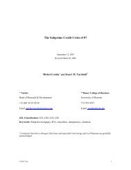
Figure 1: Histograms for the aggregated EC at confidence level of 99 % for the beta model (left) and the
triangular model (right). The posterior mean and the 95 % percent credible interval can be calculated to
37.89 [36.63, 39.24] and 37.90 [36.59, 39.27] for the beta and triangular model, respectively, corresponding
to a relative uncertainty of the aggregated EC of about 7 %.
account. Results for the beta and triangular prior models as well as for the “standard”
approach using one fixed matrix B are given in Table 4.5. The posterior distribution of
the inter-risk-correlation matrix implies also a posterior distribution for the aggregated
EC which can be used to analyse the uncertainty of a bank’s aggregated EC figure and
thus also the diversification benefit due to risk-type dependence. Particularly useful are
graphical methods that depict the posterior density of the aggregated EC at confidence
level κ, denoted by pEC(κ)(·), e.g. histograms (as shown in Figure 1) or “uncertainty” plots
like in Figure 2. The latter illustrates the density pEC(κ)(·) as a function of the confidence
level κ by means of a gray-level intensity plot. Other useful measures of uncertainty
are credible intervals, which are direct probability statements about model parameters or
functions of it given the observed data (see e.g. Berger [4]). We calculated the 95 % percent
15

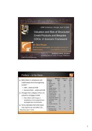
Figure 2: Uncertainty plot for the aggregated EC if the priors for the pair correlations are described by
triangular distributions as in Example 3.3. Lighter (darker) shaded regions of the plot indicate a lower
(higher) posterior density of the aggregated EC.
credible interval for the EC distributions given in Figure 1. In case of the beta priors we
obtain [36.63, 39.24] and for the triangular shaped priors a calculation yields [36.59, 39.27].
Obviously, in our numerical example, one can see from Table 4.5 and Figure 1 that the
impact of differently shaped priors (with equal means and standard deviations, however)
on the aggregated EC can be neglected.
5 Expert judgement and
subjective prior assessment
This Section is devoted to the selection of appropriate prior distributions for the corre-
lation matrix R of the Gaussian copula. In typical risk-aggregation problems data are
scarce and therefore it is worthwhile to study how available subjective information or
prior beliefs about inter-risk correlations can be accounted for in a formal and sound way.
The necessity for expert judgement Clearly, if almost perfect empirical data were
available (e.g. complete, reliable, and representative risk-proxy time series for each risk
type) then it would be acceptable to rely only on statistical correlation estimates to
approximate inter-risk dependence. Unfortunately, in practice it is often extremely difficult
to identify and gather high-quality risk proxies for each risk type making the estimation
16

of inter-risk correlations a tricky exercise.
There are several reasons for these difficulties. First, there is the question regarding
internal versus external data. The general opinion is that risk proxies should be derived
from bank-internal data because it is more related to the companies’s specific business
strategy. However, internal time series may be hard to come by or difficult to re-build
after a merger or a company’s re-organisation, resulting in quite short risk-proxy time
series reducing the statistical significance of correlation estimates. A consequence thereof
is that bank-internal proxies are often amended by external data, at least for some risk
types. Another problem is to find a common frequency that provides a natural scale for
all risk types. Usually, risk proxies for different risk types are measured at unequal time
intervals and therefore further assumptions and approximations have to be used to make
risk proxies comparable. For example, market risk data are available at a daily basis
whereas proxies for business risk are often based on accounting information and therefore
exist only at quarterly or even yearly level, creating a bottleneck for statistical correlation
estimation.
These drawbacks of a purely statistical analysis based on risk proxies show that it is
often necessary to include a new dimension, namely expert judgement. The usage of some
kind of judgemental approaches when assessing inter-risk correlations is very popular in
the banking industry, however, most of the employed approaches lack a sound scientific
basis. For instance, the widely used method of “ex-post adjustments” of the statistical
correlation estimates cannot be properly formalised, thereby nourishing fears and doubts
concerning the final figures.
In contrast to this, a Bayesian approach for risk aggregation such as we are proposing
here allows to treat empirical data on the one hand and expert knowledge on the other as
two distinct sources of information that are eventually amalgamated by means of Bayes
theorem. In this way it is possible to exploit at the maximum extent both information
sets without contamination effects (i.e. experts that are biased (“anchored”) by the data
and, vice versa, data that is manipulated by the expert).
The Bayesian choice for risk aggregation means that the experts’ beliefs about the as-
sociation between different risk types have to be encoded in the pairwise correlation priors
πi(·) for i = 1, . . . , 6, introduced in Section 3.1. This process is referred to as elicitation
of the prior distributions. Elicitation is a difficult task and a number of different compe-
tencies are required to perform it correctly, not only from a statistical point of view but
also on the psychological side. A readable textbook on this intriguing subject is O’Hagan
et al. [19]. Without going into detail, we want to mention that people are typically em-
ploying only a few strategies or heuristics to quantify uncertainty or to make decisions
under uncertainty, see e.g. Tversky & Kahneman [25]. Consequently, the way questions
17

are asked and how answers are interpreted by the facilitator is crucial, in particular, it
is advisable to collect expert judgements stemming from different elicitation approaches
to be able to double check their internal consistency. Therefore, our suggestion here is to
elicit pairwise correlations by asking questions about the following three kind of variables,
which then can be used to compute the related copula parameters.
(1) Kendall’s tau rank correlations between two distinct risk types,
(2) conditional loss probabilities between two distinct risk types,
(3) joint loss probabilities between two distinct risk types.
Since we elicit single pair correlations we do not account for positive semidefiniteness of
the entire correlation matrix. As explained in Section 3.1 this is done within the MCMC
algorithm.
Correlation elicitation using Kendall’s tau Asking experts to quantify an inter-
risk correlation directly is not a trivial task. Direct assessment of a dependence measure
implies deep knowledge of the relative behaviour of each pair of variables or, in our case, of
two risk types. Moreover, direct estimation of a correlation coefficient should be supported
by a thorough explanation of which kind of measure one actually is interested in.
The most common correlation measure used in practice is Pearson’s linear correlation
coefficient. However, it is well-known that this measure is not consistent with Gaussian
copula risk aggregation unless the joint risk-type distribution is multivariate elliptical, see
e.g. Embrechts, McNeil & Straumann [11]. Furthermore, it is by far not clear whether
Pearson’s linear correlation is really the kind of association measure people are thinking
of when being asked about “correlations”. With this respect, our main concern is that the
liner correlation corr(X, Y ) between two risk types X and Y depends not only on their
dependence structure but also on the specific form of the marginal distribution functions
FX and FY . Therefore, experts will only interpret and estimate a linear correlation cor-
rectly if they also account for the specific marginal distribution functions assumed for X
and Y . Another problem is the counter-intuitive fact that for given risk-type marginals
FX and FY the attainable correlations lie, in general, in a subinterval of [−1, 1]. All these
problems have to be clarified before beginning the elicitation experiment since naive, am-
biguous questions about some kind of risk-type “correlation” may lead the expert to give
an answer biased by her cognitive notion of correlation that probably significantly differs
from the Gaussian copula parameter we are actually interested in.
A possible loophole is an alternative concept of association, namely that of Kendall’s
tau rank correlation τ, which is particularly useful when—as in our case—a multivariate
elliptical problem is assumed, cf. for instance Embrechts, Lindskog & McNeil [10], and
18

with an application to risk-type aggregation and elicitation Böcker [5]. The benefit for
expert elicitation is due to a relationship between Kendall’s tau τi and the associated
Gaussian copula parameter ri, which holds true for essentially all elliptical distributions,
namely
ri = sin(π τi/2) , i = 1, . . . , 6 . (5.1)
Recall that τi ∈ [−1, 1], with τi = 1, (τi = −1) for complete positive (negative) depen-
dence, and τi = 0 for independent risk types. Our suggestion is now to ask experts about
their correlation estimates within an interval [−1, 1] where τi = {−1, 0, 1} can be used as
anchors helping experts to calibrate their answers. Finally, the elicited value for τi can be
transformed to the copula parameter ri by means of (5.1).
Correlation elicitation using conditional and joint probabilities The correla-
tion assessment described above requires the expert to think about two random variables
simultaneously, i.e. it is a bivariate elicitation problem. A natural way to lower the com-
plexity of the elicitation procedure is to reduce it to a univariate space. Specifically, it has
been argued in Gokhale & Press [13] or O’Hagan et al. [19] that one-dimensional problems
are more feasible for expert judgement as experts elicit univariate variables with a higher
degree of accuracy.
Correlation elicitation by means of indirect questions about conditional and joint prob-
abilities was already described in Böcker [5] so that hrere we only briefly summarise the
main results. First note that if d risk types are jointly distributed with a Gaussian copula
with correlation matrix (Rij)ij, i, j = 1, . . . , d, any two risk types l and m (m = l) are
coupled by a Gaussian copula with correlation parameter Rlm. Hence it is sufficient to
consider the bivariate estimation problem.
For two risk-type variables X and Y (and the definition that losses are positive) we
can express their joint survival probability as
P (X > x, Y > y) = 1 − P (X ≤ x) − P (Y ≤ y) + P (X ≤ x, Y ≤ y)
= 1 − FX(x) − FY (y) + CR(FX(x), FY (y)) , x, y > 0 , (5.2)
where FX and FY are the marginal distribution functions of X and Y , respectively, and
CR(·, ·) is a bivariate Gaussian copula with unknown parameter R. Similarly, one may
consider conditional loss probabilities of the form
P (X > x|Y > y) =
P (Y > y, X > x)
P (Y > y)
, x, y > 0 , (5.3)
which depend on the copula correlation R via (5.2). Our strategy is now to elicit such joint
and conditional probabilities for different threshold values of x and y. Since we assume
19

0.1 0 0.1 0.2 0.3 0.4 0.5 0.6 0.7 0.8 0.9 1
0.1 0 0.1 0.2 0.3 0.4 0.5 0.6 0.7 0.8 0.9 1
Correlation
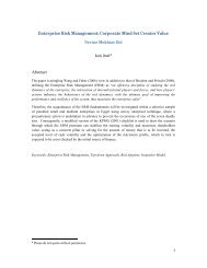
Figure 3: Beta prior and triangular prior obtained by moment matching. It is assumed that the experts’
estimates of some pair correlation are r∗ i = {0.1, 0.2, 0.3, 0.35, 0.4}, yielding r∗ i = 0.27 and var(r∗ 0.0145.
i ) =
that the marginal distribution functions FX and FY are known and already completely pa-
rameterised, one can use relationships (5.2) and (5.3) to determine the copula correlation
R, usually by numerical of graphical methods.
The result of the entire expert elicitation program is that for each pairwise correlation
ri, i = 1, . . . , 6, one obtains a sample r ∗ i := {r ∗ i1, . . . , r ∗ iNi } of Ni expert estimates. The
elicited values r ∗ i may arise from one expert who was confronted with all of the three
approaches suggested above, or may reflect different opinions about risk-type dependence
stemming from several different experts. Now, the experts’ point estimates r ∗ i , i = 1, . . . , 6,
can be used to determine the hyperparameters of the pairwise correlation priors πi(·), i =
1, . . . , 6. For the beta and triangular models these are only two parameters αi and βi for
each pair correlation. Therefore, a viable approach is moment matching because, as shown
in Examples 3.2 and 3.3, we only need to decide about the prior means and variances to
fully determine all πi(·), i = 1, . . . , 6. This approach is illustrated in Figure 3.
20

6 Appendix
6.1 Convergence analysis
As pointed out before, we already know that the algorithm converges theoretically. The
question which must still be answered is if the chain length is long enough. First, we remark
that even if we would took only one iteration in the Metropolis-Hastings algorithm, the
Gibbs sampler would still converge, see Müller [17] and [18]. However our considerations
showed that the Gibbs convergence is faster if we use 1000 iterations of the Metropolis-
Hastings parts.
If we consider now the full chain (R (t) )0≤t≤I Gibbs generated by the algorithm of Section
3.2, we can monitor the convergence by analysing the series s
t=0 det(R(t) ) for
0 ≤ s ≤ IGibbs. This is a standard test procedure for MCMC methods, see e.g. Sec-
tions 7 and 10 of Robert and Casella [21]. The results for our chains were quite fine and
supported the assumption that a burn-in period of 10 percent of the chain is a good
choice.
Second, we applied the Durbin-Watson test to check for autocorrelation in the chain.
If there is not any, the value of the corresponding statistic should be around 2. However, in
order to be able to use this test in our high-dimensional situation we applied the following
trick: If two random variables A and B are independent and if the function f is defined
and measurable on the image of A and B, then f(A) and f(B) are also independent.
Choosing f(·) = det(·) we then investigated the autocorrelation of the transformed chain
det(R (t) )0≤t≤I Gibbs .
For the triangular model the Durbin-Watson statistic was about 1.84, which is good
enough to assume that there is no autocorrelation in the chain. When considering the
chain of the beta model, the analysis yielded a Durbin-Watson statistic of 1.43, indicating
considerable autocorrelation of the chain. Therefore we took only every third value of
the Markov chain to reduce the observed autocorrelation (resulting in a Durbin-Watson
statistic of about 1.94).
6.2 Figures of the posterior distributions
Figures 4 and 5 we illustrate the marginal posterior distributions of all risk-type correla-
tions ri, i = 1, . . . , 6 by means of histograms. Additionally, for each pair correlation the
beta or triangular prior distribution is depicted as a solid line.
21

0.1 0.2 0.3 0.4 0.5 0.6 0.7 0.8 0.9 1
0 0.1 0.2 0.3 0.4 0.5 0.6 0.7 0.8 0.9
Correlation MRCR
0.1 0.2 0.3 0.4 0.5 0.6 0.7 0.8 0.9 1
0 0.1 0.2 0.3 0.4 0.5 0.6 0.7 0.8 0.9
Correlation MRBR
0.1 0.2 0.3 0.4 0.5 0.6 0.7 0.8 0.9 1
0 0.1 0.2 0.3 0.4 0.5 0.6 0.7 0.8 0.9
Correlation CRBR
0.1 0.2 0.3 0.4 0.5 0.6 0.7 0.8 0.9 1
0 0.1 0.2 0.3 0.4 0.5 0.6 0.7 0.8 0.9
Correlation MROR
0.1 0.2 0.3 0.4 0.5 0.6 0.7 0.8 0.9 1
0 0.1 0.2 0.3 0.4 0.5 0.6 0.7 0.8 0.9
Correlation CROR
0.1 0.2 0.3 0.4 0.5 0.6 0.7 0.8 0.9 1
0 0.1 0.2 0.3 0.4 0.5 0.6 0.7 0.8 0.9
Correlation ORBR
Figure 4: Histograms of the simulated marginal posterior distributions for the six pair correlations ri, i =
1, . . . , 6, when the pairwise priors are beta distributed according to Example 3.2. The solid graphs are
the pairwise prior distributions and the dotted lines indicate the empirical correlations of (4.1).
22

0.1 0.2 0.3 0.4 0.5 0.6 0.7 0.8 0.9 1
0 0.1 0.2 0.3 0.4 0.5 0.6 0.7 0.8 0.9
Correlation MRCR
0.1 0.2 0.3 0.4 0.5 0.6 0.7 0.8 0.9 1
0 0.1 0.2 0.3 0.4 0.5 0.6 0.7 0.8 0.9
Correlation MRBR
0.1 0.2 0.3 0.4 0.5 0.6 0.7 0.8 0.9 1
0 0.1 0.2 0.3 0.4 0.5 0.6 0.7 0.8 0.9
Correlation CRBR
0.1 0.2 0.3 0.4 0.5 0.6 0.7 0.8 0.9 1
0 0.1 0.2 0.3 0.4 0.5 0.6 0.7 0.8 0.9
Correlation MROR
0.1 0.2 0.3 0.4 0.5 0.6 0.7 0.8 0.9 1
0 0.1 0.2 0.3 0.4 0.5 0.6 0.7 0.8 0.9
Correlation CROR
0.1 0.2 0.3 0.4 0.5 0.6 0.7 0.8 0.9 1
0 0.1 0.2 0.3 0.4 0.5 0.6 0.7 0.8 0.9
Correlation ORBR
Figure 5: Histograms of the simulated marginal posterior distributions for the six pair correlations ri, i =
1, . . . , 6, when the pairwise priors are triangular distributed according to Example 3.3. The solid graphs
are the pairwise prior distributions and the dotted lines indicate the empirical correlations of (4.1).
23

References
[1] J. Barnard, R. McCulloch, X.-L. Meng, Modeling covariance matrices in terms of
standard deviations and correlations, with application to shrinkage. Statistica Sinica
10, 1281-1311, (2000)
[2] Basel Committee on Banking Supervision (BCBS), Findings on the interaction of
market and credit risk, Working Paper 16, BIS. (2009)
[3] Basel Committee on Banking Supervision (BCBS), Range of practices and issues in
economic capital frameworks, BIS. (2009)
[4] J. O. Berger, Statistical Decision Theory and Bayesian Analysis, 2nd ed., Springer-
Verlag, New York, (1985)
[5] K. Böcker, Aggregation by Risk Type and Inter Risk Correlation, In: Pillar II in the
New Basel Accord – The Challenge of Economic Capital, Ed. A. Resti, Risk Books,
London, 313-344, (2008)
[6] M. Brockmann, M. Kalkbrener, On the Aggregation of Risk, Working Paper, Deutsche
Bank, (2008)
[7] U. Cherubini, E. Luciano, W. Vecchiato, Copula methods in finance, John Wiley &
Sons, Chichester, West Sussex, (2004)
[8] Committee of European Banking Supervisors (CEBS): Consultation paper on tech-
nical aspects of diversification under Pillar 2 (CP20), Consultation Paper, (2008)
[9] X. K. Dimakos, K. Aas, Integrated Risk Modelling, Statistical Modelling 4, 265-277,
(2004)
[10] P. Embrechts, F. Lindskog, A. McNeil, Modelling Dependence with Copulas and Ap-
plications to Risk Management, In: Handbook of Heavy Tailed Distributions in Fi-
nance, Ed. S. Rachev, Elsevier, 329-384, (2001)
[11] P. Embrechts, A. McNeil, D. Straumann, Correlation and dependence in risk man-
agement: properties and pitfalls, In: Risk Management: Value at Risk and Beyond,
Ed. M.A.H. Dempster, Cambridge University Press, Cambridge, 176-223, (2002)
[12] W. R. Gilks, S. Richardson, D. J. Spiegelhalter (Eds.), Markov Chain Monte Carlo
in Practice, Chapman & Hall, London (1996)
24

[13] D. V. Gokhale, S. James Press, Assessment of a Prior Distribution for the Correla-
tion Coefficient in a Bivariate Normal Distribution, Journal of the Royal Statistical
Society A, 145(2), 237-249, (1982)
[14] P. Hartmann, M. Pritsker, T. Schuermann (Eds.), Interaction of market and credit
risk, Special Issue of the Journal of Banking and Finance, forthcoming (2009)
[15] The Institute of the Chief Risk Officers/Chief Risk Officer Forum, Insights from
the joint IFRI/CRO Forum survey on Economic Capital practice and applications,
(2007)
[16] G. Kretzschmar, A.J. McNeil, A. Kirchner, Integrated models of capital adequacy
Why banks are undercapitalised, Technical Report, (2009)
Available at http://www.ma.hw.ac.uk/ mcneil/ftp/WhyBanksUndercapitalised.pdf
[17] P. Müller, A generic approach to posterior integration and Gibbs sampling, Technical
Report, Purdue Univ., West Lafayette, Indiana, (1991)
[18] P. Müller, Alternatives to the Gibbs sampling scheme, Technicl Report, Institute of
Statistics and Decision Sciences, Duke Univ., (1993)
[19] A. O’Hagan et al., Uncertain Judgements: Eliciting Experts’ Probabilities, John Wi-
ley & Sons, Chichester, West Sussex, (2006)
[20] S. J. Press, Applied multivariate analysis: using Bayesian and frequentist methods of
inference, 2nd ed., Dover Publications, Mineola, New York, (2005)
[21] C. P. Robert, G. Casella, Monte Carlo Statistical Methods, 2nd ed., Springer, New
York, (2004)
[22] G. Roberts, Markov chain concepts related to sampling algorithms, In: Markov Chain
Monte Carlo in Practice, Ed.: W. R. Gilks, S. Richardson, D. J. Spiegelhalter, Chap-
man & Hall, London, 45-57, (1996)
[23] J. V. Rosenberg, T. Schuermann, A General Approach to Integrated Risk Manage-
ment with Skewed, Fat-Tailed Risk, Working Paper, Federal Reserve Bank of New
York Staff Reports, no. 185, (May 2004)
[24] F. Saita, Principles of Risk Aggregation, In: Pillar II in the New Basel Accord – The
Challenge of Economic Capital, Ed. A. Resti, Risk Books, London, 297-311, (2008)
[25] A. Tversky, D. Kahneman, Judgment under Uncertainty: Heuristics and Biases, Sci-
ence, (185), 1124-1131, (1974)
25

[26] L. Ward, D. Lee, Practical application of risk-adjusted return on capital framework,
Dynamic Financial Analysis Discussion Paper, CAS Forum, (2002)
26