Bayesian Risk Aggregation: Correlation ... - ERM Symposium

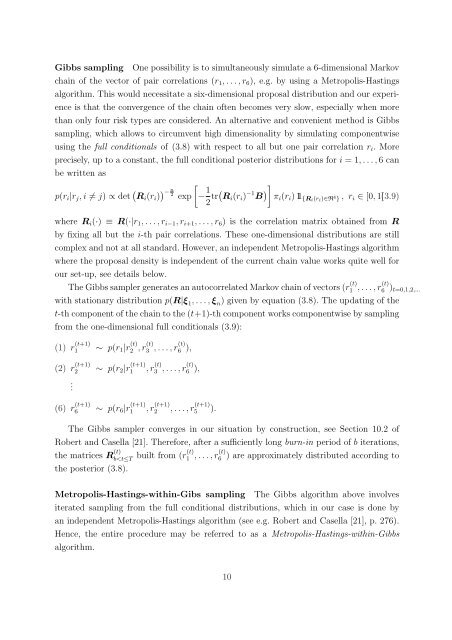
Gibbs sampling One possibility is to simultaneously simulate a 6-dimensional Markov
chain of the vector of pair correlations (r1, . . . , r6), e.g. by using a Metropolis-Hastings
algorithm. This would necessitate a six-dimensional proposal distribution and our experi-
ence is that the convergence of the chain often becomes very slow, especially when more
than only four risk types are considered. An alternative and convenient method is Gibbs
sampling, which allows to circumvent high dimensionality by simulating componentwise
using the full conditionals of (3.8) with respect to all but one pair correlation ri. More
precisely, up to a constant, the full conditional posterior distributions for i = 1, . . . , 6 can
be written as
p(ri|rj, i = j) ∝ det Ri(ri) − n
2 exp − 1
2 trRi(ri) −1 B
πi(ri) 1 {Ri(ri)∈R4 } , ri ∈ [0, 1](3.9)
where Ri(·) ≡ R(·|r1, . . . , ri−1, ri+1, . . . , r6) is the correlation matrix obtained from R
by fixing all but the i-th pair correlations. These one-dimensional distributions are still
complex and not at all standard. However, an independent Metropolis-Hastings algorithm
where the proposal density is independent of the current chain value works quite well for
our set-up, see details below.
The Gibbs sampler generates an autocorrelated Markov chain of vectors (r (t)
1 , . . . , r (t)
6 )t=0,1,2,...
with stationary distribution p(R|ξ 1, . . . , ξ n) given by equation (3.8). The updating of the
t-th component of the chain to the (t+1)-th component works componentwise by sampling
from the one-dimensional full conditionals (3.9):
(1) r (t+1)
1
(2) r (t+1)
2
.
(6) r (t+1)
6
∼ p(r1|r (t)
2 , r (t)
3 , . . . , r (t)
6 ),
∼ p(r2|r (t+1)
1 , r (t)
3 , . . . , r (t)
6 ),
∼ p(r6|r (t+1)
1
, r (t+1)
2
, . . . , r (t+1)
5 ).
The Gibbs sampler converges in our situation by construction, see Section 10.2 of
Robert and Casella [21]. Therefore, after a sufficiently long burn-in period of b iterations,
the matrices R (t)
b