A Calculator for Pareto Points

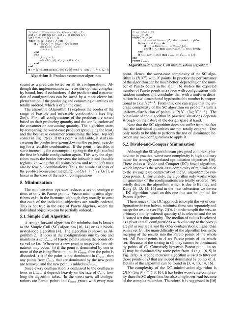
ProducerConsumer(CP , QP , CC , QC, f)
Sort CC on attribute QC, sort CP on attribute QP ;
Let i = 0, j = |CP | − 1;
while i < |CC| and j ≥ 0 do
if CC [i, QC ] f(CP [j, QP ]) then
add CC [i] · CP [j];
i = i + 1;
end
else j = j − 1;
add all CC[k] · CP [j] with k < i;
end
end
if i = |CC| then add all CC[k]·CP [l] with l < j and 0 ≤ k < |CC|;
Algorithm 1: Producer-consumer algorithm
straint as a predicate tested on all its configurations. Although
this implementation achieves the optimal complexity
bound, lots of evaluations of the predicate and construction
of configurations can be saved by a more clever implementation
if the producing and consuming quantities are
totally ordered, which is often the case.
The algorithm (Algorithm 1) explores the border of the
range of feasible and infeasible combinations (see Fig.
2(e)). First, all configurations of the producer are sorted
based on their producing quantity and the configurations of
the consumer on consuming quantity. The algorithm starts
by comparing the worst-case producer (producing the least)
and the best-case consumer (consuming the least, top-left
corner in Fig. 2(e)). If this point is infeasible, it starts increasing
the production (going down in the picture), searching
for a feasible combination. If the point is feasible, it
starts increasing the consumption (going to the right) to find
the first infeasible configuration again. This way the algorithm
traces the border between the infeasible and feasible
regions, knowing that all points below and to the left must
also be feasible combinations. Thus, the number of tests of
the producer-consumer matching, c2(Q2) f(c1(Q1)), is
linear in the sizes of the sets of configurations.
5. Minimisation
The minimisation operator reduces a set of configurations
to only its Pareto points. Vector minimisation algorithms
exist in the literature, although they usually assume
that each of the individual objectives are totally ordered.
This is not true in the case of Pareto Algebra, where the
individual objectives can be partially ordered.
5.1. Simple Cull Algorithm
A straightforward algorithm for minimisation is known
as the Simple Cull (SC) algorithm [16, 14] or as a blocknested-loop
algorithm [4]. The algorithm is shown as Algorithm
2. It looks at the configurations one by one and
maintains a set Cmin of Pareto points among the points observed
so far. Whenever a new point is inspected, two situations
may occur. (i) if the point is dominated by one or
more of the existing Pareto points in Cmin, then the point is
discarded. (ii) if the point is not dominated in Cmin, then
any points from Cmin that are dominated by the new point
are removed and the new point is added to Cmin.
Since every configuration is compared to the configurations
in Cmin, it depends heavily on the size of Cmin how
long the algorithm takes. In the worst case, all configurations
are Pareto points and Cmin grows with every new
SimpleCull(C)
Cmin := ∅;
while C = ∅ do
c := RemoveElement(C); dominated := false;
foreach d ∈ Cmin do
if c d then Cmin := Cmin\{d};
else if d c then dominated := true; break;
end
if not dominated then Cmin := Cmin ∪ {c};
end
return Cmin;
Algorithm 2: Simple Cull minimisation algorithm
point. Hence, the worst-case complexity of the SC algorithm
is O(N 2 ) with N points. In practice the performance
of the algorithm can be much better, depending on the number
of Pareto points in the set. [16] studies the expected
number of Pareto points in a space with configurations with
random numbers and concludes that with a uniform distribution
in a d-dimensional hypercube this number is proportional
to (log N) d−1 . From this, one can argue that the average
complexity of the SC algorithm on problems with a
uniform distribution of points is O(N · (log N) d−1 ). The
behaviour of the algorithm in practical situations depends
strongly on the nature of the design space at hand.
Note that the SC algorithm does not suffer from the fact
that the individual quantities are not totally ordered. One
only needs to be able to perform the test of dominance between
any two configurations to apply it.
5.2. Divide-and-Conquer Minimisation
Although the SC algorithm can give good complexity behaviour
in practice, worst-case complexity is high and may
occur for strongly correlated optimisation objectives [16].
There exists a Divide-and-Conquer (DC) based algorithm,
which improves the worst-case complexity of minimisation
to the average case complexity of the SC algorithm for random
points. Unfortunately, the algorithm only works when
all quantities of the configurations are totally ordered. We
briefly discuss the algorithm, which is due to Bentley and
Kung [3, 13, 14, 16] and in the next subsection we devise
a DC algorithm based on this one that can be applied for
Pareto Algebra.
The essence of the DC approach is to split the set of configurations
in two halves, minimise these sets separately and
merge the results (see Fig. 2(f)). In order to split the sets, an
arbitrary (totally ordered) quantity Q is selected and the set
is sorted wrt that quantity. The median of values is selected
as a pivot and all configurations with values up to the pivot p
are put in one set A and the other configurations, higher than
p, in a set B. The main difficulty of the algorithm lies in the
merging of the results into the Pareto points of the whole
set. All Pareto points in A are Pareto points of the whole
set. Because of the sorting in Q, they cannot be dominated
by points of B. Conversely however, Pareto points in set
B may be dominated by some point from A (e.g., (6,.5) in
Fig. 2(f)). A second recursive algorithm is used to filter out
those points of B that are indeed dominated by points of A.
Details of the algorithm can be found in [3, 4, 13, 14, 16].
The complexity of the DC minimisation algorithm is
O(N ·(log N) d−1 )[3, 16]. It has better worst-case complexity
than the SC algorithm, but also a high overhead because
of the complex recursion. Therefore, it is suggested in [16]