MNEMEE - Electronic Systems - Technische Universiteit Eindhoven

Information Societies Technology (IST) Program
MNEMEE
Memory management technology for adaptive and efficient design of
embedded systems
Contract No IST-216224
Deliverable D1.2
Scenario identification, analysis of static and dynamic data
accesses and storage requirements in relevant benchmarks
Editor: S. Stuijk (TUE)
Co-author / Acknowledgement: Arindam Mallik (IMEC) / Rogier Baert (IMEC) /
Christos Baloukas (ICCS)
Status - Version: Final V1.0
Date: 20/12/2008
Confidentiality Level: Public
ID number: d1-2_tue_v1-0
© Copyright by the MNEMEE Consortium
The MNEMEE Consortium consists of:
Interuniversity Microelectronics Centre (IMEC vzw) Prime Contractor Belgium
Institute of Communication and Computer Systems
(ICCS)
Contractor Greece
Technische Universiteit Eindhoven (TUE) Contractor Netherlands
Informatik Centrum Dortmund e.V. (ICD) Contractor Germany
INTRACOM S.A.Telecom Solutions (ICOM) Contractor Greece
THALES Communications S.A. (TCF) Contractor France

Table of Contents
1. DISCLAIMER ................................................................................................................................6
2. ACKNOWLEDGEMENTS ...........................................................................................................6
3. DOCUMENT REVISION HISTORY ..........................................................................................6
4. PREFACE .......................................................................................................................................7
5. ABSTRACT ....................................................................................................................................8
6. INTRODUCTION ..........................................................................................................................9
7. SCENARIO IDENTIFICATION AND CHARACTERIZATION BASED ON DATAFLOW
GRAPHS ...............................................................................................................................................12
7.1. OVERVIEW ..............................................................................................................................12
7.2. EXISTING SCENARIO IDENTIFICATION AND CHARACTERIZATION TECHNIQUES .....................13
7.2.1. Single-processor scenario identification and exploitation .............................................13
7.2.2. Application characterization using SDF graphs ............................................................14
7.2.3. SDF graph-based multi-processor design-flow .............................................................16
7.3. FSM-BASED SADF .................................................................................................................19
7.4. MULTI-PROCESSOR SCENARIO IDENTIFICATION AND EXPLOITATION ....................................21
7.4.1. Overview.........................................................................................................................21
7.4.2. Source code annotation and application profiling .........................................................23
7.4.3. Scenario cost-space construction and scenario parameter selection ............................24
7.4.4. Scenario formation .........................................................................................................25
7.5. APPLICATION CHARACTERIZATION USING FSM-BASED SADF GRAPHS ................................26
7.6. FSM-BASED SADF-BASED MULTI-PROCESSOR DESIGN-FLOW ..............................................27
7.7. CONCLUSIONS ........................................................................................................................28
8. STATICALLY ALLOCATED DATA STORAGE AND DATA ACCESS BEHAVIOUR
ANALYSIS............................................................................................................................................29
8.1. OVERVIEW ..............................................................................................................................29
8.2. INTRODUCTION TO STATIC DATA OPTIMIZATION IN MEMORY ................................................29
8.3. APPLICATION DESCRIPTION ....................................................................................................32
8.3.1. Introduction to block-based coding ................................................................................32
8.3.2. A Basic Video Coding Scheme .......................................................................................33
8.3.3. Video Coding Standards .................................................................................................34
8.3.4. MPEG-4 part 2 Video Coding Scheme ...........................................................................35
8.4. STATIC DATA CHARACTERISTICS OF THE SCENARIO APPLICATION ........................................35
8.4.1. CleanC specifications overview .....................................................................................36
8.4.2. Atomium Tool Overview .................................................................................................36
8.4.3. Profiling steps ................................................................................................................39
8.4.4. Profiling results for selected functions ...........................................................................40
8.5. DATA-REUSE ANALYSIS ..........................................................................................................42
8.5.1. Introduction ....................................................................................................................42
8.5.2. Identifying data re-use ...................................................................................................44
8.5.3. Exploiting data re-use ....................................................................................................51
8.5.4. Results and conclusion ...................................................................................................55
9. DYNAMICALLY ALLOCATED DATA STORAGE AND DATA ACCESS BEHAVIOUR
ANALYSIS............................................................................................................................................57
9.1. OVERVIEW ..............................................................................................................................57
9.2. INTRODUCTION .......................................................................................................................57
9.3. MOTIVATING DYNAMIC DATA ACCESS OPTIMIZATION ...........................................................58
9.4. MOTIVATING DYNAMIC DATA STORAGE OPTIMIZATION ........................................................60
9.4.1. Shortcomings of static solutions .....................................................................................61
Public Page 2 of 87

9.5. METRICS AND COST FACTORS FOR DYNAMIC DATA ACCESS AND STORAGE OPTIMIZATION ..62
9.5.1. Memory fragmentation (mostly DMM related) ..............................................................62
9.5.2. Memory footprint ............................................................................................................64
9.5.3. Memory accesses ............................................................................................................64
9.5.4. Performance ...................................................................................................................64
9.5.5. Energy consumption .......................................................................................................65
9.6. PRE-MNEMEE DYNAMIC DATA ACCESS AND STORAGE OPTIMIZATION TECHNIQUES ..........65
9.6.1. Dynamic data access optimization .................................................................................65
9.6.2. Dynamic storage optimization .......................................................................................66
9.7. MNEMEE EXTENSIONS TO CURRENT APPROACHES ..............................................................67
9.7.1. Dynamic data access optimization .................................................................................67
9.7.2. Dynamic storage optimization .......................................................................................69
9.8. APPLICATION DESCRIPTION ....................................................................................................70
9.9. LOGGING DYNAMIC DATA ......................................................................................................70
9.9.1. Analysis ..........................................................................................................................72
9.10. CASE STUDY DYNAMIC DATA ANALYSIS ............................................................................73
10. CONCLUSIONS.......................................................................................................................79
11. REFERENCES .........................................................................................................................80
12. GLOSSARY ..............................................................................................................................87
Public Page 3 of 87

List of Tables
Table 1 – Worst-case resource requirements for an H.263 encoder running on an ARM7. ..................16
Table 2 - Platform summary...................................................................................................................55
Table 3 - Comparison of different profiling approaches. .......................................................................71
Table 4 - Profiling information stored by our tools. ...............................................................................73
Table 5 - Memory blocks requested by the application. ........................................................................77
List of Figures
Figure 1 – An interactive 3D game with streaming video based mode [25]. ...........................................9
Figure 2 – Preliminary MNEMEE source-to-source optimizations design flow. ..................................11
Figure 3 – System scenario methodology overview [29]. ......................................................................14
Figure 4 – SDFG of an H.263 encoder. ..................................................................................................14
Figure 5 - SDFG-based MP-SoC design flow [44]. ...............................................................................17
Figure 6 – H.263 encoder mapped onto MP-SoC platform. ..................................................................19
Figure 7 – FSM-based SADF graph of an H.263 decoder. ....................................................................20
Figure 8 – Scenario identification technique. .........................................................................................22
Figure 9 – Extraction of FSM-based SADF from scenario identification technique. ............................26
Figure 10 – Scenario-aware MP-SoC design flow. ................................................................................27
Figure 11 - Power Analysis of a MP-SoC system. .................................................................................30
Figure 12 - Memory hierarchy in embedded systems. ...........................................................................30
Figure 13 - Area and Performance benefits of SPM over cache for embedded benchmarks [15]. ........31
Figure 14 - 4:2:0 macroblock structure. .................................................................................................33
Figure 15 - Video encoder block diagram [18]. .....................................................................................34
Figure 16 - MPEG-4 part 2 SP encoder scheme. ...................................................................................35
Figure 17 - Profiling Steps for Analysis. ................................................................................................39
Figure 18 - Execution time usage by functions (micro seconds). ..........................................................40
Figure 19 - Array size and accesses for selected functionalities. ...........................................................41
Figure 20 - Exploiting the memory hierarchy. .......................................................................................43
Figure 21 - Work flow overview. ...........................................................................................................44
Figure 22 - Data re-use at different loop-levels. ....................................................................................45
Figure 23 - Example re-use graph. .........................................................................................................46
Figure 24 - (Pruned) re-use graph of the motion-vector array. ..............................................................47
Figure 25 - (Pruned) re-use graph of the reconstructed Y-frame demonstrating the results of the XOR
re-use identification algorithm. .......................................................................................................49
Figure 26 - (Pruned) re-use graph of the reconstructed Y-frame for the MPEG-4 motion-estimation
function demonstrating loop-carried copy candidates. ...................................................................50
Figure 27 - Assignment of copies (cf. Figure 23) to memory layers. ....................................................53
Figure 28 - Possible (partial) selection of copies of the reconstructed Y-frame. ...................................54
Figure 29 - Example of pre-fetching. .....................................................................................................54
Figure 30 - A singly linked list (SLL) ....................................................................................................59
Figure 31 - A doubly linked list (DLL) ..................................................................................................59
Figure 32 - A singly linked list with a roving pointer storing the last accessed element. ......................60
Figure 33 - Static memory management solutions fit for static data storage needs and dynamic
memory management solutions fit for dynamic data storage needs. ..............................................61
Figure 34 - Internal (A) and external (B) memory fragmentation..........................................................63
Figure 35 - Software metadata required for behavioural analysis of DDTs. ..........................................68
Figure 36 - Methodological Flow for Profiling Dynamic Applications. ................................................71
Figure 37 - Flow of profiling and analysis tools. ...................................................................................72
Figure 38 - Total data accesses for each DDT. ......................................................................................73
Figure 39 - Maximum Instances for each DDT. ....................................................................................74
Figure 40 - Maximum number of objects hosted in each DDT. .............................................................75
Figure 41 - Iterator access versus operator[] access to elements in a DDT. ..........................................75
Figure 42: Sequential/Random access pattern for each DDT ................................................................76
Figure 43 - Utilization of the allocated memory space by the DDT. .....................................................77
Public Page 4 of 87

Public Page 5 of 87

1. Disclaimer
The information in this document is provided as is and no guarantee or warranty is given that the
information is fit for any particular purpose. The user thereof uses the information at its sole risk and
liability.
2. Acknowledgements
The editor acknowledges contributions by Twan Basten (TUE), AmirHossein Ghamarian (TUE), Marc
Geilen (TUE), Christos Baloukas (ICCS), Arindam Mallik (IMEC) and Rogier Baert (IMEC). The
editor also thanks Bart Mesman (TUE) for his comments on this document.
3. Document revision history
Date Version Editor/Contributor Comments
08/05/2008 V0.0 S. Stuijk (TUE) First draft.
13/09/2008 V0.1 S. Stuijk (TUE) Second draft.
10/11/2008 V0.2 S. Stuijk (TUE) Third draft. Integration of
ICCS, IMEC and TUE
contributions.
19/11/2008 V0.3 S. Stuijk (TUE) Final draft.
20/12/2008 V1.0 S. Stuijk (TUE) Final editing. Final Release
Public Page 6 of 87

4. Preface
The main objectives of the MNEMEE project are:
• provide a novel solution for mapping applications cost-efficiently to the memory hierarchy of
any MP-SoC platform without significant optimization of the initial source code.
• Introducing an innovative supplementary source-to-source optimization design layer for data
management between the state-of-the-art optimizations at the application functionality and the
compiler design layer.
• The efficient data access and memory storage of both dynamically and statically allocated data
and their assignment on the memory hierarchy.
• Use and dissemination of the results.
The expected results of the project are:
• 50% reduction in design time
• 30% reduction in memory footprint and bandwidth requirements
• 50% improved energy and power efficiency
The technological challenges of the project are:
• Provide a framework for source-to-source optimization methodologies, which targets both
statically and dynamically allocated data.
• Introduce a novel source-to-source optimization design layer.
• Analyze the embedded software applications and highlight the source-to-source optimization
opportunities.
• Develop a set of prototype tools.
• Provide data memory-hierarchy aware assignment and scheduling methodologies.
The MNEMEE project has started its activities in January 2008 and is planned to be completed by the
end of December 2010. It is led by Mr. Stylianos Mamagkakis and Mr. Tom Ashby of IMEC. The
Project Coordinator is Mr Peter Lemmens. Five contractors (INTRACOM, Thales, ICD, ICCS and
TUE) participate in the project. The total budget is 2.950 k€.
Public Page 7 of 87

5. Abstract
Embedded software applications use statically and dynamically allocated data objects for which
storage space must be allocated. This allocation should take the access pattern to these data objects
into account in order to minimize the required storage space. This deliverable presents several
techniques to analyze the access behaviour to statically and dynamically allocated data objects. The
aim of these analysis techniques is to identify the different scenarios of data usage and to highlight
optimization opportunities for WP2 and WP3. The deliverable also presents a strategy to model the
application with the identified scenarios in a dataflow graph. This dataflow model can be used to map
an application onto a multi-processor platform while providing timing guarantees and minimizing the
resource usage of the application within each scenario.
Public Page 8 of 87

6. Introduction
Multimedia applications constitute a huge application space for embedded systems. They underlie
many common entertainment devices, for example, cell phones, digital set-top boxes and digital
cameras. Most of these devices deal with the processing of audio and video streams. This processing is
done by applications that perform functions like object recognition, object detection and image
enhancement on the streams. Typically, these streams are compressed before they are transmitted from
the place where they are recorded (sender) to the place where they are played-back (receiver).
Applications that compress and decompress audio and video streams are therefore among the most
dominant streaming multimedia applications [51]. The compression of an audio or video stream is
performed by an encoder. This encoder tries to pack the relevant data in the stream into as few bits as
possible. The amount of bits that need to be transmitted per second between the sender and receiver is
called the bit-rate. To reduce the bit-rate, audio and video encoders usually use a lossy encoding
scheme. In such an encoding scheme, the encoder removes those details from the stream that have the
smallest impact on the perceived quality of the stream by the user. Typically, encoders allow a tradeoff
between the perceived quality and the bit-rate of a stream. The receiver of the stream must use a
decoder to reconstruct the received audio or video stream. After decoding, the stream can be output to
the user, or additional processing can be performed on it to improve its quality (e.g., noise filtering), or
information can be extracted from it (e.g., object detection). There exist a number of different audio
and video compression standards that are used in many embedded multimedia devices. Popular video
coding standards are H.263 [36] (e.g., used for video conferencing) and MPEG-2 [34] (e.g., used for
DVD) and their successors H.264 and MPEG-4 [35][37]. Audio streams are often compressed using
the MPEG-1 Layer 3 (MP3) standard [32] or the Ogg Vorbis standard [38].
Figure 1 – An interactive 3D game with streaming video based mode [25].
Public Page 9 of 87

With modern applications, the streams and their encodings can be very dynamic. Smart compression,
encoding and scalability features make these streams less regular then they used to be. Furthermore,
these streams are typically part of a larger application. Other parts of such an application may be
event-driven and interact with the stream components. Consider for example an imaginary game
application shown in Figure 1, which is taken from [25]. This game includes modes of 3-dimensional
game play with streaming video based modes. The rendering pipeline, used in the 3D mode, is a
dynamic streaming application. Characters or objects may enter or leave the scene because of player
interaction, rendering parameters may be adapted to achieve the required frame rates. Overlay graphics
(for instance text or scores) may change. This happens under control of the event-driven game control
logic. At the core of the application, the streaming kernels, a lot of intensive pixel based operations are
required to perform the various texture mapping or video filtering operations. These operations are
performed on a stream of data items. At each point in time, only a small number of data items from the
stream are being processed. The order in which these data items are accessed has typically little
variation. This makes it possible to optimize the memory access behaviour of the streaming kernels to
achieve the required performance while minimising the energy consumption.
Future embedded systems are not only characterized by their increasingly dynamic behaviour due to
different operations modes that may occur at run-time, but also by their dynamism in memory
requirements. Next generation embedded multimedia systems will have intensive data transfer and
storage requirements. Partially these requirements will be static, but partially they will also be
changing at run-time. Therefore, efficient memory management and optimization techniques are
needed to increase system performance and decreased cost in energy consumption and memory
footprint due to the larger memory needs of future applications. It is essential that these memory
management and optimization techniques are supported by design automation tools, because due to the
very complex nature of the source code, it would be impossible to apply them manually in a
reasonable time frame. The automation tools should be able to optimize both statically and
dynamically allocated data, in order to cope with design-time needs and adapt to run-time memory
needs (scalable multimedia input changing at run-time, unpredictable network traffic, etc.) in the most
efficient way. A design flow that realizes these objectives will be developed within MNEMEE. An
overview of the preliminary flow is shown in Figure 2 (The final flow will be presented in D5.3). The
flow takes as input the source code of an application and optimizes the memory behaviour of the
application. The source code of the optimized application is the output of this flow. The first step of
the flow models the source code as a task graph. The output of this step, and all other steps, is a
combination of source code and models that are transferred to the next step. In this step, the task graph
is mapped onto the processing elements that are available in the hardware platform. There will be two
different mapping options available within the MNEMEE flow. The first option, called scenariobased,
takes the dynamic behaviour of the application into account when mapping it onto the platform.
The second option, called memory-aware, considers the memory hierarchy in the platform. After the
mapping, the static and dynamic access behaviour of the application is optimized in the steps labelled
‘parallelization implementation’ and ‘dynamic memory management’. Finally, additional memory
optimizations are applied on a per processor element basis. These optimizations are based on existing
single processor scratchpad optimization techniques [49].
The remainder of this document presents a number of analysis approaches that can be used, within the
context of the design flow, to identify memory access behaviour and dynamic behaviour in
applications. Each of these analysis approaches focuses on different sources of dynamism in
multimedia applications. Section 7 presents techniques to analyze and exploit the dynamically
changing resource requirements of applications. These analysis techniques are part of the scenariobased
approach that can be used within the ‘task graph to processing element mapping’ step of the
design flow. The memory-aware approach that can also be used in this step will be developed within
WP4 and described in D4.2. Section 8 presents techniques to analyze the access behaviour to statically
allocated data objects. This section discusses the step labelled ‘parallelization implementation’ in the
design flow of Figure 2. Section 9 focuses on the access behaviour to dynamically allocated data
objects. This section discusses the details of the step labelled ‘dynamic memory management
optimizations’. Finally, Section 10 concludes this deliverable.
Public Page 10 of 87

Figure 2 – Preliminary MNEMEE source-to-source optimizations design flow.
Public Page 11 of 87

7. Scenario identification and characterization based on dataflow graphs
7.1. Overview
The application domain, as sketched in Chapter 6, is characterized by applications which increasingly
exhibit a dynamic behaviour. Due to this dynamic behaviour, applications have resource requirements
that vary over time. The concept of system scenarios has been introduced [29] to exploit these varying
resource requirements. The idea is to classify the operation modes of an application from a cost
perspective into several system scenarios, where the cost within a scenario is fairly similar [28][29].
At run-time, a set of variables that are used in the program, called scenario parameters, can be
observed. These scenario parameters can be used to determine in which scenario the application
operates. The resource reservations for an application running in a system can then be matched to the
requirements of the scenario that is being executed. This should lead to a resource usage that is on
average lower than the worst-case resource requirements of the application when no scenarios are
distinguished.
A heterogeneous multi-processor System-on-Chip (MP-SoC) is often mentioned as the hardware
platform to be used in domain of streaming multimedia applications. An MP-SoC offers good
potential for computational efficiency (operations per Joule) for many applications. When a
predictable resource arbitration strategy is used for the processors, storage elements and interconnect,
the timing behaviour of all hardware components in the platform can be predicted. To guarantee the
timing behaviour of applications, it is further required that the timing behaviour and resource usage of
these application mapped to an MP-SoC platform can be analyzed and predicted. In this way, it
becomes possible to guarantee that an application can perform its own tasks within strict timing
deadlines, independent of other applications running on the system. In [44], a predictable design flow
is presented that maps an application onto a MP-SoC while providing throughput guarantees. This
design flow requires that the application is modelled as a Synchronous Dataflow (SDF) graph. The
SDF Model-of-Computation fits well with the characteristics of streaming applications, it can capture
many mapping decisions, and it allows design-time analysis of timing and resource usage. However, it
cannot capture the dynamic behaviour of an application as is done with scenarios. The design flow
assumes that the SDF model of the application captures the worst-case behaviour of the application.
This results in a mapping in which the resource requirements of the application are larger than when
scenarios would be taken into account.
Existing scenario identification techniques focus on single-processor systems. Typically, they also
focus on a single cost dimension (e.g. processor usage). Future platforms will be heterogeneous multiprocessor
systems that contain different types of processing elements and a hierarchy of storage
elements. A scenario identification technique should take these different resources into account as
different cost dimensions. Multi-processor platforms inherently contain parallelism that should be
considered in the scenario identification. This chapter introduces a new scenario identification
technique that considers multiple cost dimensions and the parallelism offered by multi-processor
systems. It also presents an extension of the SDF model, called Finite State Machine-based Scenario-
Aware Dataflow (FSM-based SADF), which can model the dynamic behaviour of an application, as
captured in its scenarios. Finally, a predictable design-flow is sketched that maps an application
modelled with a FSM-based SADF onto a MP-SoC platform.
The remainder of this chapter is organized as follows. Section 7.2 discusses existing scenario
identification and exploitation techniques. It also provides an overview of existing application
characterization and mapping techniques that are based on synchronous dataflow graphs. Section 7.3
introduces the FSM-based SADF model, which is an extension of the synchronous dataflow model
that can be used to model scenarios. Existing scenario identification and exploitation techniques focus
on a single cost dimension. Section 7.4 introduces a new scenario identification technique that can
take multiple cost dimensions into account (e.g. processor cycles, memory usage). Section 7.5 explains
how an FSM-based SADF model of an application can be constructed after identifying scenarios using
the technique presented in Section 7.4. Section 7.6 sketches a design-flow that can map an application,
Public Page 12 of 87

modelled with an FSM-based SADF, onto a multi-processor platform while providing timing
guarantees on the application.
7.2. Existing scenario identification and characterization techniques
This section describes the scenario identification and application characterization and mapping
techniques that have been developed prior to MNEMEE. It introduces the main concepts and it
provides references to publications on these topics.
7.2.1. Single-processor scenario identification and exploitation
Applications that are running on embedded multimedia systems are full of dynamism, i.e., their
execution cost (e.g., number of processor cycles, memory usage, energy) are environment dependent
(e.g., input data, processor temperature). When such an application is running on a given system
platform it may encounter different run-time situations. A run-time situation is a piece of system
execution that is treated as an atomic unit. Each run-time situation has an associated cost (e.g., quality,
resource usage). The execution of the system is a sequence of run-time situations. The current run-time
situation is only known at the moment that it occurs. However, a set of so called scenario parameters
(i.e. variables in the application) can be used to predict the next run-time situation. The knowledge that
this run-time situation will occur in the near future can be used to adapt the system settings (e.g.,
processor frequency, mapping) to this run-time situation. The number of distinguishable run-time
situations from a system is exponential in the number of scenario parameters. To avoid that all these
situations must be handled separately at run-time, several run-time situations should be clustered into a
single system scenario. This clustering presents a trade-off between the optimization quality and the
run-time overhead of the scenario exploitation.
A general methodology to identify and exploit scenarios has been described in [29]. Figure 3 gives an
overview of this methodology in which each step has both a design-time and a run-time phase. The
scenario methodology starts with identifying the potential scenario parameters and clustering the runtime
situations into scenarios. During this clustering, a trade-off must be made between the cost of
having more scenarios (e.g., larger code size, more scenario switches) and the cost of grouping runtime
situations in one scenario (e.g., over-dimensioning of the system for certain run-time situations).
The second step of the scenario methodology is to construct a predictor that at run-time observes the
scenario parameters and that uses their observed values to select a scenario at run-time. The selected
scenario is executed at run-time in the exploitation step. At design-time, this exploitation step
performs an optimization on each scenario individually. During run-time it might be required to switch
between different scenarios. During this switching, the system settings of the old scenario are changed
to the settings required for the new scenario (e.g., processor frequency, memory mapping may be
changed). The switching step selects at design-time an algorithm that is used at run-time to decide
whether to switch or not. It also decides on how a switch should be performed whenever a switch is
required. Finally, the calibration step complements all earlier steps. This step gathers at run-time
information about the scenario parameters and the occurrence and switching frequency of run-time
situations. Infrequently, it uses this information to recalibrate the scenario detector, scenario
exploitation and scenario switching mechanism. This calibration mechanism can further exploit runtime
variations in the observed behaviour, in particular when the encountered behaviour deviates from
the average behaviour considered at design time, and it can correct for imperfections in the designtime
analysis.
Public Page 13 of 87

Figure 3 – System scenario methodology overview [29].
In [29], a case study is presented in which the concept of system scenarios is applied to an MP3
decoder. The objective is to discover scenarios that have a different worst-case execution time
(WCET). This difference in WCET can then be exploited by using dynamic voltage-frequency scaling
(DVFS) on the processor that is executing the MP3 decoder. Using a scenario identification tool, a
total of 41 scenario parameters are discovered. Based on these parameters, the tool discovers a total of
17 different scenarios. The experimental results show that the use of these scenarios leads to an energy
reduction of 24% for a mixed set of stereo and mono streams. It is also shown that the obtained energy
improvement represents more then 72% of the maximum theoretically possible improvement. This
case study shows that system scenarios can successfully be used to exploit similarities in the behaviour
of an application to reduce its resource requirements (e.g., energy usage).
7.2.2. Application characterization using SDF graphs
Multimedia applications are typically streaming applications. The class of dataflow Models-of-
Computation (MoCs) fits well with this behaviour. A dataflow program is specified by a directed
graph where the nodes (called actors) represent computations that communicate with each other by
sending ordered streams of data-elements (called tokens) over their edges. The execution of an actor is
called a firing. When an actor fires, it consumes tokens from its input edges, performs a computation
on these tokens and outputs the result as tokens on its output edges. The Synchronous Dataflow (SDF)
MoC has recently become a popular MoC to model streaming applications [44]. Actors in an SDF
graph (SDFG) consume and produce a fixed amount of tokens on each firing. This makes it possible to
analyze the throughput [23] and latency [27][33][43] of these graphs. An example of an SDFG
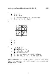
modelling an H.263 encoder is shown in Figure 4.
Figure 4 – SDFG of an H.263 encoder.
In the remainder of this section it is explained how the SDFG shown in Figure 4 can be derived from
the description and source code of the application. First the structure of the SDFG is derived by
Public Page 14 of 87

analyzing the basic operations of the application and the dependencies between these operations. An
H.263 encoder divides a frame in a set of macro blocks (MBs). A macro block captures all image data
for a region of 16 by 16 pixels. The image data inside a MB can be subdivided into 6 blocks of 8 by 8
data elements. Four blocks contain the luminance values of the pixels inside the MB. Two blocks
contain the chrominance values of the pixels inside the MB. A frame with a resolution of 174 by 144
pixels (QCIF) contains 99 MBs. These 99 MBs consist, in total, of 594 blocks. The various operations
that must be performed in a H.263 encoder are modelled as separate actors in the SDFG. The motion
estimation operation is modelled with the Motion Est. actor. The motion compensation and the
variable length encoder operations are modelled with the Motion Comp. and VLC actors. The MB
decoding (MB Dec.) actor models the inverse DCT operation. The DCT and quantization operations
are modelled together in the MB encoding (MB Enc.) actor. The motion estimation, motion
compensation and variable length encoding operations are performed on a complete video frame (i.e.,
99 MBs). The other blocks operations work on a single MB at a time. These different processing
granularities are modelled with the fixed rates in the SDFG of Figure 4. The self-edges on the Motion
Comp. and VLC actors model that part of the data that is used by these actors during a firing must be
stored for a subsequent firing. In other words, these self-edges model the global data that is kept
between executions of the code segments that are modelled with these actors.
The previous paragraph explained how the structure of an SDFG can be derived from the basic
operations that are performed by the application. Some additional information is needed to create an
SDFG that models the application in sufficient detail such that this model can be used in a design
flow. A design flow must allocate resources for the streaming applications that it maps onto a
platform. To do this, the design flow needs information on the resource requirements of the
application being mapped. The application is modelled with an SDFG. The actors in an SDFG
communicate by sending tokens between them. Memory space is needed to store these tokens. The
amount of tokens that must be stored simultaneously can be determined by the design flow. However,
the design flow must know how much memory space is needed for a single token. This is determined
by the number of bytes of the data type that is communicated with the token. This information can
easily be extracted through a static-code analysis. Some information is also needed on the resource
requirements of the actors. These actors represent code segments of the application. To execute a code
segment, processing time is needed as well as memory space to store its internal state. The internal
state contains all variables that are used during the execution of the code segment but that are not
preserved between subsequent executions of the code segment. Global data that is used inside a code
segment is not considered part of the internal state. The SDF MoC requires that global data that is used
by a code segment is modelled explicitly with a self-edge on the actor that models this code segment
(see Figure 4 for an example). This self-edge contains one initial token whose size is equal to the size
of the global data used in the code segment. The maximal size of the internal state is determined by the
worst-case stack size and the maximal amount of memory allocated.
Telenor Research has made a C-based implementation of an H.263 encoder [47]. The techniques
presented in [44] can be used to determine the worst-case execution time and worst-case stack-sizes of
the actors in the H.263 encoder SDF model of Figure 4 when implemented using the implementation
from [47]. These execution times and stack-sizes, assuming that an ARM7 processor is used, are
shown in Table 1. The table shows also the size of the tokens communicated on the edges. The worstcase
stack sizes and worst-case execution times have been obtained through semi-automatic code
analysis of the H.263 encoder. The token sizes are obtained through manual code analysis.
The SDFG shown in Figure 4 combined with the resource requirements shown in Table 1 model an
H.263 decoder as an SDFG. Because worst-case values are used for the execution times and memory
requirements, this model can be used to analyze the worst-case timing behaviour of the application.
This makes the model also suitable for use in a predictable design flow as discussed in the next subsection.
Public Page 15 of 87

Table 1 – Worst-case resource requirements for an H.263 encoder running on an ARM7.
Actor Execution time [cycles] Stack size [bytes]
Motion Est. 382419 316352
Motion Comp. 11356 2796
MB Enc. 8409 2216
MB Dec. 6264 864
VLC 26018 1356
Edge Token size [bytes]
VLC self-edge 1024
Motion Comp. self-edge 38016
Motion Comp. to Motion Est. 38016
Others 384
7.2.3. SDF graph-based multi-processor design-flow
The design of new consumer electronics devices is getting more and more complex as more
functionality is integrated into these devices. To manage the design complexity, a predictable design
flow is needed. The result should be a system that guarantees that an application can perform its own
tasks within strict timing deadlines, independent of other applications running on the system. This
requires that the timing behaviour of the hardware, the software, as well as their interaction can be
predicted. A predictable design-flow that meets these requirements has been presented in [44]. It maps
a time-constrained streaming application, modelled as an SDFG, onto a Network-on-Chip-based MP-
SoC (NoC-based MP-SoC). The objective is to minimize the resource usage (processing, memory,
communication bandwidth) while offering guarantees on the throughput of the application when
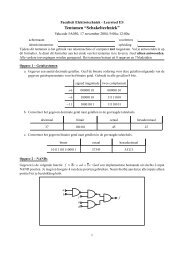
mapped to the system. The design flow presented in [44] is also shown in Figure 5. The design flow
consists of thirteen steps which are divided over four phases. This section introduces the various
phases in the flow. The details of the individual steps and the motivation for the ordering of the steps
in the flow can be found in [44].
The design flow takes as input an application that is modelled with an SDFG with accompanying
throughput constraint. A technique to characterize an application with an SDFG has been discussed in
Section 7.2.2. This SDFG specifies for every actor the required memory space and execution time for
all processors on which this actor can be executed. It also gives the size of the tokens communicated
over the edges. The resources in the NoC-based MP-SoC are described with a platform graph and an
interconnect graph. The result of the design flow is an MP-SoC configuration which specifies a
binding of the actors to the processors and memories, a schedule for the actors on the processors and a
schedule for the token communication over the NoC.
Tokens that are communicated over the edges of an application SDFG must be stored in memory. The
allocation of storage space for these tokens is dealt with in the memory dimensioning phase. This
involves the placement of tokens into memories that are outside the tile that execute the actor that uses
these tokens. Furthermore, storage space must be assigned to the channels of the SDFG. Since the
assignment of the storage space impacts the throughput of the application, an analysis is made of this
trade-off space. Based on this analysis, a distribution of storage space over the channels is selected.
All design decisions that are made in this phase of the design flow are modelled into the SDFG. The
resulting SDFG is called a memory-aware SDFG.
Public Page 16 of 87

Figure 5 - SDFG-based MP-SoC design flow [44].
The next phase of the design flow, called constraint refinement, computed latency and bandwidth
constraints on the channels of the SDFG. These constraints are used to steer the mapping of the SDFG
Public Page 17 of 87

in the tile binding and scheduling phase. This phase binds actors and channels from the resource-aware
SDFG to the resources in the platform graph. When a resource is shared between different actors or
applications, a schedule should be constructed that orders the accesses to the resource. The accesses
from the actors in the resource-aware SDFG to a resource are ordered using a static-order schedule.
TDMA scheduling is used to provide virtualization of the resources to the application.
The third phase of the design flow does not consider the scheduling of the communication on the NoC.
This problem is considered in the NoC routing and scheduling phase of the design flow. The actor
bindings and schedules impose timing-constraints on the communication that must be met when
constructing a communication schedule. These timing constraints are extracted from the bindingaware
SDFG and subsequently a schedule is constructed for the token communication that satisfies
these timing constraints while minimizing the resource usage.
The mapping of the streaming application to the NoC-based MP-SoC may fail at various steps of the
design flow. This may occur due to lack of resources (step 7) or infeasible timing constraints (step 9
and 12). In those situations, the design flow iterates back to the first or third step of the flow and
design decisions made in those steps are revised.
Consider as an example the H.263 encoder shown in Figure 4. This application has been mapped,
using the predictable design flow, onto a multiprocessor platform that consists of two general purpose
processors and three accelerators. These processing elements are interconnected using a Network-on-
Chip. The resulting MP-SoC configuration is shown in Figure 6. The predictable design flow has been
implemented in SDF 3 [45]. It takes this tool 415ms to find a MP-SoC configuration that satisfies the
throughput constraints of the application, while at the same time it tries to minimize the resource usage
of the application.
Public Page 18 of 87

Figure 6 – H.263 encoder mapped onto MP-SoC platform.
7.3. FSM-based SADF
The SDF Model-of-Computation (MoC) is introduced in Section 7.2.2. That section also shows how
an application can be modelled with an SDFG. The SDF model of an application assumes worst-case
rates for the edges and worst-case execution times for the actors. In the situation that an application
contains a lot of dynamism, the use of worst-case values could lead to over-dimensioning of the
system for many run-time situations. Therefore, the concept of system scenarios has been introduced
in [28][29] (see also Section 7.2.1). However, these scenarios cannot be modelled into an SDFG. This
section introduces an extension to the SDF MoC that can be used to model an application together
with its scenarios. This new MoC is called the Finite State Machine-based Scenario-Aware Data-Flow
(FSM-based SADF) MoC.
The FSM-based SADF MoC is a restricted form of the general SADF MoC that has been introduced in
[48]. These restrictions make analysis of the timing behaviour of a model specified in the FSM-based
SADF MoC faster than a model specified in the general SADF MoC. However, analysis result may be
less tight due to the abstractions made in the FSM-based SADF MoC. A formal definition of the FSMbased
SADF MoC and a discussion on the differences between this MoC and the general SADF MoC
can be found in [46]. Here, we focus on an example.
Public Page 19 of 87

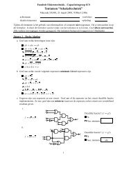
Figure 7 shows the example of an H.263 decoder that is modelled with an FSM-based SADF graph.
The nodes represent the processes of an application. Two types of processes are distinguished. Kernels
model the data processing part of a streaming application, whereas the detector represents the part that
dynamically determines scenarios and controls the behaviour of processes. The Frame Detector (FD)
represents for example that segment of the actual Variable Length Decoder (VLD) code that is
responsible for determining the frame type and the number of macro blocks to decode. All other
processes are kernels. In the FSM-based SADF graph shown in Figure 7, it is assumed that two
different types of frame exists (I or P type). When a frame of type I is found, a total of 99 macro
blocks must always be processed. A frame of type P may require the processing of (up to) 0, 30, 40,
50, 60, 70, 80, or 99 macro blocks. So, in total 9 different scenarios (combinations of frame type and
number of macro blocks to decoder) exist and must be modelled in the graph. These 9 scenarios
capture the varying resource requirements of the application.
Figure 7 – FSM-based SADF graph of an H.263 decoder.
The edges in an FSM-based SADF graph, called channels, denote possible dependencies between
processes. Two types of channels are distinguished. Control channels (dashed edges) originate from
the detector and go to a kernel. Data channels (solid edges) originate from a kernel and go to another
kernel or to the detector. Ordered streams of data items (called tokens) are sent over these channels.
Similar to the SDF MoC, the FSM-based SADF MoC abstracts from the value of tokens that are
communicated via a data channel. However, control channels communicate tokens that are valued.
The value of a token on a control channel indicates the scenario in which the receiving kernel will
operate. This token value is determined externally by the detector. In the example application, the
scenario is determined by the frame type and the number of macro blocks. In reality, this scenario is
determined based on the content of the video stream. However, the FSM-based SADF model abstract
from such content. It uses a (non-deterministic) FSM which determines the possible scenario
occurrences. The states in the FSM determine the scenario in which the kernels will operate. The
Public Page 20 of 87

transitions reflect possible next scenarios given the current scenario that the detector is in. Figure 7
shows part of the FSM for the H.263 decoder. The first scenario that is executed is the scenario in
which a frame of type I is decoded. This frame (scenario) may be followed by another I frame, or a
scenario in which one or more P frames with zero macro blocks are executed followed by an I frame,
or a scenario in which two P frames with 99 macro blocks each are executed followed by an I frame.
7.4. Multi-processor scenario identification and exploitation
Future embedded multimedia systems will use a MP-SoC that contains different types of processing
elements and a hierarchy of storage elements. As explained in Section 7.1, a scenario identification
technique should take these different resources into account as different cost dimensions (e.g.
processor usage, memory usage). This section outlines a scenario identification approach that
considers multiple cost dimensions.
7.4.1. Overview
Streaming multimedia applications are implemented as a main loop, called the loop of interest, which
is executed over and over again, reading, processing and writing out individual stream objects. A
stream object may, for example, be a video frame or an audio sample. Typically, not all stream objects
within a stream are processed in exactly the same way. A video decoder, for example, may distinguish
different inter and intra-coded frames, which must be processed differently. As a result, an application
will have different run-time situations. Each run-time situation has a set of associated costs, like the
number of processors and the amount of memory that is used. As explained in Section 7.2.1, it is
impossible to consider every run-time situation in isolation when designing a system. To solve this
problem, run-time situations must be grouped from a cost perspective into several system scenarios,
where costs within a scenario are fairly similar. So, run-time situations of an application that are
grouped into different scenarios have different costs. These different costs can be exploited at run-time
with the objective to match the resource usage of a system scenario to its requirements. This should
lead to a resource usage that is on average lower than the worst-case resource requirements of the
application when no scenarios are distinguished. Due to the presence of multiple cost dimensions,
there may be multiple “optimal” solutions for mapping a scenario onto a hardware platform. These
solutions provide a trade-off between the different resources (e.g. processors, memories) that are
available in the platform.
The costs that should be taken into account when identifying scenarios depend on the exploitation
options that are available in the hardware platform. On a platform that offers dynamic voltagefrequency
scaling (DVFS) it is interesting to consider the number of processor cycles (execution time)
that is needed to process a run-time situation as a cost of this run-time situation. Typically there is a
timing constraint with the application that specifies bounds on the time that may be spent on
processing a run-time situation (i.e. latency) and on the time between subsequent run-time situations
(i.e. throughput). Given these timing constraints and the number of processor cycles needed to execute
a run-time situation, the optimal DVFS setting can be computed for each scenario. On a platform that
offers a software controlled memory hierarchy it is interesting to consider the number of accesses to
different variables as a cost of this run-time situation. Depending on the amount of accesses to the
variables a different mapping of the variables onto the memory hierarchy can be selected. These
different mappings should reduce the total time needed for memory accesses within each scenario.
Potentially it can also reduce the energy consumption of the platform.
Public Page 21 of 87

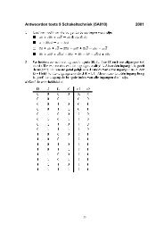
Figure 8 – Scenario identification technique.
In [28], a scenario identification technique is presented that follows the system scenario methodology
as shown in Figure 3. This scenario identification technique focuses on discovering scenarios that can
be exploited on a single-processor system that offers DVFS. The technique uses application profiling
information to analyze the execution behaviour of applications. In an iterative process, variables are
added or removed from the set of potential scenario parameters. When the set of potential scenario
Public Page 22 of 87

parameters is modified, the application profiling is repeated. This process is continued till a set of
scenario parameters is found together with a set of scenarios that minimizes the energy consumption
of the system. A heuristic is used to select the scenario parameters that best characterize the resource
requirements of the application under the various scenarios. This scenario identification technique has
a number of disadvantages. (1) The application must be profiled every time that the set of potential
scenario parameters is modified. This is very time consuming. (2) The selection of scenario parameters
is done using a heuristic that uses knowledge about the specific scenario exploitation mechanism that
is used. Such a heuristic cannot be re-used directly when different (or multiple) cost dimensions are
considered. To alleviate these problems, a new scenario identification technique is presented in Figure
8. The steps of this technique will be explained in detail in the next sections. The main advantages of
this technique are: (1) it allows multiple cost dimensions to be taken into account, (2) no iterative
profiling is required to identify scenario parameters, and (3) the scenario parameter identification
algorithm does not depend on a specific scenario exploitation technique.
7.4.2. Source code annotation and application profiling
The scenario identification technique uses application profiling information to analyze the execution
behaviour of applications. This profiling information should provide information about all aspects that
the user considers relevant when determining scenarios. Depending on the available exploitation
mechanism, the user may for example be interested in the execution time or the memory access pattern
of an application. The former property can be interesting if the platform offers DVFS capabilities or to
obtain tighter (conditional) worst-case bounds. The latter property might be interesting when a
software controlled memory hierarchy is available.
Application profiling requires that the application is executed with one or more input stimuli. During
this execution, the properties of interest (e.g. execution time, memory accesses) can be observed.
However, such a monolithic approach has a large disadvantage when the execution time of the
application must be profiled for a number of different processor types and/or different memory
hierarchies. In that case, a complete functional simulation of the application with all input stimuli must
be performed for each platform. To avoid this problem, the application profiling should be split into
two steps. First, the application should be executed with all input stimuli. During these executions, it is
traced how often a basic block is executed within a run-time situation. As a next step, the actual
properties of interest are computed based on the basic block counts contained in the trace (i.e. profiling
information). By dividing the application profiling into two steps, it is no longer necessary to perform
a complete functional simulation for each processor type 1 . The scenario identification technique uses
the idea to split the profiling into two steps. The application profiling step (step 2 in Figure 8) executes
the application with a set of user-supplied inputs to trace the basic block counts of the application. The
scenario cost-space construction step (step 3) uses these basic block counts to compute the actual
properties of interest that should be considered when identifying scenarios.
Before the application profiling can be performed, the application source code must be annotated with
profiling statements to trace the basic block execution. This source code annotation is performed in the
first step of the scenario identification technique. This step also adds profiling statements to trace the
boundary between subsequent run-time situations. Furthermore, profiling statements must be added to
identify the scenario parameters. Identification of these scenario parameters is one of the main tasks of
the scenario identification technique. It is in general not possible to determine these scenario
parameters through static code analysis. They must be determined in combination with the scenarios.
Therefore, the application profiling information should contain information on when a value is written
to the variables in the application. The scenario identification technique can then in a later stage
determine which parameters must be observed at run-time and which combination of parameter values
describe a scenario. The source code annotation step adds profiling statements to the source code to
trace the write accesses to potential scenario parameters. Since it is not known which parameters will
1
This approach requires that the data-dependent pipelining effects inside the processor are ignored. It is similar
to the approach proposed in [40].
Public Page 23 of 87

e needed to identify the scenarios, the source code annotation step annotates write accesses to all
scalar variables and small arrays.
Once the source code is annotated, it is passed on to the application profiling step. This step compiles
the source code together with a profiling library into an executable simulation model of the
application. Next, the application is simulated with a set of user-supplied input stimuli. During these
simulations profiling information is created that contains the basic block execution counts of the
application and the write accesses to the potential scenario parameters. This information is used in the
scenario cost-space construction step and in the scenario formation step.
The source code profiling that is explained in this section uses very basic execution profiling functions
(i.e. basic block counts and tracing of scalar variable values). Chapter 9 on the other hand describes an
advanced profiling approach that focuses on dynamic data structures. In principle both profiling
approaches can be integrated in one framework. However, given the different functionality
implemented in both profiling approaches, it does not seem useful to combine these profiling functions
into one framework at this point in time.
7.4.3. Scenario cost-space construction and scenario parameter selection
The profiling information contains data on the number of accesses that occur within a run-time
situation to every basic block in the application. The scenario cost-space construction step uses this
information to compute the cost of using a resource (e.g. processor usage, memory usage) in every
run-time situation. For each cost dimension that is considered, a user supplied resource cost function is
used to compute the cost of a basic block execution. The resource cost function takes both the access
count to a basic block and the platform characteristics into account when it computes the cost of the
basic block accesses that occurred in a run-time situation. Using the profiling information, the cost of
executing a complete run-time situation can be computed by adding up the costs of the individual
basic blocks that are executed in this run-time situation. When this procedure is repeated for all
considered cost dimensions and all run-time situations contained in the profiling information, a cost
matrix C is obtained. This matrix C is an m x n matrix were each of the m rows gives the values of the
various costs of the application. The n columns correspond to the processing of one run-time situation.
The value of the run-time parameters that correspond to the processing of each run-time situation can
be captured in a parameter matrix P. This matrix P is a p x n matrix were each of the p rows gives the
values of the run-time parameters of the application. The linear relation between the cost and run-time
parameters can be captured in a model (i.e. a matrix M), with C = M · P. The matrices C, M and P
model the cost-space of the application.
The number of run-time parameters can potentially be large since the source code annotation step has
selected all scalar variables and small arrays. The scenario parameter selection step should identify a
subset of the run-time parameters that can still accurately predict the cost of each run-time situation.
More formally, the objective is to find a set of k < p parameters that can be used to predict (up-to some
accuracy) the values of all costs of every run-time situation. This problem is a variant of the dimension
reduction problem [23][30]. Principal Component Analysis (PCA) [41][42] is a commonly used
technique to reduce a complex data set to a lower dimension to reveal the simplified structure that
often underlies it. In essence, PCA tries to find the orthogonal linear combinations (the principal
components) of the original variables with the largest variation. These linear combinations are the
eigenvectors of the covariance matrix that is computed from the original data set. The eigenvalues that
can be computed from the same covariance matrix indicate the relative importance of the various
eigenvectors. The higher the eigenvalue, the larger the contribution of the eigenvector is for describing
the variation in the data set. The percentage of the total variability that can be explained by each
principal component can also be computed from the eigenvalues. This makes it possible to determine
which principal components are needed to achieve a desired accuracy. By applying PCA on the matrix
M, which models the relation between the scenario-cost and run-time parameters, the most important
run-time parameters (i.e. the scenario parameters) can be identified.
Public Page 24 of 87

There is however one problem with using PCA to identify scenario parameters. This technique selects
a set of run-time parameters that can be used to compute the cost. However, it is not guaranteed that
this is the smallest set of run-time parameters. In fact, PCA may select a set of run-time parameters of
which part of the set has a linear relation with other run-time parameters that are also selected.
Keeping track of more scenario parameters at run-time may make the scenario detector more
computationally expensive. Therefore, the set of scenario parameters should be minimized. This can
be done by a dimension reduction technique known as feature subset selection [23] on the set of
scenario parameters found by the PCA. Feature subset selection algorithms are iterative algorithms
that typically consist of a filter and a wrapper. Starting from one or more initial candidates (e.g.
subsets of the scenario parameters as identified by the PCA), the filter uses an evaluation criterion to
decide which candidates are carried over to the next iteration of the algorithm. The wrapper technique
determines how features (i.e. scenario parameters) are added or removed from the set of candidates.
For this purpose, the wrapper uses an evaluation criterion to rate and compare different candidates.
The wrapper can be seen as a filter that selects the most important scenario parameters. To minimize
the set of scenario parameters, the feature subset algorithm can start with a set of candidates in which
one scenario parameter is removed from each candidate as compared to the parameters identified by
the PCA. Next, the algorithm can compute for each candidate a cost matrix C’ (similar to the matrix
C) that estimates the costs of each run-time situation when the run-time parameters that are selected
within this candidate are used. The wrapper selects the candidate with the lowest mean squared error
between the matrices C’ and C. The algorithm is then repeated starting from this new candidate. This
procedure is continued till no candidate can achieve the required accuracy. The result is a set of
scenario parameters of which no run-time parameter can be removed without impacting the accuracy
of the estimated cost of executing a run-time situation.
7.4.4. Scenario formation
The scenario parameter selection step has identified the run-time parameters that are needed to
accurately predict the cost of executing a run-time situation. The relation between the value of the runtime
parameters and the cost is captured in the cost-space model that is also generated by the scenario
parameter selection step. The scenario formation step uses this cost-space model to cluster run-time
situation with similar costs into a single system scenario. When clustering run-time situations, the cost
and frequency of scenario switches should be taken into account. For this purpose, the trace
information and platform characteristics are used in the scenario formation step.
So far, we have not selected a specific clustering algorithm has been selected for this step. However,
K-means clustering is considered as a promising candidate for this step. This technique has been
successfully used before to clustering run-time situations [31]. K-means clustering is a technique in
which the points in a trade-off space are clustered into K disjoint groups. Points are clustered together
based on a similarity criterion (e.g. Euclidean distance). The two main issues with using K-means
clustering are (1) to choose the number of clusters (i.e. the number of scenarios) and (2) to select the
initial points in the space that form the centre of the clusters. A strategy to make these two choices
might be to look at the histogram of one or more cost dimensions. The number of peaks in the
histogram determines the value of K. The peaks define the centre of the initial clusters. Furthermore,
the switching cost between scenarios should also be taken into account in the clustering. This can be
done by adding the switching cost as an additional dimension to the trade-off space.
Once the scenario formation is completed, a predictor must be created that at run-time predicts the
scenario that will be active in the foreseeable future. The technique proposed in [28] to construct a
run-time predictor for detecting a scenario can be used for this purpose. When constructing the
predictor a trade-off is made between which scenario parameters are actually observed at run-time and
how quickly a decision can be made on the next scenario that will be active.
Public Page 25 of 87

7.5. Application characterization using FSM-based SADF graphs
The previous section introduces a technique to identify scenarios in an application. These scenarios
can be exploited when mapping the application onto a MP-SoC. The use of scenarios should lead to a
lower resource usage than when no scenarios are exploited. Limiting the resource usage of an
application is an important objective when designing an embedded multimedia system. Another
important constraint in the design of these systems is that the timing behaviour of applications running
on the system can be guaranteed. In Section 7.1 it is explained that this goal can be realized by using a
predictable design flow. An example of such a flow is discussed in Section 7.2.3. This flow takes an
application modelled with an SDFG as input. As explained in Section 7.3, this model of computation
is not suitable for modelling scenarios. Therefore, the FSM-based SADF model has been introduced in
Section 7.3. This section explains how an FSM-based SADF model of an application can be extracted
from the application profiling data and the system scenarios that have been identified by the scenario
identification approach. Besides the information produced by the scenario identification approach,
some additional information is needed about the structure of the graph. Figure 9 gives an overview of
the input and output of the model extraction step. The graph structure specifies which kernels are
present in the model. It must also specify the relation between these kernels and the functions (i.e.
basic blocks) in the application source code. This information is needed to relate the data in the
profiling information to the various kernels in the graph. Furthermore, the graph structure must specify
the data-dependencies between the kernels. Note that the production and consumption rates on these
edges do not need to be specified. Those rates are extracted within the model extraction step.
Figure 9 – Extraction of FSM-based SADF from scenario identification technique.
The model extraction step starts with determining for each run-time situation within the profiling
information to which scenario it belongs. This is done by using the run-time predictor and scenario
parameters to identify the scenario to which the run-time situations belong. By analyzing all run-time
situations that belong to a scenario, it is possible to find the largest number of invocations of a
function inside one run-time situation. This value determines the entry of the corresponding kernel in
the repetition vector of the scenario under consideration. The production and consumption rates of all
kernels can be derived from this repetition vector. The set of run-time situations that belong to one
scenario can also be analyzed to find the worst-case execution time of the kernels, using any of the
described in [50]. This worst-case execution time then becomes the execution time of the kernel
during the considered scenario. Finally, an FSM can be extracted from the profiling information by
analyzing the scenario sequences that occur in the profiling information. Each of these sequences is
represented by a sequence of nodes (states) and transitions in the FSM.
Note that the output of the model extraction step is a model that expresses the parallelism that is
available in the application. This step does not actually parallelize the source code of the application.
Parallelization of the source code is not needed to construct an FSM-based SADF model that can be
used in a predictable design flow as presented in the next section. When required, the source code
must be parallelized manually by a designer. The MP-SoC parallelization assistant (MPA) [2] can be
used to support the designer in this effort. Furthermore, the FSM-based SADF model provides the
designer with information on which tasks (i.e. processes) must be extracted from the application
source code and about the dependencies between these tasks.
Public Page 26 of 87

7.6. FSM-based SADF-based multi-processor design-flow
A predictable design flow that maps a time-constrained SDFG onto a NoC-based MP-SoC is outlined
in Section 7.2.3. This design flow cannot deal with the dynamic behaviour of applications because the
SDF model-of-computation cannot model scenarios. This section explains how this design flow must
be modified to exploit the concept of scenarios.
Figure 10 – Scenario-aware MP-SoC design flow.
Figure 10 outlines a predictable scenario-aware design-flow. This design flow takes as an input the
source code of the application together with its timing constraints. The first phase of the design flow,
called scenario identification/characterization, is responsible for identifying scenarios in the
application. It also extracts an FSM-based SADF that models the application with its scenarios. This
phase corresponds to the scenario identification technique as outlined in Sections 7.4 and 7.5. The next
four phases of the design flow have the same function as the corresponding phases in the SDF-based
design flow shown in Figure 5. However, instead of selecting a single solution from the design-space,
each phase generates a potentially different solution for each scenario. A solution should minimize the
resource usage of the application under its corresponding scenario. When this strategy is applied in the
tile binding and scheduling phase, it may lead to a different process to processor mapping for different
scenarios. To implement this mapping, a run-time manager must migrate the code and data of a
process between different processors in the system. Such a migration might be very costly to perform
at run-time. Therefore, in the first version of this flow that we will develop in the remainder of this
project a unified process to processor mapping is targeted for all scenarios. Solutions generated by the
tile binding and scheduling phase then differ only in their scheduling settings. The result of the design
flow is a set of MP-SoC configurations and a run-time manager. This run-time manager works in
combination with the run-time predictor that is created by the scenario identification/characterization
phase. The run-time predictor is responsible for predicting the scenario that will be executed. The runtime
manager uses this information to select an appropriate MP-SoC configuration at run-time. When
this involves a switch from one operating configuration to another, the run-time manager also takes
care of the reconfiguration of the system.
Public Page 27 of 87

The output of the design flow consists of source code for a run-time manager and a run-time predictor
together with a set of MP-SoC configurations that described the mapping of an FSM-based SADF on a
MP-SoC. These MP-SoC configurations can be used to generate the actual parallel code that must be
executed on the MP-SoC. However, as explained in Section 7.5, the automatic parallelization of the
application source code is considered to be outside of the scope of the design flow.
7.7. Conclusions
Future embedded multimedia applications have a dynamic behaviour. This dynamism should be taken
into account when mapping the application to a system, in order to avoid over-allocation of resources
in the system platform and to reduce the energy consumption of the system. The number of different
behaviours that an application can exhibit, which are called run-time situations, can be very large. The
overhead of considering all these run-time situations separately during mapping and run-time will
often be impossible. Therefore, run-time situations with similar cost (e.g., quality, resource usage)
should be clustered into so called system scenarios which are considered during mapping and at runtime.
The clustering of run-time situations into scenarios provides a trade-off between the optimization
quality and the overhead of the scenarios.
This chapter outlines a technique to identify system scenarios in an application. This technique starts
with profiling an application to find typical run-time situations. This is done by using analysis
techniques that are based on standard dimension reduction and clustering algorithms. An approach is
also presented to model the application and its scenarios as a dataflow graph. This makes it possible to
connect the scenario identification approach to a design-flow that can map the application onto a MP-
SoC while guaranteeing timing constraints. The outline of such a design flow is also discussed in this
chapter.
Within the first year of the MNEMEE project, the scenario identification technique has been
developed and implemented using the ICD-C framework from ICD. Furthermore, the FSM-based
SADF model has been formally defined. As future work, it is planned to develop a semi-automatic
technique to extract an FSM-based SADF model of an application from the output of the scenario
identification technique. This extraction technique will be based on the approach outlined in this
chapter. The final goal is to connect this FSM-based SADF model to a predictable design flow that
maps the application onto a MP-SoC platform. This design flow will be developed in the remainder of
the MNEMEE project.
Public Page 28 of 87

8. Statically allocated data storage and data access behaviour analysis
8.1. Overview
The goal of this chapter is to analyze the statically allocated data in targeted embedded applications.
The statically allocated data consists of scalars, multi-dimensional array and variables declared within
the scope of functions in the source code. The memory space needed for this data is allocated at
compile-time and the access behaviour is dependent on the control flow of the application. The
primary aim of the analysis is to identify different scenarios of data usage and accordingly suggest
static optimization opportunities.
The arrangement of the deliverable is as follow. Section 8.2 gives an overview of the memory
architecture in MP-SoC system and static data optimisations. Section 8.3 functionally describes the
MPEG4 encoder application, a representative embedded application that is computationally intensive
and has scopes of parallelism. Section 8.4 describes chosen application’s data access characteristics
which are obtained from static data analysis using ATOMIUM analysis tools [1][2]. Section 8.5
describes in detail data reuse analysis during MPEG4 encoder execution and concludes with a
summary of the analysis.
8.2. Introduction to static data optimization in memory
This section describes potential of compiler optimisations that can be applied to exploit memory
hierarchy architectures in the context of embedded systems.
In general purpose computing, memory hierarchies are the standard technique to bridge the growing
gap in performance between the processor and the main memory. The evolution of the access time for
bulk DRAM memory has not kept up with the clock speed of the processor (7%/year vs. 60%/year
[3]). The GHz race of the late 90s and early 2000s has resulted in processors needing hundreds to
thousands of clock cycles for a random off-chip DRAM access.
This performance hurting effect is mitigated by introducing several layers of on-chip SRAM based
cache memories that exploit the spatial and temporal locality of the memory accesses found in all
applications in less or greater extent. Dedicated hardware resources on the processor chip try to store
copies of the most used data as close as possible to the processing unit, in smaller layers of memory,
costing less time to access.
The existence of the cache architecture is largely abstracted away from the view of the programmer
who can write portable and reusable source code in a flat memory space heaven. Only the platform
architects perform a design space exploration using design tools to find a one-size-fits-all solution with
a good performance versus a low cost in chip area, design complexity and power budget. The marginal
gain by increasing cache size is also getting lower: doubling the size from 1 to 2 MB of cache memory
results in more than half of the chip area being used for cache (chip area translates directly to
manufacturing cost), but only gives a 0-20% performance improvement [4]. Another concern is that
the required power is reaching the limit of what can be cooled by air flow. It is estimated that around
100W for general-purpose CPUs can be dissipated using air-cooling.
In realm of embedded systems, there is also a trend of more and more complex tasks like high-quality
sound, video and 3D graphics (multimedia), resulting in higher demands on the digital processing.
Dedicated hardware often does not provide the required flexibility which is especially important due to
the scaled technology costs. As a result, large volume platforms with instruction-set processors (ISPs)
and embedded software are becoming more established. Different processor low-power microarchitectures
address different needs: RISC based architectures (ARM, MIPS) are often chosen for
control tasks, where digital signal processors (DSPs) are more suited for bulk data processing. Hybrid
solutions are popular, combining different processing units (RISC+DSP), with a micro-architecture
Public Page 29 of 87

that has a hybrid feature set: RISC processors with extended media instructions (e.g. XScale) or DSPs
with an architecture optimized for control tasks (e.g. BlackFin).
CACHE
Public Page 30 of 87
CPU
RAM
BUS
Figure 11 - Power Analysis of a MP-SoC system.
However diverse the processors used in embedded systems, they all need significant amounts of offchip
memory to store the multimedia data. The typical clock speeds are in a few hundreds of MHz,
with the 1GHz mark reached by the high-end TI TMS320C64 DSP in 2004. The gap between
processor and memory is also widening, but the hardware resources available to tackle this problem
are far more constrained than in general purpose computing. Up to two levels of on-chip cache can be
present in embedded processors, but they come at a cost. Especially energy consumption is identified
as the main bottleneck, where more than 50% of the energy of the processor is going to the on-chip
caches, and that is even without the energy going to off-chip SDRAM. As shown in Figure 11, recent
studies have shown over 50% of total energy consumption of a MP-SoC system to be spent in the
system cache [5]. Power analysis of DSP processors such as TI TMS320C64 DSP [6] confirms such
results. RISC processors such as ARM11 also exhibit similar power analysis [7]. It is clear that a
substantial part of the energy consumption of an embedded system comes from the memory
subsystem.
Designers of embedded systems constantly strive to improve performance and reduce energy
consumption. Low energy systems extend battery life, reduce cooling costs, and decrease weight.
Improved performance allows cheaper components to be utilized while still meeting all necessary
deadlines. Shutting down parts of the processor [8], voltage scaling [9], specialized instructions [10],
feature size reduction [11], and additional cache levels [12], are some of the techniques used to reduce
energy in embedded systems.
Address Space
Main Memory
(DRAM)
Cache
(SRAM)
CPU
SPM
(SRAM)
Address Space
Main Memory
(DRAM)
CPU
(a) Cache Configuration (b) SPM Configuration
Figure 12 - Memory hierarchy in embedded systems.

Embedded systems differ from general-purpose systems by executing the same application or class of
applications repeatedly. Knowledge of an embedded application's profile can be well understood
through extensive simulations. Applications in multimedia, video processing, speech processing, DSP
applications and wireless communication require efficient memory design since on chip memory
occupies more than 50% of the total chip area [13]. This will typically reduce the energy consumption
of the memory unit, because less area implies reduction in the total switched capacitance. On chip
caches using static RAM consume power in the range of 25% to 50% of the total chip power [14].
Recently, interest has been focused on having on chip scratch pad memory (SPM) to reduce the power
and improve performance. Figure 12 illustrates the generic architecture of SPM memory architecture.
Scratchpad memory (SPM), also known as scratchpad or scratchpad RAM, is a high-speed internal
memory used for temporary storage of calculations, data, and other work in progress. It can be
considered as similar to an L1 cache in that it is the memory next closest to the ALUs after the internal
registers, with explicit instructions to move data from and to main memory, often using DMA-based
data transfer. In contrast with a system that uses caches, a system with scratchpads does commonly not
contain a copy of data that is also stored in the main memory.
Scratchpads are employed for simplification of caching logic, and to guarantee a unit can work
without main memory contention in a system employing multiple processors, especially in
multiprocessor system-on-chip for embedded systems. They are most suited to storing temporary results
(such as would be found in the CPU stack for example) that typically wouldn't always need
committing to main memory; however when fed by DMA, they can also be used in place of a cache for
mirroring the state of slower main memory. They are suited to embedded systems, special-purpose
processors and games consoles, where chips are often manufactured as MP-SoC, and where software
is often tuned to one hardware configuration.
Current embedded processors particularly in the area of multimedia applications and graphic
controllers have on-chip scratch pad memories. In cache memory systems, the mapping of program
elements is done during runtime, whereas in scratch pad memory systems this is done either by the
user or automatically by the compiler using a suitable algorithm. As a result, the use of a tool in
scratchpad memory optimization is highly beneficial. To reduce power in embedded systems, profile
knowledge applied to a system with SPM instead of instruction cache, has been shown to be useful
[15]. Previous results have shown SPM can outperform cache-based run-time memory on almost all
counts. It has been shown that the area-time product (AT) can be reduced by 46% (average) by
replacing cache by the scratch pad memory (Figure 13). For most applications and memory
configurations, the total energy consumption of scratch pad based memory systems is less than that of
cache-based systems.
Figure 13 - Area and Performance benefits of SPM over cache for embedded benchmarks [15].
To optimize energy consumption of the memory subsystem, both hardware and software memory
optimization techniques can be applied. The techniques described in this section exploit the use of
scratchpad memory (being more energy efficient than caches) by transforming the embedded software
using design-time exploration and transformation tools. Quite some embedded processors have onchip
scratchpad memories, which can be used to bridge the memory-processor gap in a more efficient
Public Page 31 of 87

way. The control of data placement and replacement is placed in the hands of the software developer.
Using application knowledge, a custom policy can be implemented in software, putting often used data
in scratchpad memory close to the processor and using software-controlled transfers to and from
further layers to maximize the use of the closest layers (both faster and more energy-efficient). This
can result in significant gains in performance and energy, because of two reasons: knowledge on the
future can be exploited and a scratchpad memory of the same size as a cache is faster and cheaper in
energy. Actually the size of the scratchpad will be smaller than the cache to fit the same data, resulting
in smaller memories with less static energy.
Scratchpad memory exploitation comes at the cost of the time and effort of the software developer and
it breaks the programming abstraction of a flat memory space, hurting software platform independence
and reuse. For embedded application this effort can be acceptable, because only a limited amount of
software kernels dominate the execution. Still, finding optimal data assignments to (scratchpad)
memories in terms of performance and energy is not a trivial task as the search space of the
possibilities of which data to (re)place, where and at what time, is huge. To solve this problem, a
unified tool framework to optimize the memory architecture of state of the art embedded platforms has
been advocated. This document gives an overview of such a tool framework that can help a designer
during static data optimization. It describes design-time techniques assisted by design tools to tackle
this software controlled placement of data in a multi-layer memory hierarchy. The software developer
is assisted by design-time software tools. Application source code is automatically analyzed and
information on the spatial and temporal locality of the data is derived (with data reuse analysis
described further in this document). Using cost models for performance and energy of the processor,
the memories and the data transfers a high-level estimation of execution time and energy consumption
can be made automatically for different possible solutions. In WP3 of the MNEMEE project, the
methodology and a prototype of this tool would be developed in the scope of MNEMEE. These tools
would be used by the industrial partners to map their application of interest on MP-SoC platform.
An optimal assignment of data to layers in terms of time or energy can be found in the big search
space using greedy heuristics. Additionally, the analysis of the locality can provide hints for the
application data layout to conform to the memory structure [16]. Also on some architecture explicit
hints like prefetch instructions can be passed to the hardware. In addition scratchpad memories can be
combined with caches, providing a hybrid solution [17]. This shows that the application domain is
bigger than scratchpad based memory organizations alone.
In the following sections, we would consider a MP-SoC platform with SPM. The goal of this study is
to analyze a computationally intensive representative multimedia application and classify the access
patterns of the statically allocated data, namely the scalars, and the multidimensional arrays. Based on
the analysis we would suggest optimization methodologies that can be implemented to take advantage
of these specific data usage scenarios.
8.3. Application description
Section 8.2 described potential of static data optimisations for a given application. Next, we will
describe the characteristics of a representative embedded application that we target for our study. The
next generation of embedded systems will be dominated by mobile, intelligent devices, which are able
to deliver communications and rich multimedia content anytime, anywhere. The integration of
communication and multimedia applications will create extremely complex and dynamic source code
with huge resource requirements and real time constraints. The key characteristic of these applications
will be the intensive data transfer and storage and the need for efficient memory management. MPEG-
4 encoding application is a representative of such a computationally intensive embedded systems
application. This section describes typical characteristics of MPEG-4 encoder, commonly seen in
multimedia embedded systems.
8.3.1. Introduction to block-based coding
The booming of digital video products during the recent years, like in video entertainment with DVD,
High Definition (HD) TV, Internet video streaming, digital cameras, high end displays (LCD and
Public Page 32 of 87

Plasma), etc., is enabled by compression/decompression (codec) algorithms that make it possible to
store and transmit digital video. The main goal of video compression is to reduce the vast amount of
data present in the raw format. The resulting encoded video bitstream uses as few bits as possible
while maintaining visual quality. The complementary video decoder converts this compressed form
back into a representation of the original video data. The encoder/decoder pair is often described as a
codec.
If the decoded video sequence is identical to the original, then the coding process is lossless. As
typically only a compression ratio of around 3 to 4 is achieved by lossless image compression
standards, lossy compression is necessary to achieve higher compression factors. Lossy video
compression is based on the principle of removing subjective redundancy: elements of the image or
video sequence that can be removed without significantly affecting the user’s perception of visual
quality. Video codecs are based on the mathematical principles of information theory. As a
consequence of their complexity, building of practical codec implementations requires making delicate
trade-offs that approach being an art form.
16
16
16x16 region
(color)
16
0 1
2 3
Public Page 33 of 87
16
Y
Figure 14 - 4:2:0 macroblock structure.
8
8 8
8
U/Cb V/Cr
All standards of the MPEG-x or H.26x families divide a frame of a video sequence into MacroBlocks
(MB), corresponding to a 16 X 16 pixel region of the frame. For video material in the 4:2:0 format
(the typical raw input format for these video standards), a macroblock contains 6 blocks of 8 X 8
pixels (Figure 14): 4 luminance and 2 chrominance blocks. An MPEG-x or H.26x video codec is
characterized by its block-based processing nature.
8.3.2. A Basic Video Coding Scheme
The main video coding concepts are well described in Chapter 3 of [18], of which this subsection
presents a summary. A basic video encoder (Figure 15) consists of three main functional units: a
temporal model, a spatial model and an entropy encoder. The first processing step, the temporal
model, receives the new raw video data as a current frame. To reduce the temporal redundancy, its
Motion Compensation (MC) exploits the similarities between the current frame and reference frames
(recently coded neighbouring, both previous or future, frames) to predict each (macro)block. The
Motion Estimation (ME) is the part of the temporal model that searches the closest match in the
reference frames for each MB in the current frame. This ME is known as the most performance
intensive function of video compression. The output of the temporal model is a residual/error after MC
(created by subtracting the prediction from the actual current frame) and a set of model parameters,
typically a set of motion vectors describing the relative location of the best match in the reference
frames.

video
input
Stored
frames
Temporal
Model
residual
vectors
Spatial
Model
coefficients
Entropy
Encoder
Figure 15 - Video encoder block diagram [18].
bitstream
The residual, subdivided into 8 X 8 or smaller blocks, forms the input to the spatial model which
makes use of similarities between neighbouring samples in this residual frame to reduce spatial
redundancy. The transform part of it, such as the Discrete Cosine Transform (DCT) or a derivative,
decorrelates the spatial samples by representing them into the frequency domain as transform
coefficients. The quantization part reduces these coefficients to perceptually important values only.
The output of the spatial model is this set of quantized transform coefficients.
The motion vectors (from the temporal model) and the quantized coefficients (from the spatial model)
are further compressed by the entropy coder. This step exploits the statistical nature of these vectors or
coefficients to produce the final compact video bit stream ready for storage or transmission. Such a
compressed sequence also contains header information containing the characteristics of the sequence
or parameters of the frame.
The process of redundancy removal is reversed in the video decoder that, while parsing the
compressed bitstream, recovers the coefficients and motion vectors using an entropy decoder. The
prediction of motion compensation is combined with the decoded residual to reconstruct the original
video.
A video codec has the choice between 3 modes to compress an individual frame: I, P or B. Intra
frames (I) are encoded independently: no reference to any other frame is made (i.e. no MC). Inter
coded frames exploit the temporal correlation. They can be coded as Predicted (P) frames using MC
with only previous frames as reference (forward prediction) or as bi-directional predicted frames (B)
frames from both past frames as well as frames slated to appear after the current frame.
8.3.3. Video Coding Standards
Standardization work in the video coding domain started around 1990. The ITU-T H.26x family has
grown over 3 generations: H.261, H.263 and H.264. H.261 was targeted for two-way video
conferencing applications over ISDN networks. The H.263 standard was released for transmission of
video-telephone signals at low bit rates.
The ISO MPEG-x family, MPEG-1 and MPEG-2, are currently the most widely introduced video
compression standards. MPEG-1's initial driving application was storage and retrieval of moving
pictures and audio on digital media such as video CDs, but is widely accepted for distributing video
over the Internet. MPEG-2 was developed for the compression of digital TV signals and supports both
progressive and interlaced video. MPEG-4 increased error robustness to support wireless networks,
included better support for low bit-rate applications and provided additional object-based
functionalities. MPEG-4 has found application in Internet streaming, wireless video and digital
consumer video cameras as well as in mobile phones and mobile palm computers.
Public Page 34 of 87

One of the most important developments in video coding in the last years has been the joint definition
of the H.264/AVC standard by both ITU-T and the ISO/IEC. This most recent video standard, with
official name MPEG-4 part 10 and ITU-T H.264, covers all application domains of the previous ones,
while providing superior compression efficiency and additional functionalities over a broad range of
bit rates and applications. More specifically, H.264/AVC employs: a more precise motion
compensation prediction, variable size MC blocks, and multiple frames of the past, context-based
entropy coding, an in-loop deblocking filter and advanced rate-distortion optimization [1]. The joint
effort resulted in the development of Amendment 3 for MPEG-4 part 10 adding scalability features to
AVC. This new video standard is known as SVC.
8.3.4. MPEG-4 part 2 Video Coding Scheme
The MPEG-4 part 2 video codec [19] belongs to the class of lossy hybrid video compression
algorithms [20]. Figure 15 gives a high-level view of the encoder. A frame of width w and height h is
divided in macroblocks, each containing 6 blocks of 8x8 pixels: 4 luminance and 2 chrominance
blocks (Figure 14).
The Motion Estimation (ME) exploits the temporal redundancy by searching for the best match for
each new input block in the previously reconstructed frame. The motion vectors define this relative
position. The remaining error information after Motion Compensation (MC) is decorrelated spatially,
using a DCT transform and is then Quantized (Q). The inverse operations De-quantize and IDCT, and
the motion compensation reconstruct the frame as generated at the decoder side. The chain of DCT, Q,
De-Q and IDCT is called the Texture Coding (TC). Finally, the motion vectors and quantized DCT
coefficients are variable length encoded. Completed with video header information, they are structured
in packets in the output buffer. A Rate Control (RC) algorithm sets the quantization degree, to achieve
a specified average bitrate and to avoid overflow or underflow of this buffer.
The Simple Profile of the MPEG-4 part 2 standard is oriented to low-delay, low-complexity coding of
rectangular video frames [21]. As a result, this profile supports only a small set of MPEG-4 visual
tools. Its main characteristic is the restriction to P frames as temporal prediction.
Current Frame
Reference Frame
Reconstructed
Frame
Motion
Estimation
Motion
Compensation
+
+
−
+
Texture Coding
DCT Quant
Texture Update
IDCT InvQuant
EntropyCoding Bitstream
Packetizing
Figure 16 - MPEG-4 part 2 SP encoder scheme.
8.4. Static data characteristics of the scenario application
This section describes the profiling results for sequential MPEG-4 encoder application which is done
using Atomium Analysis Tools [1]. Profiling described in this section is mainly focused on counting
array accesses by the application. By this profiling one can identify the parts of application which
makes heavy memory accesses. These results can help to make a rough decision about load balance
situation for current application and possible parallelization for the system.
Public Page 35 of 87

As described in previous Section 8.3, MPEG-4 is a collection of compression defining methods can be
used for audio and video transmission. Atomium Analysis tools are a set of tools that can instrument
and optimise data-dominated C programs with the purpose of obtaining various kinds of profiling
information through simulation. Our focus is to analyse memory usage of array data in MPEG-4
encoder and to identify memory related bottlenecks.
For the static analysis we have used the Atomium toolset on the MPEG-4 encoder application. The
source code of the application followed the CleanC specifications to ensure a comprehensive analysis
the toolset. The following two sections give an overview of the tools used in this analysis and on the
tools that will be used in WP3 of MNEMEE.
8.4.1. CleanC specifications overview
The C language provides much expressiveness to the designer, but as a drawback this expressiveness
makes it hard to analyze the C program and map it to a MP-SoC platform. Clean C gives guidelines
to the designers to avoid usage of constructs, that are not well analyzable.
Clean C gives a set of rules, which can be divided into two categories as code restrictions and code
guidelines. Code restrictions are constructs that are not allowed to be present in the input C code,
while code guidelines describes how code should be written to achieve maximum accuracy from
mapping tools.
A code cleaning tool suit will help to identify the relevant parts for clean-up
While developing new application code, the Clean C rules can be followed immediately. Some of the
proposed guidelines and restrictions are as under: details can be found in [22].
Overall code architecture
• Restriction: Distinguish source files from header files
• Guideline: Protect header files against recursive inclusion
• Restriction: Use preprocessor macros only for constants and conditional exclusions
• Guideline: Don’t use same name for two different things
• Guideline: Keep variable local
Data Structures
• Guideline: Use multidimensional indexing of arrays
• Guideline: Avoid struct and union
• Guideline: Make sure a pointer should point to only one data set
Functions
• Guideline: Specialize functions to their context
• Guideline: Inline function to enable global optimization
• Guideline: Use a loop for repetition
• Restriction: Do not use recursive function calls
• Guideline: Use switch instead of function pointer
8.4.2. Atomium Tool Overview
The Atomium is a tool set consisting of 3 major components: Atomium/Analysis, Atomium/MH
(Memory Hierarchy), Atomium/MPA (Multi-processor Parallelization Assistant), for which details are
described below. In this document, for our analysis we have used the following two parts of the tool,
namely Atomium/Analysis and Atomium/MH.
Atomium/Analysis (ANL)
Atomium/analysis is a tool to analyse memory usage of array data in data dominated applications, to
identify the memory related bottlenecks in such applications, and to assist its user with optimising the
application with respect to these memory related aspects.
Public Page 36 of 87

The Atomium/Analysis version included in Atomium provides following features:
Memory bottleneck identification based on C code instrumentation and simulation. Application code
that has been instrumented by Atomium/analysis will, next to performing its normal functions,
generate a data file about the number of times that each array present in the code is accessed and from
where this happens. From this data file, the Atomium report generator can then generate hyperlinked
access count reports in HTML format.
Atomium/Analysis tool would instrument an application for kernel profiling. The user would
introduce timing callback functions in the application source code. This modified code would
generate a file containing kernel timing information, next to normal application output after
execution. This timing information can then be used by other tools in the Atomium suite to
steer their optimizations.
Atomium/Analysis supports a substantial subset of ANSI C as its input language.
Atomium/MH
Atomium/MH is a tool that optimises the hierearchical memory architecture, both in terms of cycle
cost and energy cost, by introducing copies and assigning the data structures and copies to the various
memory layers. The tool is primarily intended for optimising multimedia applications, as these often
manipulate very large amounts of (multi-dimensional) data such as images and video.
The Atomium/MH tool provides the following features:
• Given an application, the tool automatically analyses the code structure (primarily
nested loops) and array accesses and identifies potential intermediate partial array
copies, known as copy candidates, and the matching (block) data transfers that are
needed to keep the arrays and copies in sync.
• Next, given a user-defined high-level model of the targeted implementation platform
(mainly describing the memory hierarchy), the sets of copy candidates, and profiling
data, the tool automatically inspects valid selections to the various memory layers.
The most promising solutions in terms of energy cost and cycle cost are presented to
the designer.
• Finally, the designer can select solutions for further investigation and/or
implementation. For every solution, the tool can visualize the selected copy
candidates, the memory layer assignment, and a detailed life-time analysis of the
arrays and copies, together with detailed estimates of the energy consumption and
cycle cost.
• The tool assumes a memory architecture containing SPM memory and DMA. This
basic constraints need to be met for the tool to analyse the application efficiently.
The tool can automatically transform the application code such that the selected copy candidates and
the necessary block transfers are explicitly expressed in the code. The assignment and the transformed
code for every selected solution can also be saved to files, which can be used as input for subsequent
tools in the Atomium tool chain, most notably Atomium/MPA.
Atomium/MH supports a substantial subset of ANSI C as its input language. The formal analysis and
optimisation functionality is limited, however, and can only be used to its full potential on C code that
is largely linear.
Public Page 37 of 87

Atomium/MPA
Atomium/MPA is a tool that is able to parallelize a single-threaded application, steered by user
directives provided through a separate file.
The licensed Atomium/MPA version provides the following features:
• Given an application, the tool automatically analysis the dataflow dependencies.
• Next, the tool reads a file containing a specification of the parallel sections and an
assignment of functionality in the code to different threads. This specification is based on
labels that have to be inserted in the code by the user. In this specification, the user can
also specify which variables have to be treated as shared variables. Moreover, the user can
impose synchronizations constraints between loops in different threads in order to protect
accesses to the shared variables. The tool will then analyse the dataflow dependencies and
derive where it needs to insert FIFO communication channels between the threads in order
to guarantee correct execution of the application.
• Finally, the tool will transform the code into a multi-threaded application, with calls to the
multi-processor parallelization support library (mps), implementing the thread
management, the FIFO communication, and the loop synchronization.
Atomium/MPA supports a substantial subset of ANSI C as its input language. The effectiveness of
the parallelization, however, largely depends on the nature of the application. In particular,
applications that heavily rely on accessing data through pointers may lead to conservative
parallelization implementations.
Pre and Post MNEMEE contributions
At its current state, the MH tool is capable of optimizing the memory architecture for a single
processor platform. During the MNEMEE development it will be extended to support a multiprocessor
platform. In MNEMEE the MH tool will be linked to MPA for multiprocessor
architectures, allowing exploration of memory hierarchies and parallelization for an application.
Public Page 38 of 87

8.4.3. Profiling steps
Profiling the application involves following a well-defined methodology assisted by Atomium
Analysis tools [1]. As shown in Figure 17 profiling an application using Atomium Analysis tools
involves following steps:
(a) Preparing the program for ATOMIUM
First, the application should follow the CLEANC guidelines.
(b) Instrumenting the program using ATOMIUM
Instrumenting will be done by invoking the appropriate ANL command. The user will instruct the tool
to instrument the .c files for detailed local access statistics and putting the instrumented code in the
output directory.
(c) Compiling and Linking the Instrumented program
The instrumentation process will result in instrumented code dumped in output directory. This
directory will contain ANL header files and the source directory contains the instrumented code.
Atomium tool takes C code as input and output instrumented is in C++ format. For compilation, we
will use C++ compiler and link it with ATOMIUM runtime library.
After successful compilation and linking, executable file for application will be created. Running this
executable will generate access statistics beside its normal output (Figure 17). Besides producing
normal output, a new file will be generated named ato.data by default.
(d) Generating an Access count report
The Atomium data file can generate a variety of reports. The generated report can be in form of
HTML, TABLE or TREE format. The HTML format gives better navigability but requires a lot of
hard disk space. The report may include array access count, peak memory usage and function & block
activation.
Figure 17 - Profiling Steps for Analysis.
Public Page 39 of 87

(e) Interpreting results
The report generated by the Atomium tool will guide the designer to optimize memory access
behaviour of an embedded platform. The designer can reduce his exploration space for optimization by
using selection criteria. An example of selection criteria may be optimizing the performance of the
functions that generates majority of the static data access.
8.4.4. Profiling results for selected functions
In this current document, we performed an analysis on the MPEG-4 encoder application. The ANL
tool generated an access count report for the static data structure of the application.
The reports generated for the MPEG4-Enct application is huge containing 145 functions/blocks
accessing 73 arrays. Therefore, we need some selection criteria to reduce the exploration space. We
can either define the criteria as the arrays being accessed most or functions whose execution time is
longer. For the first criteria, we can identify arrays but tracking location inside application for these
accesses is not straightforward.. For the second criteria, if we take function execution time as starting
point, we can easily identify arrays being accessed by these functions. We can also notice that
function’s execution time is higher because of heavy array accesses or intense functional processing.
By identifying such functions, we can analyze the program behaviour and can investigate
parallelization possibilities.
The hierarchical view of execution time shows that mainly execution is done by frameprocessing and
its sub-functions. The time shown for each function is sum of its own execution time and its subfunction’s
execution time. We further explore in hierarchical depth to find functions mainly
contributing in execution time e.g. MotionEstimateMB_fpme having execution time as 874
microseconds but its sub-function FullPelMotionEstimation takes 858 microseconds, so parent
function take very less time for self execution.
After identifying these functionalities, we will go in detail for arrays being accessed by these selected
functionalities and how much accesses are being covered inside this small group of functionalities
compared to total accesses by application.
Figure 18 - Execution time usage by functions (micro seconds).
Public Page 40 of 87

Array size [bytes]
Number of accesses
Thousands
Millions
1000
900
800
700
600
500
400
300
200
100
160
140
120
100
80
60
40
20
0
0
recYframe
recUVframe
newFrameY
newFrameUV
qcoeffUVtop
qcoeffYtop
Public Page 41 of 87
qcoeffYleft
(a) Array Size
qcoeffUVleft
mv
bufferStorage
sliceNumber
MotionEstimate textureCoding MotionCompensate textureUpdate vlcCoding rest
(b) Array Access
Figure 19 - Array size and accesses for selected functionalities.
On basis of execution time and local accesses, 12 functions out of 145 were short-listed to analyse the
array accesses. These accesses amount to 80% of the total memory accesses performed while running
the application.
For each function, there are six different statistical numbers which can be classified in three classes:
• Total Accesses & Local Accesses: Total accesses means accesses done by this function and its
sub-functions for this specific array. Local Accesses means accesses done to this specific array
inside this function.
rest

• Total Writes & Local Writes: same explanation for total and local as for accesses.
• Total Reads & Local Reads: same explanation for total and local as for accesses.
Figure 19 shows array size and local array accesses done by selected functionalities. Figure 19(a)
shows the largest arrays in the MPEG-4 application. The remaining arrays (“rest”) are so small that
they will most likely fit in the scratchpad memory, and thus do not need re-use buffers.
One important point to notice here is how much memory accesses we are covering within these
selected functions, which are in numbers 8% of total functionalities. The application profiling gives us
a deep insight into application behaviour, simulation cycle distribution and memory accesses
distribution. This information is very crucial to for deciding parallelization opportunities available for
target application and can be helpful for adding more possibilities to previous parallelization
proposals.
Conclusions from the profiling results
By viewing the complete profiling results, one can conclude that 12 functions out of 145 are utilizing
more than 80% array accesses and also that these all functions lie under frameProcessing.
Furthermore, a set of functions under frameProcessing share these accesses and execution times as
described in the charts. The primary conclusion from this analysis is that parallelization of this
application should start from frameProcessing and the sub-functions sharing execution times should
run in parallel.
8.5. Data-reuse analysis
8.5.1. Introduction
The purpose of this analysis is to identify and exploit the available data locality and re-use potential in
an application. In particular, an MPEG-4 video encoder is used to illustrate various phases in the
analysis.
Rationale
For multimedia applications, access patterns are often quite predictable. Therefore, compile-time
analysis can be used to improve the utilization of hierarchical memory architectures, resulting in a
much better performance and a considerable reduction of the energy consumption. This is illustrated
by Figure 20.
At the left side of the picture, a simple memory architecture with just one background memory layer is
depicted. If, as in the picture, the processor accesses the large data structures in the background
memory directly, both the energy consumption (E1) and the cycle cost (C1) due to memory accesses
will be high because large memories are typically energy-hungry and slow.
Multimedia applications often process data in nested loops and they typically access only part of the
data heavily in the inner loops. If we can copy these smaller parts to memories that are smaller and
closer to the processor before the execution of the inner loops, memory accesses in the inner loops will
be concentrated to the smaller memories, which are faster and more energy-efficient than the
background memories. Accesses to the background memories then mainly consist of (block) transfers
to the local memories (and possibly back), at a much slower rate than the accesses in the inner loops.
This is illustrated at the right side of the picture: accesses by the processor are now concentrated on the
local memory (indicated by the wide arrow) and transfers between the two memories are heavily
reduced (indicated by the narrow arrow). The result is that the energy consumption (E2a) and cycle
cost (C2a) for the background memory are much lower (because there are fewer accesses), while there
is an additional energy consumption (E2b) and cycle cost (C2b) due to the local memory. However,
since this memory is much smaller than the background memory, accesses to it are faster and consume
less energy. Hence, this implementation is more efficient than the one on the left if:
E1 >> E2a + E2b and/or C1 >> C2a + C2b
Public Page 42 of 87

For multimedia application this is often the case, provided that the application can be analyzed and
optimized sufficiently at compile time. Moreover, the cycle cost for the solution on the right can
become even less than the sum of C2a and C2b if the block transfers between the two memories can
be handed over to a DMA controller, which can operate in parallel with the processor.
This is, in effect, the same principle as the one behind hardware caches, except that hardware caches
cannot exploit application knowledge, and energy consumption in caches is typically much higher than
for a simple local memory. By using software controlled local memories and application knowledge,
hardware caches can be beaten both in terms of performance and in terms of energy consumption.
Work flow
Figure 20 - Exploiting the memory hierarchy.
The proposed work flow for identifying the available re-use in an application and for assessing
the potential to exploit this re-use is depicted in
Figure 21.
The coloured blocks suggest different tools used in particular stages. The details of the tools used in
this workflow have been discussed in Section 8.4.
First, the application, specified in C source code, is profiled both for array accesses and cycle counts.
The application source code was produced maintaining CleanC specifications. The Atomium toolset is
used for the profiling. The information is stored in a database, from which reports can be generated.
This allows the designer to identify the most important data-structures and the most important code
sections. The profiling information is further used to quantify the potential gains in the platformspecific
part of the flow.
The re-use analysis identifies potential re-use buffers. These so-called copy-candidates can be depicted
in a graph for inspection by the designer. The information is also passed on to the next stage, where
the most profitable set of copy-candidates is selected for a specific platform. This trade-off between
different solutions is made based on the copy-candidate information, profiling data and the platform
description. For each solution the cost in terms of cycle counts and power consumption can be
estimated. Moreover, a schedule of the data-transfers and data-life-times can be constructed. The MH
tool is used for this analysis.
Finally, once a solution has been selected, the source code can be transformed to include the re-use
buffers and data-transfers.
Public Page 43 of 87

8.5.2. Identifying data re-use
Figure 21 - Work flow overview.
In the re-use analysis step, the code is analysed for potential re-use opportunities. The goal is to find
places where it is possible to introduce temporary copies (re-use buffers) of parts of the original data
structures. This can be done by static analysis of the source code, and is independent of the target
platform.
First the basic concepts of re-use buffers and re-use graphs are introduced. Thereafter, some example
results of the re-use analysis of the MPEG-4 encoder application are shown, and more complex re-use
opportunities are highlighted.
Re-use buffers
Typically, loop boundaries are good candidates for introducing copies. For instance, if a (nested) loop
heavily accesses a small part of a large array, it may be beneficial to copy that part to a more local
memory, operate on that copy, and write the results back after the loop, if necessary.
Public Page 44 of 87

Figure 22 - Data re-use at different loop-levels.
For example, consider Figure 22. The graph shows the access pattern of array A. The colour-coded
rectangles in the graph represent the static data that is accessed in the corresponding colour coded
loops in the sample code. For example, the inner rectangle with 15 data points represent the part of
array A that has been accessed within the for loop with iterator k. The green rectangle similarly
represent the data points accessed during the execution of the loop with iterator i. Iterators i and k are
part of the (affine) index expression of array A, and therefore it is possible to insert a re-use buffer at
those loop-levels. At the lower loop-level k, the size of the re-use buffer will be smaller (5 elements),
but the re-use factor is only 3. At the higher loop-level i, the size is 15 elements and the re-use factor
6.
Another, less obvious, place where copies can make sense is at condition boundaries, especially if that
condition is in between nested loops. If may be beneficial to provide a copy for use inside the loops
enclosed by the condition. However, if that copy is made before the condition, it may not be used at all
because of the condition. So, if the condition evaluates to false most of the time, it is probably better to
postpone the copy till the condition has been entered, to avoid too many unnecessary transfers. On the
other hand, if the condition has several branches and each of the branches accesses (almost) the same
data, making the copy before the condition is evaluated, is usually better because there is more
freedom to schedule the transfer in that case.
These are the kind of trade-offs that must be made during the optimization phase. However, before
these trade-offs can be made, all potential copies must be known. We refer to these potential copies as
copy candidates.
Note that the re-use analysis only considers rectangular copy candidates: the parts of the data that can
be reused may have arbitrary shapes, but they are always approximated by rectangular bounding
boxes. The reason is twofold: on the one hand, the analysis is greatly simplified when bounding boxes
can be used, and on the other hand, arbitrary shapes would introduce a prohibitive amount of overhead
in real-life implementations.
Re-use graphs
For every relevant place in the code, copy candidates can be derived 0. The hierarchical relations
between the different copy candidates can be depicted in a re-use graph. The edges between the copycandidates
define the relation: a copy candidate at a deeper level is always a sub-set of a copy
Public Page 45 of 87

candidate at a higher level to which it is connected. This is also reflected by the sizes: a child node is
never larger than a parent node.
In Figure 23, two example re-use graphs are shown. The rectangles represent copy-candidates. At the
top of the graph, we see the original data structures A and B. At the bottom the array references
R1(A), R2(A) and R(B) are shown. The other rectangles, A1’ etc., represent the copy candidates. They
are connected in a hierarchical way. Each node is also associated with a certain construct in the code,
depicted by the location of the node in the graph, for example, a condition branch or a loop.
Figure 23 - Example re-use graph.
The copy candidates in the re-use graph can be annotated with the numbers of loads and stores. The
number of loads equals the estimated number of words that have to be transferred from the parent copy
candidate, taking into account the size of the copy candidate and the number of times that it must be
filled. The number of stores is similar, except that it describes the number of words that have to be
written back to the parent copy candidate.
Single-memory re-use
Even in a single memory, location re-use can be enhanced in two ways:
• by re-using memory locations as much as possible inside each data structure;
• by re-using memory locations as much as possible between different data structures.
The former is referred to as intra-data memory re-use, while the latter is referred to as inter-data
memory re-use. Both of them require global life-time analysis. A complete explanation of these
techniques can be found in [60], [61] and [62].
In case of the MPEG-4 encoder, for example, intra in-place mapping can be done on the motion-vector
array and the quantization coefficient arrays, because the life-time of each of the array elements is
limited to only a few iterations of the macro-block processing loop.
Figure 24 shows a partial re-use graph of the motion-vector array. The original array, on the left, has
no connection with the top copy candidate. This means that all accesses to the original array are also
covered by this copy candidate. However, the size of this copy candidate is much smaller than the
original array. In the optimization phase it will always be preferred over the original array, even if it is
assigned to the highest memory layer.
Public Page 46 of 87

Figure 24 - (Pruned) re-use graph of the motion-vector array.
In the original application, the array is accessed directly, so one would expect that the contents of the
copy candidates would eventually have to be written back to the original array. However, every
transfer should be checked whether it is really needed. In this case, there is no need to load data from
the original array into copy candidate @1C or to store the contents of @1C back into the original array
because those data are never written before the copy candidate becomes alive and they are never read
afterward. So these transfers are redundant and hence can be pruned. But this also means that the
original array has become completely redundant.
This can easily be understood by looking at the original application: inside the macro-block row loop,
only two consecutive lines of the motion-vector array are accessed: it is filled with data computed by
the motion-estimation which uses the current and previous line for the motion-vector prediction. So
every line is processed only once, and the data of that line are only used in the current and next macroblock
row. Hence, it is not necessary to store the line in the original output frame. It suffices to use a
buffer that can hold only two lines at a time, i.e., the original array can be replaced by this smaller
buffer.
Actually, this is a form of intra-data in-place mapping similar to what a tool like Memory Compaction
[60] would achieve.
So, to summarize, whenever the original array becomes disconnected from the rest of the copy
candidates graphs, this means that redundant transfers have been removed, and the array is entirely
redundant because it be replaced by the root copy candidate.
Public Page 47 of 87

Memory hierarchy re-use
In addition to the copy candidates identified at branches and loops, more copy candidates can be
generated by two techniques:
• considering both loop-carried and non-loop-carried versions of a copy candidate at loop
boundaries,
considering different combinations of copy-candidates from different branches as a new copycandidate
(“XOR” algorithm).
These techniques are explained by examples from the MPEG-4 encoder application.
In a re-use graph, the direction of the arrows between copy candidates indicates the direction in which
data transfers between them have to occur. For example, consider Figure 25. The bi-directional arrow
between @1 and @4 indicates that @4 has to be initialized with data from @1 first, and after it has
been accessed, the contents of @4 has to be written back to @1, i.e., it has both loads and stores. The
arrow between @1 and @5, on the other hand, is uni-directional, meaning that @5 only has to load
data from @1, but nothing has to be written back (because @5 is only read, not written, by accesses in
the application).
With the simple reuse algorithm, a copy candidate at a higher level always covers all the copy
candidates at the levels below it. So, in the example, only @12C would be extracted at the “loop v”
level. In reality, it is not always true that such a copy candidate covering all of its children represents
the best solution. Sometimes, it can be better to leave out certain children. In this case, the tool has
analyzed that there is a possibly better solution at that level that doesn’t cover the write accesses,
namely @14C. This is what the more complex algorithm does: it does not only consider copy
candidates that are covering all of their children, but also partial combinations.
Public Page 48 of 87

Figure 25 - (Pruned) re-use graph of the reconstructed Y-frame demonstrating the results of the
XOR re-use identification algorithm.
The graph is also no longer a simple tree; it contains re-convergent paths. The later is a sign that the
complex reuse analysis algorithm has been at work (the “XOR” algorithm). For instance, @14C does
not have just a single parent, as one could expect, but two parents.
Next, consider Figure 26. It shows a part of the re-use graph of the Y-frame. Only the accesses in the
motion-estimation are considered and the XOR generated copy candidates have been omitted. Yet
there are still multiple copy candidates for each level in the syntax tree. This is caused by loop-carried
copy-candidates, which have a C postfix in their name.
Public Page 49 of 87

Figure 26 - (Pruned) re-use graph of the reconstructed Y-frame for the MPEG-4 motionestimation
function demonstrating loop-carried copy candidates.
The difference between a plain copy candidate and a loop-carried copy candidate is the fact that the
former is refreshed completely every time the corresponding loop is executed, whereas the latter is
updated incrementally. Copy candidate @259 of the reconstructed Y-frame, for instance, corresponds
to a sub-word parallel access of 4 consecutive 8-bit pixels. For every execution of the x loop, the copy
Public Page 50 of 87

has to be refreshed completely, because there is no overlap with the previous sub-word. Therefore, this
copy is not loop-carried.
In contrast, @50C of the reconstructed Y-frame corresponds to the search area for the motionestimation.
For every iteration of the h loop, this search area shifts one macro-block to the right.
Copying the complete mask every time is an option (this is what @79 corresponds to), but it is also
possible to reuse the pixels that overlap. The larger part of the copy can be reused and only a block
with the width of a macro-block and the height of the search area has to be updated for every iteration.
Since the reused pixels must be kept alive between different executions of the h loop, we say that the
copy candidate is loop-carried.
In both cases, the choice between a loop-carried version and a non-carried version of the copy
candidate can be made. Loop-carried copy candidates have the advantage that they generally require
fewer transfers. However, because their life-time is generally larger (it exceeds the duration of the loop
body), storing such copy candidates can increase the pressure on the memory partitions in which they
are stored, which may prevent the selection of other copy candidates because there is not enough
storage space left. This is again one of the trade-offs that the designer must make. This trade-off is
even more critical for larger copy candidates, like @14C and @30, which correspond to a row of
search areas, in loop-carried and non-loop carried version, respectively.
An important consequence of the fact that we reuse part of the data for loop-carried copy candidates is
that they must be implemented as (multi-dimensional) circular buffers. Otherwise, an excessive
amount of storage space would be required, most of which is unused during most of the time.
8.5.3. Exploiting data re-use
This section will highlight opportunities to exploit the identified re-use in an application. This is
dependent on the target platform. Therefore, the required information about the target platform is
listed first. Secondly, the trade-offs for the copy selection are discussed. Finally, the different
possibilities for scheduling the data transfers are explained.
Platform specification
There is no need for a detailed platform description; a high-level model of the most relevant
components is sufficient. These components and their most important properties are described in the
following paragraphs.
Memory partitions
Memory partitions represent a set of memories (possibly only one) that have the same memory type,
that have the same bit-width and comparable sizes, and that can be seen as a logical group of
memories (e.g., a set of equally sized local on-chip memories of a processor). The memories in a
partition are also assumed to be located at comparable distances from the processor. The exact number
of memories in such a partition is not relevant; only some of the memory partition characteristics are
important, such as:
• Number of ports (read/write) of the memory.
• Bit-width of the memory.
• Page-size, i.e. the number of words in a memory page.
o Read cycles, i.e. the number of cycles needed for a read access. Three different access
modes can be distinguished, each of which can have different properties:
o random access,
o page mode access,
o burst mode access.
• Write cycles, i.e. the number of cycles needed for a write access. Similarly to a read access,
three different access modes can be distinguished.
Public Page 51 of 87

• Read energy: the (average) energy needed for a read access. As for cycles, each access mode
can have a different figure.
• Write energy: the (average) energy needed for a write access. This is similar to the energy
needed for a read access.
• Static power consumption of a single memory module.
• Maximum size of a memory module. If a memory partition of this type has a larger word
depth, it is must consist of multiple modules.
Processor partitions
A processor partition represents a set of processors (possibly only one) with similar characteristics and
that share their connections to the memory partitions.
DMA controllers
The transfers of data between different memory layers (i.e., the loading and storing of copies), can
often be handled very efficiently by a direct memory access (DMA) controller. A DMA controller can
typically perform transfers independently, while the processor is processing other data. Data re-use can
be better exploited such DMA controllers is present in a platform. Only a high-level model of the
controllers is needed. Its specification should include the following properties:
• Possible source and destination memory partitions for transfers
• Maximum number of transfers that can be handled in parallel by the unit.
• Cycle cost of a DMA transfer. The cost can be derived from 4 parameters:
o Processor overhead: the number of cycles it takes for the processor to set up a DMA
transfer, and during which it cannot perform other processing.
o DMA overhead: the number of cycles it takes for the DMA unit to prepare a whole
transfer, after it has received the necessary parameters from the processor.
o Line setup: the number of cycles it takes for the DMA unit to prepare the transfer of a
line of data. A line of data consists of a set of elements that can be transferred at once.
Usually, they are stored in adjacent addresses, but they could be separated by a certain
stride.
o Line gap: the number of cycles it takes for the DMA unit to switch to another line.
Connections
To optimize the allocation and assignment of copy candidates to memory partitions, it should be
known, which transfers the architecture allows. For instance, it needs to be known whether there is a
connection between memory partitions that the DMA controller can use to transfer data. Also, the
memory partitions which are directly accessible by the processor partition need to be known. It is
possible that all accesses to a background memory must pass via an on-chip local memory, for
instance, because the processor has no direct access to the background memory.
Copy selection and assignment
In the assignment phase, a set of copy-candidates is selected and assigned to the memory layers such
that an optimal solution is obtained.
Public Page 52 of 87

Figure 27 - Assignment of copies (cf. Figure 23) to memory layers.
Two cost factors should be taken into account: the cycle cost and the energy due to memory accesses.
Since this is a multiple-objective optimization problem, there may be several ``optimal'' solutions, i.e.
there may be solutions that are optimal in cycles but that require more energy, or vice versa. These
solutions can be connected through a Pareto curve. For each point on the curve, there exists no
solution that is better both in terms of energy cost and in terms of cycle cost.
Copy selection starts by calculating the potential gain, in terms of energy, processing cycles or a
combination of these, for each copy-candidate if it was assigned to the SPM. This calculation takes
into account the scheduling possibilities, e.g. to which extent the transfer can be executed in parallel
with computation, and resulting transfer cost, and memory access cost. The copy-candidates with the
highest gains can then be selected for assignment to the SPM.
Note that because the assignment of one copy-candidate can influence the potential gains of the other
copy-candidates, the gains of affected copy-candidates have to be re-calculated to decide on the next
most promising copy-candidate. Original arrays can be treated in the same way as copy-candidates, i.e.
also an original array can for its whole life-time be assigned to the SPM.
Also note that in case the platform is not fully connected, i.e. when the processor cannot access all
levels of the memory hierarchy directly, a copy must be selected for all accesses, even if the cost of
such copy is high due to little re-use opportunities or a high DMA overhead.
Figure 28 shows a possible assignment of copies for the reconstructed Y-frame in the MPEG-4
encoder application, selected from the re-use graphs of Figure 25 - (Pruned) re-use graph of the
reconstructed Y-frame demonstrating the results of the XOR re-use identification algorithm Figure 25
and Figure 26, to a two-layer platform.
Public Page 53 of 87

Figure 28 - Possible (partial) selection of copies of the reconstructed Y-frame.
Transfer scheduling
When a DMA unit performs a transfer, it can do this independently from the processor (except for the
initial setup of the transfer), i.e. transfers can occur in parallel with processing. In order to minimise
processor stalls, transfers should be issued as soon as possible and synchronized them as late as
possible, allowing a DMA unit to execute the transfer in parallel with the processing and/or accesses
by the processors (pre-fetching, see Figure 29).
for (i=0; i

information about the platform, especially the capabilities of the DMA controller, as discussed in a
previous section.
At least four scheduling possibilities could be considered:
• Synchronous: stall during DMA transfer. This is always possible, but does not exploit any prefetching
opportunities. As a variation, the CPU could execute the transfer to avoid the
overhead of DMA setup. It can be used when dependencies or (DMA) resource constraints
prevent pre-fetching, or when there is no pre-fetching potential.
• Asynchronous (time-extended): issue the transfer as soon as possible and synchronize as late
as possible. The transfer is executed by a DMA controller in parallel with processing, at the
expense of an extended life-time of the copy-buffer.
• Pipelined: similar to asynchronous, but also considers pre-fetching across loop-boundaries
(“double-buffering”). The size of copy-buffer will increase.
• Parallel: similar to pipelined, but, if pipelining is not possible due to dependencies on the
transferred data, also considers extending the copy buffers to break dependencies, allowing
simultaneous accesses to different instances of the copy buffers for subsequent executions of a
loop (pre-fetch and post-store)
8.5.4. Results and conclusion
Experiments applying the described re-use analysis techniques on an MPEG-4 encoder application
show substantial re-use opportunities 0. Thousands of copy-candidates were found, asserting the need
for an automated analysis and selection process.
The platform used in the study has the representative configuration of a state of the art embedded
platform. It contains a 16 kilobyte scratchpad memory, a DMA controller and a processor optimized
for multi-media applications. After the reuse analysis step, 24 copies were selected, resulting in 42
DMA transfers. A transfer schedule could be constructed which was able to execute 80% of the
transfer time in parallel with CPU processing, effectively hiding the transfer latency. Only 11 arrays
are assigned to the L2 background memory, 4 of them are frame data, 4 are coefficient data, the
motion-vector array and two others. All other arrays could be placed in the scratchpad memory
together with the selected copies, thanks to the in-place mapping. The platform parameters are
summarized in Table 2. Note that the platform did not allow direct L2 accesses from the CPU.
Table 2 - Platform summary.
Scratchpad memory (SPM)
Size 16 kilobyte
Ports 2
Read cycles 2
Write cycles 4
Background memory (L2)
Size 2 megabyte
Ports 2
Read cycles 6
Write cycles 6
DMA controller
Channels 2
DMA overhead 13 cycles
CPU overhead 8 cycles
Connections
CPU ↔ SPM
SPM ↔ L2
Public Page 55 of 87

The results show that the analysis and design flow can handle realistic, industry-relevant applications
such as the MPEG-4 encoder.
We have analyzed the statically allocated data in MPEG-4 encoder application, a representative of
computationally intensive embedded applications targeted in the MNEMEE project. The analysis is
performed using the Atomium analysis tool. The statically allocated data consists of scalars, multidimensional
array and variables declared within the scope of functions in the source code. The
memory space needed for this data is allocated at compile-time and the access behaviour is dependent
on the control flow of the application. The analysis identified different scenarios of data usage and
accordingly suggested static optimization opportunities. Specifically, we have used the analysis tool
framework to identify and exploit the available data locality and re-use potential in the MPEG-4
encoder application.
Public Page 56 of 87

9. Dynamically allocated data storage and data access behaviour analysis
9.1. Overview
This section describes the dynamically allocated data in targeted applications. Dynamically allocated
data consist of dynamic arrays or linked structures like lists and trees that have an unknown size at
compile time. As the application executes, memory is dynamically allocated to serve the needs of
these data structures. As both memory allocation and data access patterns are unpredictable, the goal is
to analyze the application’s behaviour in that terms and identify potential optimizations.
This chapter is organized as follows. Section 9.3 and 9.4 introduces dynamic data and storage
optimizations and explains when and why they are used. The importance of dynamic data and storage
optimization is stated along with the major issues during this process. Section 9.5 describes the cost
factors used to evaluate the success of the dynamic data access and storage optimization methodology.
Sections 9.6 and 9.7 deal with the innovations achieved within the MNEMEE context, while Section
9.8 presents the targeted application. The main characteristics of the application are depicted and the
reason of its choice is also stated.
9.2. Introduction
Embedded systems are designed to perform one or more specialized functions and are more cost
sensitive than their general purpose counterparts. Today, technology scaling has given them
considerable storage and computing power, which is used to improve the experience and usability or
provide new functionality for hundreds of millions of consumer products, such as mobile phones,
portable media players, etc. There is a trend towards highly mobile devices, which are able to
communicate with each other, access the Internet and deliver rich multimedia content on demand.
Embedded systems play a dominant role in this digital vision of ubiquitous computing and are
responsible for processing, transferring and storing the heavy data load of all these wireless network
and multimedia applications. A resulting major bottleneck is the energy consumption, which affects
the operating time, weight and size of the final system (i.e., through the battery), as well as satisfying
efficiently the memory storage and access requests of the various embedded software applications that
co-exist on the same hardware platform. Until recently the problem of storing and transferring data to
the physical memories was limited to the management of stack and global data statically at design
time. Nowadays, increased user control (e.g., playing a 3D game) and interaction with the
environment (e.g., switching access points in a wireless network) have increased the unpredictability
of the data management needs of each software application (and in the future this unpredictability will
only increase). This is a turning point for the data transfer and storage exploration of these
applications, because the allocation and de-allocation of data is done mostly during the run-time phase
through the use of heap data (in addition to stack and global data). Dynamic data structures (e.g.,
linked lists) are triggering the allocation, access and freeing of their data elements in quantities and at
time intervals, which cannot be known at design-time and become manifest only at run-time.
The dynamic management of the allocation and de-allocation of each memory block, which is
associated with each data element, is performed by the system software called the Dynamic Memory
Manager (DMM). Traditionally, the DMM has been either integrated in the source code of the
software application, linked as a separate software library or integrated in the (Real-Time) Operating
System. In every case, the DMM is responsible for the allocation and de-allocation of memory blocks.
In this context, allocation is the mechanism that searches at run-time inside a pool of free memory
blocks (also known as the heap) for a block big enough to satisfy the request of a given application.
De-allocation is the mechanism that returns this block back to the pool of memory blocks, when it is
no longer needed. The blocks are requested and returned in any order, thus creating ‘holes’ among
used blocks. These holes are known as memory fragmentation, which forms an important criterion that
determines the global quality of the DMM, because there is a possibility that the system runs out of
memory, and thus crashes, if fragmentation levels rise too high. Besides memory fragmentation there
Public Page 57 of 87

are other criterions regarding the DMM cost efficiency, which are related to energy consumption,
memory footprint, memory accesses and performance.
9.3. Motivating dynamic data access optimization
In dynamic applications, data is stored in entities called data structures, dynamic data types (DDT) or
simply containers, like arrays, lists or trees, which can adapt dynamically to its needs. These
containers are realized at the software architecture level [53] and are responsible for keeping and
organizing the data in the memory and also servicing the application’s requests at run-time. The latter
include abstract data type operators for storing, retrieving or altering any data value, which is not tied
to a specific container implementation and shares a common interface (as in STL [54]). The
implementation of these operators depends on the chosen container and each one of them can favour
specific data access and storage patterns.
In modern application, we run onto three basic DDT, namely:
Arrays dominate the static data field, as the designer is aware of the total needed size and allocated
space accordingly. This leads to both optimized random access to all elements and also optimized
allocation space. However, targeted applications tend to dynamically allocate elements, so that the
designer has no knowledge of the maximum required memory size. This leads to the use of dynamic
arrays that expand at run-time. Although, this is a good solution to keep fast random element access,
as we expand the array, much of the allocated space is wasted. We should also keep in mind that if the
application deletes an element from the array, the memory is not freed.
Lists on the other hand, allocate space only when a new element is inserted. Moreover, when an
element is deleted, all the memory it occupied is returned to the memory manager. This makes lists
ideal for keeping low memory usage. However, in order to get to a certain element that is required by
the application, one needs to traverse through the list until he reaches the desired element. In case of
consecutive random access calls, lists waste many memory accesses searching for the requested data.
Trees being also a linked structure do not waste memory space. Memory is allocated when needed by
a new element. Trees also provide a quicker way to search through elements as they are sorted inside
the structure. This makes trees ideal for applications that require a lot of data searching. However, this
convenience comes at the cost of extra operations and subsequently memory accesses during the
insertion of an object.
Each DDT in a certain application can be implemented as array, list or tree independently. This widens
the pool of possible solutions and all of them need to be tested separately, in search for the optimum
Public Page 58 of 87

combination of DDT implementations. Therefore, a designer should plan carefully, before choosing
the particular implementation for the targeted application’s DDT, which is not always the case.
Usually software developers are running to finish the code, so they are based on already available
solutions in DDT implementations. In other words, a software developer will not choose to right his
own implementation of a list, but rather use one that is already implemented and tested. The C++
Standard Template Library is built around this exact purpose. It consists of a set of DDT
implementations like dynamic arrays (vectors) and lists that can be used out of the box, quickly and
bug free.
Although using available DDT implementations can boost development time, the designer looses the
opportunity to utilize certain characteristics of the application and make more efficient DDT
implementations. Some examples shall clarify this point.
• Example 1: Figure 30 and Figure 31 present a singly (SLL) and doubly (DLL) linked list
respectively. Let’s assume that the application requests object number 4 to retrieve. In a SLL
the list must start from the head and move through elements 1, 2, 3 before reaching the 4 th
element. However, in a DLL list, the traversal can begin backwards starting from the tail, so
that we have to go through element 5 only. This comes at the cost of allocating extra space for
an additional pointer (the one pointing to the previous element) for each and every element. In
the case that the application requests only the first or the last element, a SLL is enough and
can save much wasted space. Nevertheless, the designer is not able to identify such behavior
and his choice is not always optimal.
Head Tail
1 2 3 4 5
Figure 30 - A singly linked list (SLL)
Head Tail
1 2 3 4 5
Figure 31 - A doubly linked list (DLL)
• Example 2: Figure 32 again presents a singly linked list, but this time the list accommodates
an extra pointer, which points to the last accessed element. Assuming that the applications
requests objects 1, 2, 3 and 4 consecutively (this access pattern is called sequential), a classic
implementation would start from head every time and go through all intermediate elements to
reach the desired one. The roving pointer stores the last accessed position, so in a sequential
access pattern, the list starts from the roving pointer and moves forward. That said, if element
Public Page 59 of 87

4 is requested, the traversal can start from the roving pointer and move up just one element,
instead of starting from the head of the list and moving up four elements. As such optimized
implementations are not available in common libraries, the designer can miss the chance to
optimize a specific DDT for sequential access.
Head Roving
Pointer
Tail
1 2 3 4 5
Figure 32 - A singly linked list with a roving pointer storing the last accessed element.
Therefore, it should be clear that certain access patterns dictate certain DDT implementations. A
designer should take into account the dynamic data access behavior of the application’s DDTs and
choose the optimal implementation for each DDT, in order to optimize the embedded system.
9.4. Motivating dynamic data storage optimization
The memory manager is responsible for the management of the system’s memory and to provide a
valid memory address in order to satisfy the requests of the software application. Therefore, the
memory manager constitutes an intermediate design abstraction layer between the software application
and the hardware memory of the embedded system. The way that the data will be allocated and
assigned to the individual memories of the memory hierarchy will have a significant impact on the
performance, energy consumption, use of the interconnect bandwidth and the size of the memories
needed. More specifically, the moment that the software application will ask memory from the system
(in order to store its data) is not known beforehand by the embedded system designer (who is also the
designer of the memory manager). This happens because modern multimedia and network applications
exhibit a high degree of interaction with the user of the application, whose decisions cannot be fully
anticipated at design-time and thus vary the needs of the application for memory space. For example,
the user selects at an arbitrary moment to send an email or to browse a webpage. It is obvious that
these two different user actions, which are considered as input for the embedded system, can be made
in any order and in any time instance. Nevertheless, the user expects from the software application,
and thus from the dynamic memory manager, to react and satisfy immediately his requests.
Additionally, other sources of uncertainty (besides the user actions) are the great abilities of modern
software applications to adapt to their environment. We define as environment anything that is not
decided by the user or the software application itself. For example, a network might become
congested, thus forcing the wireless network application to delay the transmission of data and storing
it for a longer time period in the memory. In this situation, the dynamic memory manager does not
know beforehand the moment that the application will be able to send the data and thus will not
require storing them any longer, which in turn will enable the dynamic memory manager to free the
memory where the data was stored. Finally, the characteristics of user decisions or the situation of the
environment affect the size of memory that the software application requests each time from the
dynamic memory manager. A typical example is the difference between the memory requested during
loading a webpage with rich multimedia effects and during loading a webpage with just text. It is
obvious that the software application that loads the webpage will request much more memory in the
first case because it will have to deal with bigger quantities of data. Nevertheless, the memory
Public Page 60 of 87

manager does not know beforehand which page will be selected by the user and thus the needs of the
software application, which will request the memory.
Figure 33 - Static memory management solutions fit for static data storage needs and dynamic
memory management solutions fit for dynamic data storage needs.
To sum up, the requests for memory are performed at unknown time instances and for unknown
memory sizes. Additionally, it is unknown for how much time the memory will be reserved until the
data is de-allocated. Therefore, the designer of the memory manager does not have the fixed
specifications at design-time, which would enable the straightforward solution of the memory
management problem. The solution of the memory management problem should be dynamic rather
than static in order to be able to adjust according to needs for memory as they materialize during the
execution of the software application, as can be seen in Figure 33.
9.4.1. Shortcomings of static solutions
Static memory management solutions are worst case solutions for embedded software applications,
which demonstrate dynamic access and storage behavior. More specifically, we define as static the
solutions that allocate some memory, when one application starts its execution, and de-allocate it only
when the application is terminated. The static memory manager contrasts sharply with the dynamic
memory manager which adjusts the allocated memory size according to the run-time needs of the
executing application.
In the case of the static memory manager, the worst use case scenario must be evaluated (ie, the
scenario that the software application needs to store the maximum amount of data). After this worst
case scenario is calculated, the static memory manager will allocate the maximum amount of memory
at the beginning of the execution without de-allocating it later. Therefore, the static memory
management solutions confront the following four very serious problems:
1. Every time that data needs to be stored, the worst case size is assumed for every data storage
request. This problem takes big proportions in software applications (eg, like network
applications) that make thousands of variable-sized data storage requests during a limited time
period.
Public Page 61 of 87

2. The memory blocks, which store data that is no longer used, cannot be de-allocated at the
execution time of the software application. Therefore, these memory blocks cannot be used to
satisfy data storage requests of the same or another application running concurrently on the
same embedded system. Especially for multimedia applications, which do not store data for an
extended time period rather they do it in phases, the aforementioned restriction is very
unfavorable for the embedded system design.
3. It is very difficult (even impossible sometimes) to calculate the worst case resource usage
scenario. In the case that the ’real worst case scenario’ is better than the ’calculated worst case
scenario’, then memory resources are wasted. In the opposite case, the software application
will request memory to store its data, which was not estimated during the design, and thus the
system will crash.
4. The source code of the software application must be rewritten in order to transform all the
dynamic data storage requests of dynamic data structures (e.g., like linked lists) to worst case
data storage requests of static arrays, so that the use of a dynamic memory manager is
avoided. The source-to-source transformations needed for modern multimedia and network
applications are very time consuming since they consist of thousands of lines of complex
source code, which is full of algorithmic interdependencies between the various subroutines.
To sum up, the static memory management solutions are not used in modern multimedia and wireless
applications, mostly due to the first two problems that have a significant negative impact on the use of
system resources. Therefore, at least partially, dynamic memory management solutions must be
evaluated and implemented for these new dynamic software applications.
9.5. Metrics and cost factors for dynamic data access and storage optimization
Optimization is especially important in embedded systems in order to decrease cost, to increase the
satisfaction of user experience and, most importantly, to meet very tight design constraints in energy
consumption, memory footprint and interconnect bandwidth usage. The quality of the dynamic data
access and storage (DDAS) optimization is characterized by a set of metrics and cost factors. The
metrics are related to the efficiency of the DMM and DDTs functionality (ie, how accurately the data
storage requests are served or how fast a certain element is returned to the application). The cost
factors relate with the positive or negative contributions of the dynamic memory subsystem to the cost
of each device that hosts it. In the next subsections it will become obvious that an optimized DDT
implementation design can increase the efficiency of the DMM and decrease any negative impact of to
the cost of the embedded system.
9.5.1. Memory fragmentation (mostly DMM related)
The most important metric representing the efficiency of a DMM is the memory fragmentation. The
fragmentation refers to the system memory, which the DMM has under its control but cannot use to
satisfy data storage requests. The total memory fragmentation is split into internal and external
memory fragmentation (see Figure 34).
When the software application asks for memory, then the DMM returns a specific memory address
where it can write the data that it needs to store. More specifically, in the address that is returned
resides a free memory block, which can be used for as long as the application needs to store its data
there. During the period that the data is useful to the application (ie, it is accessed), the memory
Public Page 62 of 87

locked remains allocated and the DMM cannot use it to satisfy another memory request of the
application. When the data is not useful anymore, then the memory block is de-allocated and the
DMM can reuse it in order to satisfy the next data storage request.
When memory is allocated, it is said that the DMM returns a block of memory to the application.
When memory is de-allocated, it is said that the DMM frees the memory block that was allocated. As
mentioned before, the requests of the software application for allocation and de-allocation of memory
can happen for any size, at any time and in any order. This means that after some time of DMM
operations, the memory consists of free and used memory blocks of various sizes.
Figure 34 - Internal (A) and external (B) memory fragmentation.
Internal fragmentation happens when the DMM allocates a block of memory, which is bigger than the
size of the data storage request of the software application. While the memory block remains allocated,
its extra memory space which is not used to a store data remains also allocated and cannot be used to
store other data.
External fragmentation happens when one big data storage request cannot be satisfied while there are
enough smaller free memory blocks, which could be coalesced to satisfy the request. This failure is
attributed either to the fact that these smaller blocks do not lie in consecutive memory addresses or
that there are no efficient coalescing algorithms inside the DMM. Therefore, the DMM cannot use the
memory space of some blocks (which lie between allocated blocks or are simply too small) besides the
fact that they themselves are free.
The total memory fragmentation is the sum of external and internal fragmentation and is defined as the
memory that is managed by the DMM to the data size that is requested by the application minus one.
The designer of the embedded system has to design a DMM in such a way that the total memory
Public Page 63 of 87

fragmentation is minimized. Only minimal fragmentation ensures the correct and efficient operation of
the system.
9.5.2. Memory footprint
We define as memory footprint the total memory size that needs to be managed by a DMM in order to
fulfill the data storage needs of a certain application with a given input. The memory footprint is
directly correlated to the memory fragmentation and can be defined as the sum of: (i) the internal
fragmentation, (ii) the external fragmentation, (iii) the memory needed to accommodate the internal
data structures of the DM manager and (iv) the data size that the application needs to store.
While the data size storage request cannot be controlled by the designer, an optimization of DDT
implementations can minimize the storage requirements and subsequently the internal and external
fragmentation. Also, the minimization of the memory footprint that is managed by a DMM can
minimize the physical memory needed to be integrated in the platform of the embedded system.
The minimization of the physical memory of the embedded system is very important because it
influences directly the cost of the device (ie, smaller memories are cheaper). Especially in the case of
embedded systems that realize multimedia and network applications (which are mass consumer
electronics in reality), one small reduction in memory cost is multiplied by the millions of units that
are manufactured. Additionally, decreasing the physical memory size can have positive effects on the
chip size, since memories take up most of the surface on a chip. Minimizing the surface allows either
the shrinking of the final device (ie, making it more attractive for the consumer) or the integration of
more functionality in a device with the same size.
9.5.3. Memory accesses
We define as memory accesses the sum of: (i) the number of accesses that is needed by the DMM to
allocate and de-allocate memory and (ii) the number of memory accesses needed by the DDTs to read
and write on the stored data. There are applications on the one hand that store data only a couple of
times and then access them heavily during execution time and there are applications on the other hand
that store data millions of times and rarely access it afterwards. Depending on the ratio of storing
versus accessing the data, design optimizations on the DMM, on the DDTs or on both are needed in
order to decrease the memory accesses in the embedded system.
An optimized design of memory manager and the application’s data types can decrease dramatically
the number of memory accesses, which enables the minimization of the bandwidth needed and thus
the on-chip interconnect can be used more efficiently. The bandwidth needs is an important factor of
the embedded system performance since it commonly becomes a bottleneck especially in the case
where multiple software applications are executed concurrently. Additionally, the on-chip interconnect
takes up a considerable amount of chip surface, which can be subsequently minimized indirectly with
the memory access minimization.
9.5.4. Performance
We define as performance the time needed by one multimedia or network application to handle a
particular workload and to store and access its data dynamically via a selected DMM and a selected
DDT. Because multimedia and network applications have an especially intensive data access and
storage profile, the speed of the DMM and of the DDT is very important and affects significantly the
performance of the whole application (ie, it is as important as, if not more important than,
computation). The design of a DM manager and a DDT can be improved in order to speed up its
internal algorithms and perform the same functionality in a reduced time frame. The memory
assignment performed by the DMM plays a very significant part in the performance of the software
application because it determines how close the data is to the processor and thus the latency of a
memory access.
Public Page 64 of 87

Improving the performance of the DMM and the DDTs can decrease the cost of an embedded system
by decreasing the needs for higher speed microprocessors and other hardware components, while still
meeting the deadlines and the design specifications. A system without these optimizations would
require a higher performance, more expensive microprocessor in order to be able to handle the same
workload in the same time frame. In the case that is decided to use another system architecture, despite
the DM manager and DDT optimizations, then the same hardware resources can be used to provide
higher Quality of Service (QoS) or higher Quality of Experience (QoE). Alternatively, the resources
freed by the optimizations can be sued to provide additional functionality in the existing applications
or enable the embedded system designer to integrate more applications.
9.5.5. Energy consumption
We define as energy consumption the energy that is consumed by the physical memories and is
attributed to the activity of the DMM or the DDTs. The energy consumption is affected by three
factors: (i) the memory footprint of each physical memory controlled by the DMM (for a given
technology node), (ii) the accesses to each physical memory and (iii) assignment of the data in the
memory hierarchy. As already mentioned all these factors are responsibilities of the DMM.
More specifically, each access in the memory consumes energy. Accesses to the memory blocks that
are assigned to on-chip memories consume far less memory than the accesses to memory blocks that
are assigned to off-chip memories. Additionally, bigger physical memory size means memories with
bigger silicon footprint, which consume more energy per access compared to smaller memories
9.6. Pre-MNEMEE dynamic data access and storage optimization techniques
9.6.1. Dynamic data access optimization
Important research work has been started already through the optimization of dynamic data storage for
embedded systems [56].
Regarding DDT refinement, the Standard Template C++ Library (STL) 0 or other proposed template
libraries 0 provide many basic data structures to help designers develop new algorithms without being
worried about complex DDT implementation issues. However, these libraries usually provide
interfaces to simple DDT implementations and the construction of complex ones is a responsibility of
the developer. Furthermore, these libraries focus exclusively on performance. They can be considered
as acceptable general-purpose solutions, but are not suitable for new generation embedded devices,
where performance, energy consumption and memory footprint must be optimized together.
In addition, extending the set of available DDTs with new implementations of multi-layered (complex)
DDTs often proves to be programming intensive [57]. Even when standardized languages offer
considerable support, the developer still has to define the access pattern on a case-by-case basis. Thus,
the overall optimization of DDT implementations constitutes one of the most difficult design
challenges when mapping state-of-the-art dynamic multimedia applications on low-power and highspeed
processors. These target platforms are often not equipped with extensive hardware and system
support for dynamic memory
For embedded software, suitable access methods, power-aware DDT transformations and pruning
strategies based on heuristics have been proposed for multimedia systems 0. However, these
approaches require the development of efficient pruning cost functions and fully manual
optimizations. Otherwise, they are not able to capture the evaluation of inter-dependencies of multiple
DDTs implementations operating together, as the proposed methodology using evolutionary
computation achieves.
Also, several transformations have been proposed that optimize local loops in embedded programs at
compile time 0. Nevertheless, they are not suitable for exploration of complex DDTs employed in
Public Page 65 of 87

modern multimedia applications, because they handle only very simple data structures (e.g., arrays or
pointer arrays), and mostly focus on performance.
In addition, according to the characteristics of certain parts of multimedia applications, several
transformations for DDTs and design methodologies 0,0 have been proposed for static data profiling
and optimization considering static memory access patterns to physical memories. In this context, the
use of GA-based optimization has been applied to solve linear and non-linear problems by exploring
all regions of the state space in parallel 0. Thus, it is possible to perform optimizations in non-convex
regular functions, and also to select the order of algorithmic transformations in concrete types of
source codes 00,0. However, such techniques are not applicable in DDT implementations, due to the
initially unpredictable nature of the data to be stored at compile-time.
9.6.2. Dynamic storage optimization
Until now the research activities, which had the most interesting results for DMM design, were
focused in the Operating Systems (OS) and Real Time Operating Systems (RTOS) domains.
Traditionally, these two domains use DMM in order to handle the data storage requests of a big variety
of software applications without specializing in any kind of application domain. The DMM is
embedded as a system library 0, which is compiled each time with the source code of the applications
running on the OS. Thus, the design of those DM managers is linked to the OS that they support.
The most successful OS-based DMMs are the Linux DMM and the Windows XP DMM 0. On the one
hand, the Linux DMM is the most balanced targeting concurrently on low memory footprint and high
performance, while demonstrating the lowest fragmentation levels 0. On the other hand, the Windows
XP DMM is not as balanced, but has the highest performance 0. It is worth mentioning that both of
these commercial DMM have academic roots. More specifically, the Linux DMM is wholly based on
the DMM designed by Doug Lea 0. Respectively, the Windows XP DMM is based on the DMM
designed by Chris Kingsley 0 (as described in BSD Unix 4.2). The aforementioned DMMs are
increasingly ported to embedded systems, even though they were originally designed for general
purpose x86 architectures. One example, of this trend is the DMM of Embedded Windows XP 0.
Additionally, even more memory managers are developed for Real Time Operating Systems, which
are employed only in embedded systems. The most popular memory manager belongs surely to the
VxWorks RTOS from Windriver (which is the most popular RTOS) 0, which is not dynamic (ie, it is
static). Other commercial or academic memory managers are LynxOS 0, Chimera 0, OS-9 0, Maruti 0
and Real-Time Mach 0. The main reason for the lack of DMM support is that these RTOSs mostly
target embedded systems that can be fully predicted at design-time (to ensure that real time
requirements are met) and thus there is limited use of data storage at runtime.
Nevertheless, there are many RTOSs that support DMM. Most of them are found on RTOSs for
mobile phones. The most popular RTOS DMMs are the ones for Symbian 0 and Enea OSE 0. Both
DMMs target high performance and ignore potential fragmentation problems, thus they have very big
memory footprint. Both Symbian and Enea OSE DMMs are based on the design of DMM from Chris
Kingsley.
The same design basis is used also by the DMM of the Windows CE RTOS 0, which is quite fast
without sacrificing considerable amount of memory footprint like the similarly designed Windows
XP-based DMM. On the other hand, the DMM of the uClinux RTOS 0, which has good performance
but really high levels of internal fragmentation and thus high memory footprint. The uClinux-based
DMM has practically the same design as the academic Buddy Allocator 0. Finally, the RTOSs eCos of
Red Hat 0, RTEMS of OAR 0 and RTXC of Quadros 0 support also DMM, with a simplistic and very
inefficient design. Finally, in 00 some very interesting DMM solutions are presented in the form of
Garbage collection.
Public Page 66 of 87

The problem with the aforementioned DMMs is that they are developed in order to satisfy a wide
range of run-time data storage needs of various applications. They propose one-size-fits-all solutions
without focusing and using application specific information. Additionally, these off-the-shelf DMMs
do not use any platform specific information either, thus failing to exploit any useful information
about the memory hierarchy of an embedded system. In most of the cases (as is the case for DMMs of
general purpose systems), one single flat memory hierarchy is assumed. The result is that while these
general designs serve a wide range of software application demands equally good, they fail to satisfy
the special needs of specific multimedia and network applications mapped on specific memory
hierarchies of an embedded system.
As a result, the performance of all those DMMs is very low, on the one hand, and the memory
footprint, the memory accesses and especially the energy consumption are unacceptably high, on the
other hand.
9.7. MNEMEE extensions to current approaches
9.7.1. Dynamic data access optimization
Most of the work done until now, regards the behavioural analysis of target applications. As stated in
detail in section 9.3, the designer needs an accurate view of the DDT behavior in order to make a
successful choice in DDT implementations. Thus, we have developed a methodology that provides a
higher level view of the DDTs and exposes their particular behavioural characteristics. The
methodology is explained in detail in D2.1 “Profiling framework and dynamic data access
optimization methodology” of the MNEMEE project. Here, we present only the relevant part to
dynamic data access optimization, which is the set metadata needed for the behavioural analysis of
DDTs. In detail we have:
Public Page 67 of 87

Figure 35 - Software metadata required for behavioural analysis of DDTs.
This set of metadata is required to provide the designer with an inner look to the behavior of each
DDT in the target application. Thus the designer can see how the DDT expands over time or how
much wasted space there is, therefore shifting its decision to the optimal implementation choice.
In order to be able to collect this high level of information regarding the dynamic data types, we build
a profiling/analyzing framework that can integrate with the application and automatically extract the
required information. This framework is also described in detail in D2.1.
To summarize the developed tools and methodology in the context of the MNEMEE project will
answer the following issues:
Public Page 68 of 87

1. Problem 1: Increased complexity of the applications makes it difficult for the designer to
analyze the behavior of the application.
Solution: In the context of the MNEMEE project, a special framework was developed to
provide a complete analysis of the dynamic data type behavior. The framework is described in
D2.1
2. Problem 2: Fast development times provide very narrow space for DDT exploration.
Developers tend to use already available (and therefore tested/reliable) DDT implementations
than create their own. This leads to sub-optimal solutions.
Solution: In the context of the MNEMEE project, a methodology for the optimization of the
dynamic data accesses was developed. The methodology provides an automated way to take
optimal decisions regarding DDT implementations. The methodology is described in detail in
D2.1.
In section 9.10 we can see the usage of this set of metadata in DDT behavioral analysis.
9.7.2. Dynamic storage optimization
As already discussed in the previous sections, static solutions are not well suited for dynamic
multimedia and wireless network applications. Additionally, existing one-size-fits-all DMM solutions
are suboptimal because they do not provide specialized solutions to the individual memory storage and
resource needs of the software applications and the available memory resources of the underlying
memory hierarchy. Finally, more customizable DMM designs lack the systematic methodology linked
with automation tools that will enable fast and efficient optimizations targeted on embedded system
relevant metrics (e.g., energy consumption). Below, we summarize the set of problems, the solutions
that we introduce and the result of our solutions:
1. Problem: Increased design complexity of DMM and interdependencies between design decisions.
Solution: Split the more complex, monolithic design problem into smaller sub problems of design
choices, classify them and analyze their interdependencies.
Result: The embedded system designer can design much customized DMMs.
It is important to note that the DMM design is a very complicated task combining policies,
mechanisms and architecture design decisions.
It would be impossible to calculate the impact of every one of the possible millions DMM designs on
the cost factors and metrics of an embedded system. Therefore, we split the design issue in smaller
design choices, which have less complexity and their impact can be studied individually. Then, we
manage to extrapolate our conclusions on the design of the whole DMM by calculating the
interdependencies of the smaller design choices and thus their combination in a complete DMM
design. Finally, by using multiple levels of abstractions we manage to customize the DMM design at
various levels of granularity, thus achieving a reasonable trade-off between design-time needed to
explore the design space and the efficiency of the optimizations.
2. Problem: Constraint of available hardware resources due to cost, physical size and performance
limitations.
Solution: Optimization of DMM design via customization according to specific software
applications and underlying memory hierarchies.
Result: Reduced cost of the embedded system and design within the desired specifications.
The solution to the second problem is built on top of the solution of the first problem. Namely, after
enabling customization of the DMM design we can customize the DMM according to the specific
storage and access needs of each individual software application and according to the available
Public Page 69 of 87

memory resources of each memory hierarchy that meets the specifications of the embedded system.
These customizations lead to optimizations targeting individual metrics and cost factors or the
achievement of tradeoffs amongst them.
3. Problem: Short time-to-market of the embedded system.
Solution: MATISSE tool for automatic exploration of the optimal combination of DMM design
choices and implementation using a library of modules.
Result: Exploration of trade-offs and customized DMM designs with minimal design-time
overhead.
Fine-tuning the DMM design according to the characteristic needs of each software application can be
very complex and time consuming for the embedded system designer. We extract the relevant
characteristics automatically with the use of our profiling tools and then provide it as input to the
exploration tools which explore the different desired combination of DMM design decisions
automatically. Namely, the design decisions are implemented as modules in a C++ library and are
combined in a single DMM design, which is simulated and evaluated versus the desired optimizations.
9.8. Application description
In this section, we will describe the characteristics of a representative dynamic application that we
target for our study.
In future technologies of embedded systems an increasing amount of applications (e.g. 3D games,
video-players) coming from the general-purpose domain, having large run-time memory management
requirements, need to be mapped onto an extremely compact device. However, embedded systems
struggle to execute these complex applications because they come from desktop systems, holding very
different restrictions regarding memory usage features, and more concretely not concerned with an
efficient use of the dynamic memory. In fact, a desktop computer typically includes today between
512 and 1024 MB of RAM memory at least, as opposed to the 32 or 64 MB present in modern
embedded systems. Therefore, one of the main tasks of the porting process of multimedia applications
onto embedded multimedia systems is the optimization of the dynamic memory subsystem.
The targeted application comes from the multimedia domain and is a full 3D game called Vdrift [58].
It was chosen because of its complexity and partially because it makes heavy use of the STL template
library, making it easy to integrate with our tools.
Vdrift is an open source racing simulator that uses STL vector DDT to handle its dynamic behaviour.
The application uses very realistic physics to simulate the car’s behaviour and also includes a full 3D
environment for interaction. Vdrift uses 37 dynamic DDTs to hold its dynamic data that are all
sequences. The objects put inside the containers vary from wheel objects to float numbers required by
the game’s physics. During the game, some containers get accessed sequentially, while others exhibit
a random access pattern. This means that the applications requests regard objects, which are not
successive in the list structure, requiring complex data structures to cope with this access pattern. This
exactly is what provides a great optimization opportunity as we will show later.
9.9. Logging dynamic data
Traditionally, there are several ways of obtaining the profiling information. The two main ways of
obtaining profiling information are: automated approaches, for instance through binary-code
interpretation; and manual approaches, through source code instrumentation. Both approaches have
advantages and disadvantages, as they are presented in Table 3.
Public Page 70 of 87

Table 3 - Comparison of different profiling approaches.
Approach Advantages Disadvantage
Automated
Manual
Does not require modification
of the source code.
Provides information that can
be related to the source code.
Does not give information that can be
easily related to the existent variables and
dynamic data types existing in the
application.
Requires modification of the source code.
For our methodology of obtaining metadata, we have opted for a manual approach to profile
information regarding the behaviour of the dynamic data types, as well as the allocation and deallocation
and access patterns to these data types. An overview of the profiling methodology can be
seen in Figure 36. Unlike ad-hoc manual approaches where every memory access needs to be
annotated, our approach is type-based. In this approach, first illustrated in, we do not annotate all the
accesses in the source code, instead we annotate the types of the variables that we are interested in and
let the compiler automatically annotate all the accesses for us. Besides the advantage that this incurs a
lot less manual effort to annotate the source code, it also gives us a guarantee that no access is
overlooked: the compiler checks this for us. Given a front-end compiler and a type-checker, the
propagation of this type-change to all functions that are passed to this type could even be automated.
Figure 36 - Methodological Flow for Profiling Dynamic Applications.
In C++ this type annotation is done through the use of templates, to wrap types and give them a new
type, and operator-overloading, to catch all the accesses to the wrapped variables. Templates are
compile-time constructs that describe the general behaviour of a class or function without having to
specify the underlying type within the class. The description of the class or function is parameterized
with one or more types to define a family of functions or classes. When the class template is then used,
Public Page 71 of 87

it is instantiated with the desired type, and the compiler will generate the correct instructions to deal
with that type.
Using the basic idea of templates, our profiling library consists of several class templates that log
different information. Each of these class templates is built to be as little obtrusive as possible, thereby
removing the need for manually changing a significant part of the original source code of the
considered application. Additionally, the class templates are designed to be orthogonal as well as
composable. Specifically, we employ the following class templates:
scope This class template allows for control-flow logging.
allocated This class template serves for sending allocations and deallocation requests from operators
new and delete to a custom memory allocator. Typically, this memory allocator will be a logging
allocator that uses the system allocator and logs this information to the logger.
var This class template keeps track of all the memory accesses to the wrapped variable. Additionally,
it derives from the allocated template, thereby also giving allocation and deallocation logging of the
wrapped variable.
vector This class template behaves just like the vector implementation of STL, however it will log all
the accesses to the operations being used, therefore giving a high-level profiling view of how dynamic
data types, specifically sequences, are being utilized in the application.
All of these templates are directly or indirectly parameterized over the logger, such that in the case this
needs to be integrated with another framework, it is easy to plug in a different logging object.
Additionally, the last three templates are parameterized over a unique identifier which can then be
tracked in the profiling information and thus the profiling information can easily be linked to the
original source-code. It goes without saying that the var and vector templates are also parameterized
over the type of the variable and the type of the elements, respectively.
9.9.1. Analysis
Every logged element is kept inside a log file during the run of the application. The log file contains
the logpackets in the order that these logpackets were generated. From that file we create a database
that holds all logpacket related info. The database is created using MySQL. The flow of our profiling
tools is shown in Figure 37.
Original
Application
Profiling Binary File
Analyzer
MySQL
Public Page 72 of 87
XML
Figure 37 - Flow of profiling and analysis tools.
Some of the information stored in the database can be seen in Table 4.

Table 4 - Profiling information stored by our tools.
At the memory level At the interface level
Logging of any read/write access to
• all data elements of c++ (build and user created types)
• Certain scopes within a c++ code
Logging of memory footprint
• List of all used block sizes
• Number of allocations/deallocations for each block size
• Maximum number of concurrent instances for each
block size in memory
DDT logging
• Total accesses for each DDT
• Total memory footprint for each DDT
• Number of max concurrent instances
• Max Number of objects hosted in each DDT
• Complete logging of all sequence-
DDT operations
• Complete logging of iterator
operations
• Log sequential/random access to
sequence-DDTs
Due to the format of the profiling output (database, xml) we can relate every variable with each other
in a graph, giving the designer a set of views of the applications dynamic data behaviour.
9.10. Case study dynamic data analysis
In this section, we perform an analysis of the dynamic data types of the targeted application, to
evaluate the data access behaviour and data storage needs. The aim of the analysis is to highlight
optimization opportunities for WP2.
The first step in a behavioural analysis of the targeted application is identifying the active and data
intensive DDTs. We define as data intensive that DDT, which exhibits a lot of data accesses. For that
reason we extracted the following graph using our profiling tools.
Figure 38 - Total data accesses for each DDT.
Figure 38 shows that we have 16 active DDTs from the set of 37. The exclusion of inactive DDTs
from the optimization effort is the first major point in the behavioural analysis of the application. The
current state of the code and the certain set of inputs that were used to stimulate the application lead to
these active/inactive sets of DDTs. The designer does not need to spend any optimization effort in the
other DDTs. Furthermore, from the graph we can also see that there are 4 DDTs (namely DDT 19, 20,
Public Page 73 of 87

21, and 34) that dominate the data accesses. These data intensive DDTs need to be optimized in the
first place.
Another important point to know is the number of instances that each DDT is being replicated. This is
important since, for every instance, the DDT has to be constructed again. Usually this happens during
copy construction and designers should take care of unwanted intermediate instances during parameter
passing in C++ functions.
Figure 39 - Maximum Instances for each DDT.
As we can see in Figure 39, most of the DDTs have a single or very small amount of instances.
However, DDT 34 is a special case. This DDT exhibits a unique behaviour as it is created 25000 times
approximately. DDT 34 is part of an M-way tree that represents collision points inside the game track.
Every tree node holds a list (DDT 34) of other tree nodes. This is the reason for the vast amount of
instances.
Here we can note another point of interest in the developed automatic profiling framework. The
designer does not need to know the functionality of the application. The profiling results can guide
him to pay attention only where is needed.
All DDTs that have many instances should have lightweight constructors in order to minimize the
overhead. Lists have simpler constructors over vectors. The latter needs extra accesses to initialize the
pre-allocated space.
Furthermore, the number of maximum objects stored into the data type is also important. A large
number of objects translates into large memory requirements and longer search times. The latter has to
be combined with the discerning of the access pattern into sequential and random. A random access
pattern combined with a large number of objects requires an array implementation to perform well, as
a linked list implementation would require a lot of accesses to traverse through the list elements.
Public Page 74 of 87

Figure 40 - Maximum number of objects hosted in each DDT.
Although the maximum number of objects is mostly related to a DDT instance and not the group of
DDT instances under a certain DDT ID, Figure 39 presents the maximum number of objects between
all instances of a certain DDT ID. DDTs 14, 19 and of course DDT 34 require special attention due to
the high number of object they contain. Especially DDT 34 hosts some thousands of objects
concurrently and so requires a lot of memory space. In the case that DDT 34 was being accesses
randomly the developer would have no choice but to use arrays to speed up the search functions.
However, as we see in Figure 41 this is not the case.
Figure 41 - Iterator access versus operator[] access to elements in a DDT.
Figure 41 shows that DDT 34 makes exclusive use of iterators to access its elements. Thus a linked list
structure can be used to implement it, confining the memory space to only the minimum.
All DDTs that access their elements through iterators give the designer the freedom to choose between
array and linked list implementations. The decision can be based on the other criteria. However, DDTs
Public Page 75 of 87

that use operator[] to access the elements require special care, since we need to discern between
sequential and random access.
In order to indentify which DDTs use operator[] with a sequential or random pattern, we introduced a
new algorithm as described in D2.1. Figure 42 shows the access patterns of all used DDTs in our
target application. Using the newly introduced algorithm we are able to identify, which access pattern
each DDT uses most.
Figure 42: Sequential/Random access pattern for each DDT
Figure 42 shows us that most DDTs use operator[] with a sequential access patterns to reach their data.
Combining this figure with Figure 41, we are able to propose implementation candidates to replace the
default implementation (vector). For example, DDT 26 is exclusively accessed using operator[].
Without Figure 42, the designer cannot be aware of the exact access pattern. After the analysis we see
that DDT 26 is heavily accessed sequentially, hence a linked structure implementation can be
considered safely.
Another interesting point about the behaviour of DDTs is that they almost never utilize much of the
allocated space in the case that a vector is used to implement them. As we have already discussed,
vector is a dynamic array that expands as required, offering fast random access. However, as we can
see in Figure 43, it may not be the best choice. Figure 43 shows the allocated space of a vector and the
utilized space, meaning the percentage of array elements actually hosting the application’s data.
Public Page 76 of 87

Figure 43 - Utilization of the allocated memory space by the DDT.
When both red and blue lines are at 50%, it means that nearly all memory space is utilized. When the
red lines take more than 50%, memory space is wasted.
Finally, regarding the dynamic storage optimization, our target is to identify which block sizes are
more often requested by the application, so that the dynamic allocator can take focus on providing
these blocks fast and energy efficiently.
These blocks of memory are used to host the dynamic data types along with their elements. Therefore,
the block sizes are dependent of the kind of DDT used. In other words, after we have optimized the
DDTs of the target application, we should profile it and see what block sizes it requires.
Here, we present the case where vector is used for each DDT. Using our profiling tools, we extracted
the following table.
Table 5 - Memory blocks requested by the application.
blockSize mallocs frees maxLive
64 25768 25768 24512
128 1318 1292 663
144 32 16 22
176 1 1 1
352 3 3 1
512 321 315 163
1024 160 155 90
1152 1 1 1
2048 74 72 41
8192 16 8 13
16384 7 5 5
32768 3 3 2
65536 1 1 1
Public Page 77 of 87

Table 5 presents the set of memory block sizes that were requested by the application to serve the
DDT allocation needs. We can see not all sizes are used the same. If we notice the maxLive column,
which basically refers to the maximum concurrent instances of a certain block size, we can clearly see
that block sizes 64, 128 and 512 are the ones requested more often. This information can be utilized by
the dynamic memory manager to have pools dedicated to this particular block sizes. That way the
application storage requests can be served immediately, without searching for an available block in
memory.
Public Page 78 of 87

10. Conclusions
Future multimedia applications are characterized by intensive data transfer and storage requirements.
Partially these requirements will be static, but to a large extent they will also be changing at run-time.
Therefore, efficient memory management and optimization techniques are needed to increase system
performance and decreased cost in energy consumption and memory footprint due to the larger
memory needs of future applications. Chapter 7 presents an analysis technique to identify run-time
situations within an application that have different resource requirements. It also explains how these
different run-time situations can be exploited in a design flow that maps an application onto a
multiprocessor platform while minimizing resource usage and providing timing guarantees. These
results will be used to develop a design space exploration technique in WP4. In Chapter 8 and Chapter
9, an extensive analysis of the statically (e.g. arrays) and dynamically (e.g. linked lists) allocated data
items in future embedded multimedia applications is presented. The result of this analysis is used to
define the storage and access behaviour of these applications and to pinpoint possible optimization
opportunities available for tasks within WP 2, WP 3 and WP 4.
Public Page 79 of 87

11. References
[1] IMEC vzw, ATOMIUM Data Transfer and Storage Exploration optimization tools
http://www.ee.ucla.edu/~ingrid/Courses/ee201aS03/lectures/ee201a_lec7_Atomium.pdf
[2] Cockx, J., Denolf, K., Vanhoof, B., and Stahl, R. 2007. SPRINT: a tool to generate concurrent
transaction-level models from sequential code. EURASIP J. Appl. Signal Process. 2007, 1 (Jan.
2007), 213-213.
[3] Hennessy John L., Patterson, Patterson David A., Computer architecture : a quantitative
approach, 3rd edition – Hennessy, Patterson, et al. – 2003
[4] Suh, G. E., Devadas, S., and Rudolph, L. 2002. A New Memory Monitoring Scheme for
Memory-Aware Scheduling and Partitioning. In Proceedings of the 8th international
Symposium on High-Performance Computer Architecture (February 02 - 06, 2002). HPCA.
IEEE Computer Society, Washington, DC, 117.
[5] Loghi, M., Poncino, M., and Benini, L. 2004. Cycle-accurate power analysis for multiprocessor
systems-on-a-chip. In Proceedings of the 14th ACM Great Lakes Symposium on VLSI (Boston,
MA, USA, April 26 - 28, 2004). GLSVLSI '04.
[6] Texas Instruments, TMS320C6410 Fixed-Point Digital Signal Processors datasheet,
http://focus.ti.com/docs/prod/folders/print/tms320c6410.html
[7] ARM Coroporation, ARM11 MP Core, http://www.arm.com/products/CPUs/ARM11
MPCoreMultiprocessor.html
[8] K. Lahiri et al.. "Communication Architecture Based Power Management for Battery Eflicienl
System Design," DAC, 2002.
[9] I. Luo and N. K. Iha, "Power-profile Driven Variable Voltage Scaling for Heterogeneous
Distributed Real-time Embedded Systems:' Vu1 Design. 2003.
[10] E Sun et al., "Custom-Instruction Synthesis for Extensible-Processor Platfoms:' TCAD. 2004.
[11] M. Rabaey. "Digital Integrated Circuits: A Design Perspective:' Penrice Hall, 1996.
[12] J. Kin et al.. 'The Filter Cache: An Energy Efficient Memory Smteture," IEEE Micro, 1997.
[13] Keitel-Sculz Doris and Norbert Wehn., Embedded DRAM Development TechnologyDRAM
Development Technology, Physical Design,and Application Issues, IEEE Design and Test of
Computers, Vol 18 Number 3, Page 7-15, May/June 2001
[14] Panda Preeti Ranjan, Dutt Nikhil, Alexandru Nicolau : Memory issues in embedded systems onchip,
Optimisations and exploration, Kluwer Academic Publishers, 1999
[15] R. Banakar et.al.. "Scratchpad Memory: A Design Alternative for Cache On-chip Memory in
Embedded Systems," CODES, 2002.
[16] Van Meeuwen, Tycho (2002). Data-cache conflict-miss reduction by high-level data-layout
transformations. Master’s thesis report, Technische Universiteit Eindhoven, The Netherlands.
Public Page 80 of 87

[17] Ang, S., Constantinides, G., Luk, W., and Cheung, P. 2007. A Hybrid Memory Sub-system for
Video Coding Applications. In Proceedings of the 15th Annual IEEE Symposium on Field-
Programmable Custom Computing Machines (April 23 - 25, 2007)
[18] Richardson E. G., H.264 and MPEG-4 Video Compression, 2003, John Wiley & Sons, Ltd
[19] Ostermann, J. Bormans, J. List, P. Marpe, D. Narroschke, M. Pereira, F. Stockhammer,
T. Wedi, T, Video coding with H.264/AVC: tools, performance, and complexity, Circuits and
Systems Magazine, IEEE 2004, Volume: 4, Issue: 1, 7- 28
[20] MPEG Industry Forum, Overview of the MPEG-4 Standard, http://www.chiariglione.org/mpeg/index.htm
[21] Bhaskaran, V. and Konstantinides, K. 1997 Image and Video Compression Standards:
Algorithms and Architectures. 2nd. Kluwer Academic Publishers.
[22] Arnout Vandecappelle, E.D.G., Sven Wuytack, Clean C for MP-SoC. 2007.
[23] A. Blum and P. Langley. Selection of relevant features and examples in machine learning.
Artificial Intelligence, 97(1-2):245-271, 1997.
[24] P. Cunningham. Dimension reduction. Technical report, University College Dublin, 2007.
[25] M.C.W. Geilen and T. Basten. Reactive Process Networks. In 4th International Conference on
Embedded Software, EMSOFT 04, Proceedings, pages 137-146. ACM, 2004.
[26] A.H. Ghamarian, M.C.W. Geilen, S. Stuijk, T. Basten, A.J.M. Moonen, M.J.G. Bekooij, B.D.
Theelen, and M.R. Mousavi. Throughput analysis of synchronous data flow graphs. In 6th
International Conference on Application of Concurrency to System Design, ACSD 06,
Proceedings, pages 25-36. IEEE, 2006.
[27] A.H. Ghamarian, S. Stuijk, T. Basten, M.C.W. Geilen, and B.D. Theelen. Latency minimization
for synchronous data flow graphs. In 10th Euromicro Conference on Digital System Design,
DSD 07, Proceedings, pages 189-196. IEEE, 2007.
[28] S.V. Gheorghita. Dealing with dynamism in embedded system design: application scenarios.
PhD thesis, TU Eindhoven, December 2007.
[29] S.V. Gheorghita, M. Palkovic, J. Hamers, A. Vandecappelle, S. Mamagkakis, T. Basten, L.
Eeckhout, H. Corporaal, F. Catthoor, F. Vandeputte, and K. De Bosschere. A system scenario
based approach to dynamic embedded systems. ACM Transactions on Design Automation of
Electronic Systems, 2009. (Accepted for publication in 2009).
[30] I.K. Fodor. A survey of dimension reduction techniques. Technical report, Lawrence Livermore
National Laboratory, 2002.
[31] J. Hamers and L. Eeckhout. Automated hardware-independent scenario identification. In 45th
Design Automation Conference, DAC 08, Proceedings, pages 954-959. ACM, June 2008.
[32] K. Lagerstrom. Design and implementation of an MPEG-1 layer III audio decoder. Master’s
thesis, Chalmers University of Technology, Sweden, May 2001.
Public Page 81 of 87

[33] O.M. Moreira and M.J.G. Bekooij. Self-Timed Scheduling Analysis for Real-Time
Applications. In EURASIP Journal on Advances in Signal Processing, volume 2007.
Public Page 82 of 87

[34] MPEG-2. Generic coding of moving pictures and associated audio. Technical report, ISO/IEC
13818-2.
[35] MPEG-4. Information technology coding of audio-visual objects. Technical report, ISO/IEC
14496-2.
[36] ITU-T. Video coding for low bit rate communication. Technical report, ITU-T
Recommendation H.263, 1996.
[37] ITU-T. Advanced video coding for generic audiovisual services. Technical report, ITU-T
Recommendation H.264, 2005.
[38] Ogg Vorbis. Ogg vorbis rc3. Technical report, Xiph.org.
[39] P. Poplavko. An accurate analysis for guaranteed performance of multiprocessor streaming
applications. PhD thesis, TU Eindhoven, November, 2008.
[40] J. Schnerr, O. Bringmann, A. Viehl, and W. Rosenstiel. High-performance timing simulation of
embedded software. In 45th Design Automation Conference, DAC 08, Proceedings, pages 290-
295. ACM, June 2008.
[41] J. Shlens. A tutorial on principal component analysis. Technical report, Salk Institute for
Biological Studies, 2005.
[42] L.I. Smith. A tutorial on principal component analysis. Technical report, University of Otago,
2005.
[43] S. Sriram and S.S. Bhattacharyya. Embedded Multiprocessors: Scheduling and Synchronization.
Marcel Dekker, 2000.
[44] S. Stuijk. Predictable Mapping of Streaming Applications on Multiprocessors. PhD thesis, TU
Eindhoven, October 2007.
[45] S. Stuijk, M.C.W. Geilen, and T. Basten. SDF 3 : SDF For Free. In 6th International Conference
on Application of Concurrency to System Design, ACSD 06, Proceedings, pages 276-278.
IEEE, June 2006. http://www.es.ele.tue.nl/sdf3.
[46] S. Stuijk, A.H. Ghamarian, B.D. Theelen, M.C.W. Geilen, and T. Basten. FSM-based SADF.
MNEMEE internal report, TU Eindhoven, 2008.
[47] Telenor Research. Tmn (h.263) encoder/decoder, version 1.7, June 1997.
[48] B.D. Theelen, M.C.W. Geilen, T. Basten, J. Voeten, S.V. Gheorghita, and S. Stuijk. A scenarioaware
data flow model for combined long-run average and worst-case performance analysis. In
4th International Conference on Formal Methods and Models for Co-Design, MEMOCODE 06,
Proceedings, pages 185-194. IEEE, 2006.
[49] M. Verma and P. Marwedel. Adanced memory optimization techniques for low-power
embedded processors. Springer, 2007.
[50] R. Wilhelm, J. Engblom, A. Ermedahl, N. Holsti, S. Thesing, D. Whalley, G. Bernat, C.
Ferdinand, R. Heckmann, T. Mitra, F. Mueller, I. Puaut, P. Puschner, J. Staschulat. The worstcase
execution-time problem - overview of methods and survey of tools. ACM Transactions on
Embedded Computing Systems (TECS), Volume 7 , Issue 3 , April 2008. ACM, 2008.
Public Page 83 of 87

[51] W. Wolf. Multimedia applications of multiprocessor systems-on-chips. In Conference on
Design Automation and Test in Europe, DATE 05, Proceedings, pages 86-89. IEEE, 2005.
[52] M. Leeman and et al. Automated dynamic memory data type implementation exploration and
optimization. In Proc. of the IEEE Computer Society Annual Symp. on VLSI, page 222,
Washingtom, DC, USA, 2003. IEEE Computer Society.
[53] Senouci, B.¸ Bouchhima, A.¸ Rousseau, F., Pétrot, F., and Jerraya, A., "Prototyping
Multiprocessor System-on-Chip Applications: A Platform-Based Approach," IEEE Distributed
Systems Online, vol. 8, no. 5, 2007, art. no. 0705-5002.
[54] David Vandevoorde and Nicolai M. Josuttis, C++ Templates: The Complete Guide. Addison-
Wesley Professional 2002. ISBN 0-201-73484-2.
[55] Wood, Derick, 1993. Data Structures, Algorithms and, Performance. Addison-Wesley Longman
Publishing Co.
[56] Daylight, E.G., Atienza, David, Vandecappelle, Anrout, Catthoor, Francky, Mendias, Jose M.,
2004. Memory-access-aware data structure transformations for embedded software with
dynamic data accesses. IEEE Transactions on VLSI Systems.
[57] Atienza, David, Leeman, Marc, Catthoor, Francky, Deconinck, Geert, Mendias, Jose M., De
Florio, Vicenzo, Lauwereins, Rudy, 2004. Fast prototyping and refinement of complex dynamic
data types in multimedia applications for consumer devices. In: Proceedings of the International
Conference on Multimedia and Expo (ICME), June 2004.
[58] Vdrift Racing Simulator, http://www.vdrift.net
[59] F. Catthoor, S. Wuytack, E. De Greef, F. Balasa, L. Nachtergaele, and A Vandecappelle.
Custom Memory Management Methodology – Exploration of Memory Organisation for
Embedded Multimedia System Design. Kluwer Academic Publishers, Boston, 1998. ISBN 0-
7923-8288-9.
[60] E. De Greef. Storage size reduction for multimedia applications. PhD thesis, ESAT/EE Dept.,
K.U.Leuven, Leuven, Belgium, Jan 1998.
[61] E. De Greef, F. Catthoor, and H. De Man. Array placement for storage size reduction in
embedded multimedia systems. In Proceedings of the 11th International Conference on
Application-specific Systems, Architectures and Processors, pages 66–75, Zurich, Switzerland,
July 1997.
[62] E. De Greef, F. Catthoor, and H. De Man. Memory size reduction through storage order
optimization for embedded parallel multimedia applications. Parallel Computing, special issue
on Parallel Processing and Multimedia, December 1997.
[63] E. Brockmeyer, M. Miranda, H. Corporaal and F. Catthoor. Layer Assignment Techniques for
Low Energy in Multi-Layered Memory Organisations. In DATE'03: Proceedings of the
conference on Design, Automation and Test in Europe, 2003.
[64] R. Baert, E. de Greef, E. Brockmeyer, G. Vanmeerbeeck, P. Avasare, J.-Y. Mignolet and M.
Cupak, “An Automatic Scratch Pad Memory Management Tool and MPEG-4 Encoder Case
Study”. In DAC '08: Proceedings of the 45th annual conference on Design automation, June
2008.
Public Page 84 of 87

[65] SGI. Standard template library, 2006. http://www.sgi.com/tech/stl/
[66] C++ Standardisation Comittee. Programming languages – C++ – ISO/IEC 14882, Technical
report, American National Standards Institutes, 11 West 42nd Street, New York, New York
10036, USA, September 1998.
[67] S. Wuytack, F. Catthoor, and H. De Man. Transforming set data types to power optimal data
structures, IEEE Transactions on Computer-aided Design, 15(6):619–629, June 1996.
[68] S Muchnick. Advanced compiler design & implementation, Morgan Kaufmann Publisher, San
Francisco, CA, 1997.
[69] L. Benini and G. De Micheli. System level power optimization techniques and tools, In ACM
Transactions on Design Automation for Embedded Systems (TODAES), April 2000.
[70] A. Smailagic, D.P. Siewiorec, D. Anderson, C. Kasaback, T. Martin, and J. Stivoric.
Benchmarking an interdisciplinary concurrent design methodology for electronic/mechanical
systems, Proceedings of the 32nd ACM/IEEE conference on Design Automation Conference
(DAC), pages 514 – 519, New York, NY, 1995.ACM Press.
[71] C.A. Coello, D.A. Van Veldhuizen, and G.B. Lamont. Evolutionary Algorithms for Solving
Multi-Objective Problems, Kluwer Academic Publishers, New York, NY, USA, 2002.
[72] Z. Michalewicz. Genetic Algorithms + data structures = Evolution Programs, Springer-Verlag,
1996.
[73] C. Houck, J. Joines, and M. Kay. A Genetic Algorithm for Function Optimization: A Matlab
Implementation, NCSU-IE Technical Report 95-09, 1995.
[74] A. Osyczka. Multicriteria optimization for engineering design, John S. Gero, editor, Design
Optimization, pages 193–227. Academic Press, 1985.
[75] S. Steinke, L. Wehmeyer, B. Lee and P. Marwedel Assigning Program and Data Objects to
Scratchpad for Energy Reduction. In Proceedings of IEEE/ACM DATE ’02, France, 2002
[76] E.D. Berger, B.G. Zorn and K.S. McKinley, "Composing high-performance memory
allocators", In Proceedings of ACM SIGPLAN PLDI, USA, 2001.
[77] M.S. Johnstone and P.R. Wilson, "The Memory Fragmentation Problem: Solved?", In Proc. of
Intnl. Symposium on Memory Management 1998.
[78] E. D. Berger, "Memory Management of High-Performance Applications", Ph.D. thesis, The
University of Texas at Austin, August 2002.
[79] D. Lea, "A memory allocator", http://g.oswego.edu/dl/html/malloc.html
[80] C. Kingsley, "Description of a very fast storage allocator", Documentation of 4.2 BSD Unix
malloc implementation, February 1982.
[81] Dynamic Allocation in MS Windows XP, 2004,
http://msdn.microsoft.com/library/ default.asp?url=/library/en-us/dngenlib/html/heap3.asp
[82] Wind River Systems, “Vxworks high performance scalable real-time operating system”, 2002,
http://www.windriver.com/products/vxworks5/.
Public Page 85 of 87

[83] LynuxWorks, “Lynxos, unix-like real-time operating system”, 2002,
http://www.lynuxworks.comg/.
[84] Department of Computer Science/University of Maryland, “The maruti project”, 2002,
http://www.cs.umd.edu/projects/maruti/.
[85] Microware System Corporation, “Os-9 real-time and multitasking”, 2002,
http://www.microware.com/.
[86] Advanced Manipulators Laboratory/Carnegie Mellon University, “Chimera: multiprocessor
real-time operating system”, 2002, http://www2.cs.cmu.edu/~aml/chimera/chimera.html.
[87] ART Project, “Real-time match project, research prototype real-time operating system,” 2002,
http://www-2.cs.cmu.edu/afs/cs.cmu.edu/project/art6/www.rtmatch.html.
[88] Dynamic Allocation in Symbian RTOS, 2004,
http://www.symbian.com/developer/techlib/v70docs/sdl_v7.0/doc_source/reference/cpp/Memo
yAllocation/RHeapClass.html#%3a%3aRHeap
[89] Dynamic Allocation in Enea OSE RTOS, 2004,
http://www.realtime-info.be/magazine/01q3/2001q3_p047.pdf
[90] Dynamic Allocation in MS Windows CE, 2004, http://msdn.microsoft.com/library/
default.asp?url=/library/en-us/wcecoreos5/html/wce50conheaps.asp
[91] Dynamic Allocation in uClinux RTOS, 2004,
http://linuxdevices.com/articles/AT7777470166.html
[92] D. Knuth: The Art of Computer Programming Volume 1: Fundamental Algorithms. Third
Edition (Reading, Massachusetts: Addison-Wesley, 1997), pp. 435-455. ISBN 0-201-89683-4
[93] Red Hat, “ecos (embedded cygnus operating system), open-source real-time operating system”,
2002, http://sources.redhat.com/ecos/.
[94] On-Line Application Research (OAR), “Rtems, open-source real-time operating system for c,
c++ and ada,” 2002, http://www-2.cs.cmu.edu/afs/cs.cmu.edu/project/art-6/www.rtmatch.html.
[95] Quadros Systems Inc., “Rtxc quadros real-time operating system, highly scalable architecture,
second-generation rtos with a set of c compilers and object oriented”, 2002,
http://www.rtxc.com/products.operating_systems/quadros/.
[96] D. Bacon et al. A Real-time Garbage Collector with Low Overhead and Consistent Utilization.
In Proceedings of SIGPLAN 2003
[97] S. Blackburn et al. Ulterior Reference Counting: Fast Garbage Collection without a Long Wait.
In Proceedings of SIGPLAN 2003
Public Page 86 of 87

12. Glossary
ANL Atomium analysis
DDAS Dynamic data access and storage
DDTR Dynamic data-type refinement
DLL Double linked list
DMA Direct memory access
DMM Dynamic memory manager
DMMR Dynamic memory-management refinement
DVFS Dynamic voltage-frequency scaling
FSM Finite state machine
MACC Memory architecture-aware compiler framework
MoC Model-of-computation
MNEMEE Memory management technology for adaptive and efficient design of embedded systems
MH Memory hierarchy
MPA Memory parallelization assistant
MP-MH Multi-processor memory hierarchy
MP-SoC Multi-processor system-on-chip
NoC Network-on-chip
PCA Principal component analysis
RTOS Real-time operating system
SADF Scenario-aware dataflow
SADFG Scenario-aware dataflow graph
SDF Synchronous dataflow
SDFG Synchronous dataflow graph
SLL Single linked list
SPM Sratchpad memory
STL Standard template library
QoE Quality of experience
QoS Quality of service
WCET Worst-case execution time
Public Page 87 of 87