A Calculator for Pareto Points

A Calculator for Pareto Points
Marc Geilen and Twan Basten
Eindhoven University of Technology, Department of Electrical Engineering
{m.c.w.geilen,a.a.basten}@tue.nl
Abstract. This paper presents the Pareto Calculator, a tool for
compositional computation of Pareto points, based on the algebra
of Pareto points. The tool is a useful instrument for multidimensional
optimisation problems, design-space exploration and
development of quality management and control strategies. Implementations
and their complexity of the operations of the algebra
are discussed. In particular, we discuss a generalisation of the
well-known divide-and-conquer algorithm to compute the Pareto
points (optimal solutions) from a set of possible configurations,
also known as the maximal vector or skyline problem. The generalisation
lies in the fact that we allow for partially ordered domains
instead of only totally ordered ones. The calculator is available
through the following url: http://www.es.ele.tue.nl/pareto.
1. Introduction and Related Work
Pareto Algebra [11] has recently been introduced as
an algebraic framework for compositional calculation of
Pareto optimal solutions in multi-dimensional optimisation
problems. This approach helps to alleviate phasecoupling
or design-closure problems in a design trajectory
or for combined off-line / run-time Quality-of-Service
(QoS) management.
In this paper we discuss the design of a tool, and the selection
and development of algorithms for the Pareto Algebra,
and study complexity and performance. We illustrate
the use of the algebra and tool by a small case study that
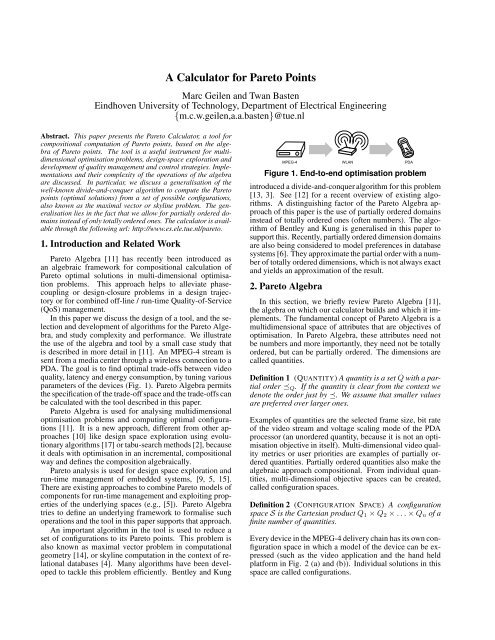
is described in more detail in [11]. An MPEG-4 stream is
sent from a media center through a wireless connection to a
PDA. The goal is to find optimal trade-offs between video
quality, latency and energy consumption, by tuning various
parameters of the devices (Fig. 1). Pareto Algebra permits
the specification of the trade-off space and the trade-offs can
be calculated with the tool described in this paper.
Pareto Algebra is used for analysing multidimensional
optimisation problems and computing optimal configurations
[11]. It is a new approach, different from other approaches
[10] like design space exploration using evolutionary
algorithms [17] or tabu-search methods [2], because
it deals with optimisation in an incremental, compositional
way and defines the composition algebraically.
Pareto analysis is used for design space exploration and
run-time management of embedded systems, [9, 5, 15].
There are existing approaches to combine Pareto models of
components for run-time management and exploiting properties
of the underlying spaces (e.g., [5]). Pareto Algebra
tries to define an underlying framework to formalise such
operations and the tool in this paper supports that approach.
An important algorithm in the tool is used to reduce a
set of configurations to its Pareto points. This problem is
also known as maximal vector problem in computational
geometry [14], or skyline computation in the context of relational
databases [4]. Many algorithms have been developed
to tackle this problem efficiently. Bentley and Kung
Figure 1. End-to-end optimisation problem
introduced a divide-and-conquer algorithm for this problem
[13, 3]. See [12] for a recent overview of existing algorithms.
A distinguishing factor of the Pareto Algebra approach
of this paper is the use of partially ordered domains
instead of totally ordered ones (often numbers). The algorithm
of Bentley and Kung is generalised in this paper to
support this. Recently, partially ordered dimension domains
are also being considered to model preferences in database
systems [6]. They approximate the partial order with a number
of totally ordered dimensions, which is not always exact
and yields an approximation of the result.
2. Pareto Algebra
In this section, we briefly review Pareto Algebra [11],
the algebra on which our calculator builds and which it implements.
The fundamental concept of Pareto Algebra is a
multidimensional space of attributes that are objectives of
optimisation. In Pareto Algebra, these attributes need not
be numbers and more importantly, they need not be totally
ordered, but can be partially ordered. The dimensions are
called quantities.
Definition 1 (QUANTITY) A quantity is a set Q with a partial
order Q. If the quantity is clear from the context we
denote the order just by . We assume that smaller values
are preferred over larger ones.
Examples of quantities are the selected frame size, bit rate
of the video stream and voltage scaling mode of the PDA
processor (an unordered quantity, because it is not an optimisation
objective in itself). Multi-dimensional video quality
metrics or user priorities are examples of partially ordered
quantities. Partially ordered quantities also make the
algebraic approach compositional. From individual quantities,
multi-dimensional objective spaces can be created,
called configuration spaces.
Definition 2 (CONFIGURATION SPACE) A configuration
space S is the Cartesian product Q1 × Q2 × . . . × Qn of a
finite number of quantities.
Every device in the MPEG-4 delivery chain has its own configuration
space in which a model of the device can be expressed
(such as the video application and the hand held
platform in Fig. 2 (a) and (b)). Individual solutions in this
space are called configurations.

Definition 3 (CONFIGURATION) A configuration ¯c = (c1,
c2, . . . , cn) is an element of configuration space Q1 × Q2 ×
. . . × Qn. We use ¯c(Qk) or ¯c(k) to denote ck.
Sets C ⊆ S of configurations represent different options for
realising a particular system or component and how well
they meet objectives. For the MPEG-4 encoder, a configuration
characterises the video quality and bit rate of a stream
encoded with particular parameter settings. An order on
these configurations is induced from the order on the individual
quantities by a point-wise ordering.
Definition 4 (DOMINANCE) If ¯c1, ¯c2 ∈ S, then ¯c1 ¯c2 iff
for every Qk of S, ¯c1(Qk) Qk ¯c2(Qk). If ¯c1 ¯c2, then ¯c1
is said to dominate ¯c2. The irreflexive variant of is ≺.
Dominance of one configuration over another is a partial
order which expresses the fact that the configuration is at
least as good, because it is at least as good in each of the
individual aspects 1 .
Typically, we want to remove elements that do not contribute
interesting realisation options. A configuration that
is strictly dominated by another one is not interesting. Sets
of configurations that cannot be reduced without sacrificing
potentially interesting realisations are called Pareto minimal
(Pareto optimal, Pareto efficient).
Definition 5 (PARETO MINIMAL) A set C of configurations
is Pareto minimal iff for any ¯c1, ¯c2 ∈ C, ¯c1 ≺ ¯c2.
Minimality states that a set of configurations does not contain
any strictly dominated configurations. Configurations
in a set that are not strictly dominated by any other configuration,
are called Pareto configurations or Pareto points.
Pareto Algebra manipulates sets of configurations in
their respective configuration spaces.
Definition 6 (ALGEBRAIC OPERATIONS) Let C and C1 be
configuration sets of space S1 = Q1 × Q2 × . . . × Qm and
C2 a configuration set of space S2.
• min(C) ⊆ S1 is the set of Pareto configurations of C.
• C1 × C2 ⊆ S1 × S2 is the (free) product of C1 and C2.
• C ∪ C1 ⊆ S1 is the set of alternatives of C and C1.
• C ∩ C1 ⊆ S1 is the C1-constraint of C 2 .
• C ↓ k = {(c1, . . . , ck−1, ck+1, . . . , cm) | (c1, . . . , cm)
∈ C} ⊆ S1 ↓ k = Q1 ×. . .×Qk−1 ×Qk+1×. . .×Qm
is the k-abstraction of C.
A central operation is minimisation (min(C)). It reduces
a set of configurations to only its Pareto points. The basic
operators to compositionally construct complex configuration
spaces are the free product (×) and alternative (∪).
The free product combines sets of configurations from different
spaces, typically the first step in combining models.
1 In the literature (e.g., [7]), the dominance relation is sometimes called
weak dominance and the term strict dominance is used when a configuration
is better in all quantities.
2 To be useful in Pareto Algebra the constraint set C1 is usually required
to be closed under addition of dominating configurations [11], but this fact
has no consequence to this paper.
To model the media center and the wireless transmission
together, we start with the product of each of the individual
models. The alternative combines two sets of configurations
from the same space by set union. It can be used when there
are different ways to realise some required functionality and
each of them has been modelled separately. The constraint
operator (∩) enforces a constraint on the relation between
the quantities of configurations and filters out those that do
not satisfy the constraint. It can be used, e.g., to enforce a
bandwidth limitation on the wireless connection. The abstraction
operator (↓) removes information by discarding
optimisation objectives. Often certain objectives only play
a role in the process of composing different components of
the system and are redundant afterwards.
Two operators are not basic operators of the algebra, but
instead derived in terms of basic operators. For the calculator,
it makes sense to implement them in one operation,
because they involve an expansion of configuration sets followed
by a reduction, which can efficiently be done in one
go. The join operator is identical to the (inner-)join operator
in relational databases. Often some of the objectives
of the configuration spaces are not actually final objectives,
but rather additional information required for compositional
construction of the configuration sets. An example
are MPEG-4 encoding parameter settings. The user doesn’t
care about the parameters, but only about the effect they
have on video quality. The composition of an end-to-end
video delivery configuration only makes sense when the encoder
and decoder are set to identical settings of frame rate
and frame size. The join operator enforces this. It can be
expressed as a free product, followed by a constraint on correspondence
between values of selected quantities. We define
a join on a single quantity; generalisation to multiple
quantities is straightforward. (· denotes concatenation of
tuples.)
Definition 7 (JOIN) Let C1 (C2) be a set of configurations
from configuration space S1 (S2). S1 and S2 include the
unordered quantity Q. The constraint D is defined by
D = {¯c1 · ¯c2 | ¯c1 ∈ S1, ¯c2 ∈ S2, ¯c1(Q) = ¯c2(Q)}.
join(C1, C2, Q) = (C1 × C2) ∩ D.
The producer-consumer operator is also a derived operator
combining a free product with a constraint. It occurs
when the use and the availability of certain resources need
to be matched. In the MPEG-4 example this is the bit rate
required by the stream and provided by the wireless transmission,
or the computational power provided by the PDA
processor and required by the decoder running on that processor
(Fig.2(c)). More production of the resource and less
consumption of the resource are considered better. This is
captured by a monotonically decreasing function f relating
the produced quantity to the consumed quantity.
Definition 8 (PRODUCER-CONSUMER CONSTRAINT) Let
C1 (C2) be a set of configurations from configuration space
S1 (S2). Let Q1 be a designated quantity (called the producer
quantity) of S1 and Q2 (consumer quantity) of S2
respectively and f : Q1 → Q2 a monotonically decreasing
function. Let the constraint D be defined by D =
{¯c1 · ¯c2 | ¯c1 ∈ S1, ¯c2 ∈ S2, ¯c2(Q2) f(¯c1(Q1))}.
prodcons(C1, Q1, C2, Q2, f) = (C1 × C2) ∩ D.

§ ¥ ¨
¥ §¡ © ¨
§¨¦§¡ ¤¨
¢¢
¤
¤
¥ §
¢¡¤£¥¡¥¦§©¨
¥ ¤
©
© ¢©
©
©¤ ©
¡¥£¡¥¦§©¨
¥ ¢
¤
§
¤
¤ ¥
¢© ¤
¥¢
Figure 2. Example operations in a video application on a hand held device
3. Implementing the Pareto Algebra
In this section we discuss our implementation of the algebra,
the selection of algorithms and generalisation of existing
algorithms for this tool.
3.1. Data Structure for Configuration Sets
We need a data structure to store large sets (of size N)
of configurations which has efficient procedures for inserting
and removing configurations and for testing whether a
configuration is included in the set (in O(log N)). We have
used the ‘set’ class from the C++ Standard Template Library
(STL)[1]. The set maintains a sorted list of elements
and requires a sorting criterion for configurations. For this
we select lexicographical ordering; per quantity an arbitrarily
total order is used for this sorting.
Many of the algorithms for the Pareto Algebra operators
require sorting of the configurations wrt a particular totally
ordered quantity. To support this, the tool can generate an
index on the set for a particular quantity in O(N log N).
3.2. Complexity of the Operators of the Algebra
We review the complexity of the operators. The
producer-consumer operator is discussed in the next section
and minimisation in Section 5. The free product of a set C1
(size M) and a set C2 (size N) of configurations has M · N
configurations and can be constructed straightforwardly in
O(M ·N ·log(M ·N)). The alternative computes the union
of two sets in O((M + N) · log(M + N)).
The constraint operator is defined as the intersection of
two sets. Practical implementations may have an explicit
representation of the constraint sets. Then the intersection
can be computed directly by a merge. Often however, a constraint
is implemented by a predicate, a characteristic function
which tests (in constant time) whether a configuration
belongs to the constraint set. In both cases the constraint is
computed in O(N log N). Abstraction drops quantities of
the configurations. This is straightforwardly implemented
in time O(N · log N) (removing duplicates is required).
The join operator consists of a product operation followed
by a constraint. A direct implementation of this
definition would first construct the cross product of the
sets, only to remove (typically) many of the configurations
with the constraint. The join is well-known in relational
databases and algorithms are well-studied in that area [8].
The main classes of join algorithms are sort-merge and hash
based algorithms.
We briefly discuss the sort-merge algorithm implemented
in our calculator. Both configuration sets can be
sorted in the dimension on which we want to join, by creating
a sorted index. By merging both sorted lists, the configurations
with matching values for the joined quantity can
efficiently be found. Note that the worst-case complexity of
the join is O(M · N · log(M · N)), since every point may
have the same value for quantity Q. With very few matches,
the algorithm works much more efficiently, converging to
O((M + N) log(M + N)).
4. Producer-Consumer Constraints
An operator that can be implemented more efficiently is
the producer-consumer combination (see Fig 2(a)-(d)). The
straightforward implementation of the mathematical definition
is obtained by first constructing the product of both
spaces, followed by applying the producer-consumer con-

ProducerConsumer(CP , QP , CC , QC, f)
Sort CC on attribute QC, sort CP on attribute QP ;
Let i = 0, j = |CP | − 1;
while i < |CC| and j ≥ 0 do
if CC [i, QC ] f(CP [j, QP ]) then
add CC [i] · CP [j];
i = i + 1;
end
else j = j − 1;
add all CC[k] · CP [j] with k < i;
end
end
if i = |CC| then add all CC[k]·CP [l] with l < j and 0 ≤ k < |CC|;
Algorithm 1: Producer-consumer algorithm
straint as a predicate tested on all its configurations. Although
this implementation achieves the optimal complexity
bound, lots of evaluations of the predicate and construction
of configurations can be saved by a more clever implementation
if the producing and consuming quantities are
totally ordered, which is often the case.
The algorithm (Algorithm 1) explores the border of the
range of feasible and infeasible combinations (see Fig.
2(e)). First, all configurations of the producer are sorted
based on their producing quantity and the configurations of
the consumer on consuming quantity. The algorithm starts
by comparing the worst-case producer (producing the least)
and the best-case consumer (consuming the least, top-left
corner in Fig. 2(e)). If this point is infeasible, it starts increasing
the production (going down in the picture), searching
for a feasible combination. If the point is feasible, it
starts increasing the consumption (going to the right) to find
the first infeasible configuration again. This way the algorithm
traces the border between the infeasible and feasible
regions, knowing that all points below and to the left must
also be feasible combinations. Thus, the number of tests of
the producer-consumer matching, c2(Q2) f(c1(Q1)), is
linear in the sizes of the sets of configurations.
5. Minimisation
The minimisation operator reduces a set of configurations
to only its Pareto points. Vector minimisation algorithms
exist in the literature, although they usually assume
that each of the individual objectives are totally ordered.
This is not true in the case of Pareto Algebra, where the
individual objectives can be partially ordered.
5.1. Simple Cull Algorithm
A straightforward algorithm for minimisation is known
as the Simple Cull (SC) algorithm [16, 14] or as a blocknested-loop
algorithm [4]. The algorithm is shown as Algorithm
2. It looks at the configurations one by one and
maintains a set Cmin of Pareto points among the points observed
so far. Whenever a new point is inspected, two situations
may occur. (i) if the point is dominated by one or
more of the existing Pareto points in Cmin, then the point is
discarded. (ii) if the point is not dominated in Cmin, then
any points from Cmin that are dominated by the new point
are removed and the new point is added to Cmin.
Since every configuration is compared to the configurations
in Cmin, it depends heavily on the size of Cmin how
long the algorithm takes. In the worst case, all configurations
are Pareto points and Cmin grows with every new
SimpleCull(C)
Cmin := ∅;
while C = ∅ do
c := RemoveElement(C); dominated := false;
foreach d ∈ Cmin do
if c d then Cmin := Cmin\{d};
else if d c then dominated := true; break;
end
if not dominated then Cmin := Cmin ∪ {c};
end
return Cmin;
Algorithm 2: Simple Cull minimisation algorithm
point. Hence, the worst-case complexity of the SC algorithm
is O(N 2 ) with N points. In practice the performance
of the algorithm can be much better, depending on the number
of Pareto points in the set. [16] studies the expected
number of Pareto points in a space with configurations with
random numbers and concludes that with a uniform distribution
in a d-dimensional hypercube this number is proportional
to (log N) d−1 . From this, one can argue that the average
complexity of the SC algorithm on problems with a
uniform distribution of points is O(N · (log N) d−1 ). The
behaviour of the algorithm in practical situations depends
strongly on the nature of the design space at hand.
Note that the SC algorithm does not suffer from the fact
that the individual quantities are not totally ordered. One
only needs to be able to perform the test of dominance between
any two configurations to apply it.
5.2. Divide-and-Conquer Minimisation
Although the SC algorithm can give good complexity behaviour
in practice, worst-case complexity is high and may
occur for strongly correlated optimisation objectives [16].
There exists a Divide-and-Conquer (DC) based algorithm,
which improves the worst-case complexity of minimisation
to the average case complexity of the SC algorithm for random
points. Unfortunately, the algorithm only works when
all quantities of the configurations are totally ordered. We
briefly discuss the algorithm, which is due to Bentley and
Kung [3, 13, 14, 16] and in the next subsection we devise
a DC algorithm based on this one that can be applied for
Pareto Algebra.
The essence of the DC approach is to split the set of configurations
in two halves, minimise these sets separately and
merge the results (see Fig. 2(f)). In order to split the sets, an
arbitrary (totally ordered) quantity Q is selected and the set
is sorted wrt that quantity. The median of values is selected
as a pivot and all configurations with values up to the pivot p
are put in one set A and the other configurations, higher than
p, in a set B. The main difficulty of the algorithm lies in the
merging of the results into the Pareto points of the whole
set. All Pareto points in A are Pareto points of the whole
set. Because of the sorting in Q, they cannot be dominated
by points of B. Conversely however, Pareto points in set
B may be dominated by some point from A (e.g., (6,.5) in
Fig. 2(f)). A second recursive algorithm is used to filter out
those points of B that are indeed dominated by points of A.
Details of the algorithm can be found in [3, 4, 13, 14, 16].
The complexity of the DC minimisation algorithm is
O(N ·(log N) d−1 )[3, 16]. It has better worst-case complexity
than the SC algorithm, but also a high overhead because
of the complex recursion. Therefore, it is suggested in [16]

DCMinimize(C)
if |C| < Threshold then return SimpleCull(C);
if exists unordered quantity Q in space of C then
Cmin = ∅;
foreach x ∈ Q do
Cmin := Cmin ∪ UMinimize(C, Q, x);
end
return Cmin;
end
if exists totally ordered quantity Q in space of C then
sort on Q and split in the middle in C L and C H ;
C L min := DCMinimize(CL );
C H
min := DCMinimize(CH );
return DCMarriage(C L
min
end
return SimpleCull(C);
, CH
min , Q);
Algorithm 3: DC algorithm to minimise to Pareto points
to switch to the SC algorithm in the recursive process when
the problem size is small enough.
5.3. Minimisation with P.O. Quantities
In this section, we discuss a practical DC algorithm for
partially ordered quantities. Although the asymptotic complexity
of the DC algorithm cannot be maintained, the algorithm
is efficient for spaces with totally ordered and unordered
quantities and exploits those quantities as much as
possible in the presence of partially ordered quantities.
The DC algorithm splits configurations in two sets according
to the value for a particular dimension. This means
that the approach is not directly applicable to the minimisation
operator of the algebra, because sorting a partial order
(topological sort) is prohibitively expensive (quadratic)
in general. This destroys the worst-case complexity advantage
of the DC algorithm. Still, we observe that in practice
most quantities are either totally ordered, or unordered.
For unordered quantities an alternative efficient divide-andconquer
approach can be defined, which is even more efficient
than the one for a totally ordered quantity. The different
steps are combined in one algorithm (Algorithm 3),
which still achieves the same complexity for only totally ordered
and unordered objectives. It distinguishes four cases.
First, if the problem size is small enough, it uses the SC algorithm.
Second, a DC step is done on an unordered quantity
as long as there is one. Third, DC is tried on a totally
ordered quantity. Fourth, if none of the above is possible,
resort to the SC algorithm 3 .
The algorithm uses a function DCMarriage() to combine
the results of the individual minimisation of separate
sets. The marriage procedure is explained in Fig. 2(f). In
the first step we abstract from the dimension used to separate
the sets A and B (PSNR −1 ), because we know that any
point from A dominates any point from B on that dimension.
Then we need to filter from B those configurations
dominated by configurations from A. If there is another totally
ordered quantity in the space, we split A and B into
respectively AL and AH, and BL and BH according to a
pivot point p in such a way that |AL|+|BL| ≈ |AH|+|BH|.
Then the filtering process can be performed recursively in
three steps. (i) filter all configurations from BL, dominated
by some configuration of AL (here, (6, .5) is filtered out
3 Many additional special cases can be detected and exploited instead of
following through with the basic algorithm. For instance for low number
of dimensions, special algorithms exist.
in the example of Fig. 2(f)), (ii) filter all configurations
from BH, dominated by some configuration of AH, (iii)
filter all remaining configurations from BH, dominated by
some configuration of AL. Note that no configuration from
AH can dominate a configuration from BL. The crux to the
efficiency is that the first two filtering steps involve only half
of the points (|AL ∪ BL| ≈ N
2 , |AH ∪ BH| ≈ N
2
) and the
third step may involve in the worst case almost all N points,
but now the dimension Q can be ignored; any point in AL
dominates any point in BH wrt Q and the problem size is
effectively reduced in that direction. If there is no totally ordered
dimension left, or if the problem size is small enough,
resort to a nested-loop version of the filtering function.
For unordered quantities, a new DC strategy is devised.
The configuration set C is split on dimension Q into classes
Cx for all x ∈ Q and Cx = {¯c ∈ C | ¯c(Q) = x}. (Even if
|Q| = ∞, only a finite number of Cx is non-empty because
C is finite.) Since no configurations from different classes
can dominate each other, the sets Cx can be minimised separately
and min(C) =
x∈Q min(Cx). Moreover, the Cx
can be minimised without regarding the quantity Q. This
is what the function UMinimize() does in the algorithm.
Since the DC on an unordered quantity is simpler and potentially
reduces the number of configurations quicker, the
strategies are applied in the given order. For configuration
spaces with only totally ordered and unordered quantities,
the complexity is still O(N · (log N) d−1 ).
5.4 Performance of minimisation algorithms
To assess the efficiency and scalability of the different
minimisation algorithms, we have performed experiments4 .
A good threshold for switching from the DC algorithm to
SC, has been found to be around 2048 points. Results of
the experiments are shown in Fig. 3. Note that all graphs
are in logarithmic scale on both axes. Fig. 3(a) shows execution
time of the SC and DC algorithms for totally ordered
2D and 4D spaces with uniformly distributed random,
uncorrelated points. SC performs much better than
DC. Fig. 3(b) shows similar measurements for strongly
negatively correlated points (such that all points are Pareto
points.) Here, the DC algorithm is significantly faster, but
the speed difference depends on the number of dimensions.
Fig. 3(c) shows the performance of the SC algorithm with
uniformly distributed random points for different numbers
of dimensions. Complexity increases quickly with the number
of dimensions as the number of Pareto points increases.
Fig. 3(d) compares SC and DC on a space with two ordered
and two unordered quantities, where all points are
Pareto points. Here, the DC algorithm has a clear advantage
over the SC algorithm, because it quickly reduces the problem
with the unordered quantities. The discontinuity in the
graph is caused by the threshold for switching to SC. Additional
experiments with normally distributed random points
show similar results to the uniform distributions even with
moderate (negative) correlation between values.
SC is much more efficient than the DC algorithm when
there is only a small fraction of optimal points. In the other
extreme, when the points are strongly correlated and all
4 All measurements have been performed on a PC with an AMD Athlon
64 processor running at 1.8GHz, with 2Gb of main memory, under the
Microsoft Windows XP OS.

1000
t(s) SC, d=2
SC, d=4
100
DC, d=2
DC, d=4
10
1
0,1
#points
10000,0
0,01
1,0
100 1000 10000 100000 1000000 1000 10000 100000
(a) (b)
1000
10000,0
t(s) SC, d=2
SC, d=4
100
SC, d=6
SC, d=8
10
1
t(s)
1000,0
100,0
10,0
SC, d=2
DC, d=2
SC, d=4
DC, d=4
t(s) SC, d=4
#points
#points
#points
0,1
1,0
1000 10000 100000 1000000 1000 10000 100000
(c) (d)
Figure 3. Efficiency and scalability
points are optimal, the DC algorithm outperforms the SC algorithm.
The presence of unordered dimensions has a positive
effect on the performance of the DC algorithm. From
the experiments it is clear that the overhead of the DC algorithm
over SC is indeed high. For strongly negatively
correlated sets and sets with unordered quantities the DC
algorithm outperforms SC. Such strong correlation can particularly
occur when the sets under consideration are built
compositionally and have been minimised in earlier steps.
6 Other Tool Considerations
The Pareto Calculator is a C++ library with the Pareto
Algebra algorithms and data structures. The library adds
some practical aspects to the basic algebra that improve usability.
A new operator is added, similar to the abstraction
operator, but instead of discarding the information of certain
quantities, it is maintained, but further ignored. This is convenient
when quantities are no longer relevant objectives,
but are still required to identify the configuration’s parameters
setting. This can be used to enforce those parameters on
devices. The operator is called ‘hide’ and makes quantities
invisible to the dominance relation and hence does not take
part in the optimisation process.
On top of this library of Pareto Algebra operators, a user
interface has been made, that can read and write specifications
of components and their trade-offs in the form of XML
files. An XML specification consists of quantity definitions,
definitions of configuration spaces, configuration sets and
a computation section with a sequence of operations to be
performed to compute the result. The tool contains buttons
for the algebraic operators so that computations can also be
done interactively. The calculator is further linked to Microsoft
Excel to make plots of sets of configurations.
7 Conclusions and Future Work
Pareto Algebra has been implemented in a tool presented
in this paper. Selection of algorithms and data structures has
been discussed, an algorithm for the producer-consumer operation
and a novel generalisation of the divide-and-conquer
algorithm for computing Pareto points on partially ordered
domains. Efficiency and complexity of the algorithms has
been investigated experimentally.
1000,0
100,0
10,0
DC, d=4
The design spaces to be explored are often very large
and complexity of the algorithms remains relatively high.
Future work involves the investigation of pruning and approximation
techniques to tackle large spaces. Optimisation
of the calculation query through manipulation of the order
of computation also potentially reduces computation times.
Since Pareto Algebra lends itself well to run-time computation
of trade-offs, it is interesting to investigate the
implications of doing computation on resource-constrained
embedded devices.
Acknowledgement This work is supported by the IST -
004042 project, Betsy.
References
[1] The C++ Standard Template Library. http://www.sgi.
com/tech/stl/index.html.
[2] A. Baykasoglu, S. Owen, and N. Gindy. A taboo search based
approach to find the Pareto optimal set in multiple objective
optimisation. J. of Engin. Optimization, 31:731–748, 1999.
[3] J. Bentley. Multidimensional divide-and-conquer. Communications
of the ACM, 23(4):214–229, April 1980.
[4] S. Borzsonyi, D. Kossmann, and K. Stocker. The skyline operator.
In IEEE Conf. on Data Engineering, pages 421–430,
Heidelberg, Germany, IEEE, 2001.
[5] B. Bougard. Cross-Layer Energy Management in Broadband
Wireless Transceivers. PhD th., Catholic Univ. Leuven, 2006.
[6] C.-Y. Chan, P.-K. Eng, and K.-L. Tan. Stratified computation
of skylines with partially-ordered domains. In SIGMOD ’05:
Proc. of the 2005 ACM SIGMOD international conference on
Management of data, pages 203–214. ACM Press, 2005.
[7] K. Deb. Multi-Objective Optimization Using Evolutionary Algorithms.
Wiley, New York, 2001.
[8] D. J. DeWitt et al. Implementation techniques for main memory
database systems. In Proc. 1984 ACM SIGMOD, pages
1–8, New York, 1984. ACM Press.
[9] W. Eberle, B. Bougard, S. Pollin, and F. Catthoor. From myth
to methodology: cross-layer design for energy-efficient wireless
communication. In Proc. DAC, pages 303–308, 2005.
[10] M. Ehrgott and X. Gandibleux. An Annotated Bibliography
of Multi-objective Combinatorial Optimization. Technical
Report 62/2000, Fachbereich Mathematik, Universität
Kaiserslautern, Kaiserslautern, Germany, 2000.
[11] M. Geilen, T. Basten, B. Theelen, and R. Otten. An algebra
of Pareto points. In Proc. Application of Concurrency to System
Design, 5th Int. Conf., ACSD 2005, pages 88–97, Los
Alamitos, CA, USA, 2005. IEEE Computer Society Press.
(full version to appear in Fundamenta Informaticae, 2007)
[12] P. Godfrey, R. Shipley, and J. Gryz. Maximal vector computation
in large data sets. In VLDB ’05: Proc. 31st Int. Conf. on
Very large data bases, pages 229–240. VLDB Endowment.
[13] H. T. Kung, F. Luccio, and F. P. Preparata. On finding the
maxima of a set of vectors. J. ACM, 22(4):469–476, 1975.
[14] F. P. Preparata and M. I. Shamos. Computational Geometry
- An Introduction. Springer, 1985.
[15] P. Yang and F. Catthoor. Pareto-optimization-based runtime
task scheduling for embedded systems. In Proc.
(CODES+ISSS) 2003, pages 120–125. ACM, 2003.
[16] M. Yukish. Algorithms to Identify Pareto Points in Multi-
Dimensional Data Sets. PhD thesis, Pennsylvania State University,
August 2004.
[17] E. Zitzler and L. Thiele. Multiobjective evolutionary algorithms:
A comparative case study and the strength Pareto approach.
IEEE Trans. on Evolutionary Computation, 3(4):257–
271, November 1999.