dissertation global and local fracture properties of metal matrix ...

MONTANUNIVERSITÄT MONTANUNIVERSITÄT LE LEOBEN LE OBEN
DISSERTATION
GLOBAL AND LOCAL FRACTURE
PROPERTIES OF METAL MATRIX
COMPOSITES
by Dipl. Ing. Ilchat Sabirov
LEOBEN, 2004

Acknowledgements
First of all, I would like to acknowledge gratefully Univ. Doz. Dr. Otmar Kolednik for being a
patient supervisor and for supporting this work with new ideas. I could not have imagined
having a better advisor and mentor for my PhD, and, without his common-sense, knowledge,
kind participation in my work, and support of my research activity, this thesis would not
appear.
I would like to express my deep gratitude to Univ. Doz. Dr. Reinhard Pippan for his
discussions and kind help during execution of this work. His helpful comments and notes are
highly appreciated.
I would like to thank O. Univ. Prof. Dr. Robert Danzer from the Department of Structural and
Functional Ceramics for his kind assent to examine my PhD.
I am indebted to all my colleagues at the Erich Schmid Institute of Materials Science of
Austrtian Academy of Sciences for a friendly atmosphere. My heartfelt thanks to D.I. Klaus
Unterweger, Dr. Cristian Motz, Dr. Ernst Gach, Dr. Hans-Peter Brantner, D.I. Herbert
Kreuzer, Dr. Rene Wadsack, D.I. Andreas Vorhauer, D.I Alois Maier, D.I. Gernot Trattnig,
Mag. Günter Maier, etc., for their kind help in any matter. Special thanks to Franz Hubner,
Günter Aschauer, Edeltraud Haberz, and Gabriele Moser for the excellent preparation of
specimens. I apologize to all colleagues whose names have been unintentionally omitted.
I also wish to thank Univ. Doz. Dr. Heinz Pettermann and Dr. Dominik Duschlbauer from
Vienna University of Technology for their cooperation during execution of this work.
Finally, I would like to express my thanks to Prof. Ruslan Valiev from the Ufa Aviation
University for his encouragement in my research activity.
1
Leoben, April 2004.

TABLE OF CONTENTS
1. Introduction 5
2. Background 7
2.1. Metal matrix composites as advanced materials 7
2.2. The influence of the global microstructure and the matrix condition
on the global mechanical properties in metal matrix composites 8
2.3. The process of void initiation in materials with particles 9
3. A method to estimate the local conditions for void initiation in materials with
inclusions 15
3.1. An automatic fracture surface analysis system 15
3.2. The determination of the CODi- and CODvi–values 16
3.3. Estimate of the maximum principal stresses in both phases 20
3.3.1. Estimate of the HRR stress tensor at the moment of void initation 20
3.3.2. The determination of the maximum stresses both in the particle and in the
matrix by a Mori-Tanaka type mean-field correction 22
3.3.2.1. The Eschelby approach 22
3.3.2.2. Some general mean-field relations 24
3.3.2.3. Solution procedure 25
4. Local fracture properties of metal matrix composites 29
4.1. Materials for investigation and their mechanical properties 29
4.1.1. Cast MMCs 29
4.1.1.1. Materials characterization 29
4.1.1.2. Tensile tests 30
4.1.1.3. Fracture mechanics tests 32
4.1.2. Powder metallurgy MMC 34
4.1.2.1. Materials characterization 34
4.1.2.2. Compression tests 35
4.1.2.3. Fracture mechanics tests 37
4.1.3. The relation between the mechanical properties 37
2

4.2. The effect of the heat treatment on the fracture surface 40
4.3. The effect of the particle location with respect to the crack tip on the local
fracture properties 42
4.3.1. The relation between the particle location with respect to the crack tip
and the CODi-values 42
4.3.2. The relation between the particle location with respect to the crack tip
and the CODvi-values 51
4.4. The maximum particle stresses at the moment of void initiation 56
4.5. The relation between the local conditions for void initiation and global mechanical
properties 64
4.6. Application of Weibull distribution for fractured particles 66
5. The relation between the inclusion size and the local fracture properties 69
5.1. Material and mechanical properties 69
5.1.1. Materials characterization 69
5.1.2. Tensile tests 70
5.1.3. Fracture mechanics tests 70
5.2. The effect of the particle location and the inclusion size on the
CODi- and CODvi-values 71
6. Comparison of the local and global fracture properties 75
7. Application of ECAP to improve the homogeneity of the particle distribution in
MMCs 79
7.1. Material 79
7.2. A model by Tan and Zhang for the case of combination of extrusion
and ECAP 80
7.3. A quadrat method to estimate the homogeneity of the particle distribution
in MMCs 83
7.4. The effect of ECAP on the particle distribution, the global, and local
fracture properties in MMCs with severe clustered particle distribution 85
7.4.1. The effect of ECAP on the microstructure 85
7.4.2. The effect of ECAP on the global fracture properties 88
7.4.3. The effect of ECAP on the fracture surface morphology 90
3

7.4.4. The effect of ECAP on the local fracture properties 92
7.5. About possible application of ECAP to improve the particle distribution
in different MMCs 96
8. Summary 98
9. Appendix 101
References 155
4

1. Introduction
Section 1
In spite of the attractiveness of metal matrix composites (MMCs) because of their advantages,
such as increased strength, stiffness, and modulus, their low fracture toughness in comparison
with the fracture toughness of the matrix material is a primary obstacle against their
widespread application in materials engineering. Many investigations have been already
devoted to the mechanical behavior of MMCs and its relation to the microstructure, but both
the microstructure and the properties have been considered at the global level: the variation of
strength and fracture toughness, measured by conventional tensile and fracture mechanics
tests, have been studied as a function of parameters, such as the particle volume fraction, the
average particle size, the particle shape, the mean particle orientation with respect to the crack
plane, etc. [1-5].
In comparison to previous investigations, the idea of this work is to study experimentally the
local fracture properties: the conditions for void and fracture initiation. The motivation to
study it is explained in Section 3.
A method to estimate the local conditions for void initiation near the crack tip and the position
of the particle location with respect to the crack tip is developed. The main tool of this method
is a quantitative analysis of the fracture surfaces via automated stereophotogrammetry. By this
tool, the local crack tip opening displacement at the moment of fracture initiation, CODi, (a
measure of the local fracture initiation toughness) and the crack tip opening displacement at
the moment of the void initiation, CODvi, (which can be considered as a local void initiation
toughness) are determined. From the local void initiation toughness, the maximum normal
stresses in the particles and at the interface at the moment of void initiation are evaluated by
means of the HRR-field theory, a Mori-Tanaka type mean field analysis, and according to the
model by Argon et al. This method is described in details in Section 4. The method is applied
to Al6061 based MMCs. The results of investigation are presented and discussed in Sections 5
and 6. The procedure is also applied to MnS-inclusions in the mild steel St37 (Section 6).
Another topic of our investigations is an improvement of the homogeneity of particle
distribution in MMCs reinforced by small (less than 10 µm) particles. As known, these
materials are prone to cause an inhomogeneous particle distribution. A method for equal
channel angular pressing (ECAP) is proposed to solve this problem. The effect of ECAP on
the homogeneity of the particle distribution in an Al6061-20%Al2O3 MMC processed by
powder metallurgy (PM) technology on the global and local fracture properties near the crack
tip is investigated by automated stereophotogrammetry (Section 7).
5

Section 1
The main results of this investigation are following: the local fracture properties are
influenced by the particle location with respect to the crack tip, the particle size, the material
strength. A correlation between the local and global fracture properties is found.
It should be noted that this work a part of the research devoted to the local deformation and
fracture properties of MMCs performed in frames of the FWF-project P14333-PHY.
6

2. Background
Section 2
2.1. Metal matrix composites as advanced materials
The development of MMCs for structural application is relatively new; it started
approximately 20 years ago. The objectives of these developments are usually improvement
of the performance of components, weight reduction, and replacement of more expensive
conventional alloys. A vast amount of publications devoted to these problems prove the
importance of composite materials in modern technology.
Currently produced and practically applied are composite materials based on light metal
alloys, especially on aluminum, magnesium, and titanium, as well as on copper and high
temperature superalloys reinforced by stable ceramic dispersion particles. Composite
materials based on light metal alloys are reinforced with dispersion particles, platelets, short
and continuous fibers and have very good mechanical properties. For instance, the MMCs on
magnesium basis reinforced by SiC particles have mechanical properties which are by 30-
40% better in comparison with the unreinforced magnesium alloys. Such MMCs are applied
in the aircraft and car technology (space, satellite, and antenna structures) [1]. The advantages
of aluminum composite materials, such as a high resistance to wear, a good strength, and a
relatively good heat conduction, has resulted in their practical application in the car industry
(discs of car brakes, Cardan shafts in passenger cars) [6], and in aerospace engineering
(helicopter structures, jet engine fan blades) [1]. Titanium based composites have found a
wide application as materials for high temperature structures [6]. Copper based composite
materials, having a good heat conductivity, a good wear resistance, and an ability to join with
metal alloys or special ceramics, are used in electronics as electrical contacts, resistance
welding electrodes, elements of electronic system [6]. Nickel based superalloys have better
high temperature mechanical properties than conventional high temperature alloys. Therefore,
they are applied in jet engine technology and industrial turbines (as high temperature engine
components, rotors for compressions, etc.) [1, 6].
The industrial application of MMCs has been developing, and new composite materials have
been offered to industry by researchers. It is clear that detailed investigations devoted to the
mechanical and physical properties of these materials must precede their industrial
application. In the next section, a short review of relations between the composite architecture
and mechanical properties is given.
7

Section 2
2.2. The influence of the global microstructure and the matrix condition on the global
mechanical properties in metal matrix composites
The influence of the global microstructural parameters such as the particle volume fraction,
the average particle size, etc., on the global mechanical properties has been already
investigated in detail. The experimental results can be roughly generalized as follows [7]:
With increasing particle volume fraction, the yield strength and the ultimate tensile strength
increase, the ductility and the fracture toughness decrease, e.g., [8]. For a constant particle
volume fraction, the tensile strength tends to increase with decreasing particle size, e.g.,
[9,10]. No such simple pictures have been found for the more complex properties fracture
toughness and fatigue resistance; ambiguous results have been reported here [7, 11-12].
Stronger matrix alloys produce stronger composites, e. g. [13,14]; the increase in strength due
to the reinforcement decreases with increasing matrix strength; in the case of very high
strength alloys, reinforcements may even lead to a reduction in strength [15]. Therefore, one
of most important factors affecting the mechanical properties of MMCs is the heat treatment.
In [16], the effect of the heat treatment on mechanical properties of the PM-MMC Al7093-
15%SiC was investigated. An increase of the yield strength with increasing aging time up to
the peak aged condition was found. A further increase of aging time led to a slight decrease of
the yield strength. The dependence of the fracture strain and the strain hardening coefficient
on the aging time demonstrated an opposite character. A good correlation between the
fracture strain and the strain hardening coefficient was found. It was shown that the fracture
toughness has an inverse dependence on strength and correlates well to the strain hardening
coefficient. Fracture surface inspection revealed the dominance of the particle fracture for the
solution treated, under-aged, peak-aged, and slightly over-aged conditions of the matrix
whereas, in the highly overaged condition, (near-)interface debonding failure dominated.
In [17], a model was proposed to predict the fracture toughness in this material. This model is
based on a prediction proposed by Hahn and Rosenfield [18],
8
1
2
1 ⎡
⎤ 1
3 −
⎢ ⎛π
⎞
6
= 2σ
E⎜
⎟ d⎥
f . (2.1)
⎢ ⎝ 6 ⎠ ⎥
⎣
⎦
K IC
y
In Eq. 2.1 σy is the yield strength of material, E the Young modulus, d the particle size, and f
the particle volume fraction. It was shown in [17] that Eq. 2.1 significantly overestimates the

Section 2
fracture toughness data. Using the analyses of Rice and Johnson [19] and Shih [20], Pandey et
al. proposed a modified interpretation of the Hahn and Rosenfield model
K
c
9
1
2
⎡ βσ y Ed ⎤
= 0.
77 ⋅ ⎢
2 ⎥ f
⎣d
n ( 1−
v ) ⎦
1
−
6
, (2.2)
where β = 0.5, dn is a dimensionless constant depending on the strain hardening coefficient
[20], and v is the Poisson ratio. This prediction has provided a better agreement with fracture
toughness data for this material.
In [21], the effect of the aging process on the properties of an Al6061 alloy reinforced by 20%
of Al2O3 particles was studied. A similar dependence of mechanical properties on the heat
treatment condition was revealed as in [16]. A shift from particle fracture to an interface (or
near-interface) decohesion when moving from the underaged to the overaged regimes, and
higher local volume fraction of spinel products at the particle/matrix debonded interface of
overaged specimens were observed.
The plastic deformation behavior of MMCs was investigated in [22]. It was shown that, in an
Al6061-SiC MMC in under-aged condition, plastic strain is distributed homogeneously
throughout the whole length of the specimen, whereas strain localization is noted for the
MMC in the peak-aged condition [22]. This difference is also reflected in the damage
mechanism. In the under-aged condition, the particle cracking increases with strain over the
whole length of the specimen, and the density of cracked particles near the fracture surface is
comparable to that in the rest of the specimen. In the peak-aged condition, the extent of the
particle cracking is less than in the under-aged condition and tends to be highest near the
fracture surface. The percentage of cracked particles is less than about 5% of the total particle
content, and experiments show that the fracture strain can be recovered after pre-strain levels
which produce extensive particle fracture. The fracture strain is very sensitive to heat
treatment, decreasing with increasing strength and decreasing strain hardening coefficient, so
the matrix condition is very important in the fracture process [22].
2.3. The problem of the homogeneity of the particle distribution and its influence on the
mechanical properties
A poor reinforcement distribution restricts the application of MMCs in industry due to the
degraded mechanical properties and limited formability. As well known, in order to gain a

Section 2
high strength, fine reinforcements and a relatively large particle volume fraction are preferred
[2]. However, it is difficult to take advantage of both of these requirements because they are
prone to cause an inhomogeneous particle distribution [23].
A number of studies have shown that during the deformation of particulate reinforced MMCs
there is a progressive development of damage within the material. It has been observed that
the damage tends to originate preferentially in particle clustered regions [24, 25]. Thus, one of
the most important microstructural features of the MMCs is the spatial distribution of the
particles. In [26, 27], an Eshelby based approach was used to create a model of a clustered
composite. A composite with non-uniform particle distribution was considered as a two phase
material comprising regions of higher than average local volume fraction as stiffer regions
within a more compliant dilutely reinforced matrix. This analysis suggests somewhat
surprisingly, that a composite containing clustered particles should have a higher flow stress.
It was also found that larger stresses may be expected in both the matrix and particles in
clustered regions compared with a composite containing a homogeneous particle distribution.
On the other hand, it is suggested in [28] that reinforcement clustering tends to reduce the
composite flow stress, relative to an equi-spaced array. Zhiru et al. [29] have proposed that
the matrix triaxial stresses are generally higher in clustered regions of four or more particles,
thus shielding the center of the cluster from plastic flow due to the higher local levels of
constraint imposed on the matrix. Plastic flow is, thus, only expected in the center of the
clusters once the more dilutely reinforced regions of the matrix have become sufficiently
work hardened. In [30], a decrease of experimentally determined global fracture toughness
with increasing degree of clustering was observed.
2.4. The process of void initiation in materials with particles
As well known, micro-ductile fracture consists of three stages: void nucleation, void growth,
and void coalescence [31]. In ductile materials reinforced with hard second phase particles,
void nucleation occurs either by particle/matrix decohesion or the particle fracture
mechanism. Void nucleation can determine the ductility, since the subsequent stages of void
growth and coalescence can be extremely rapid (especially in the case of large ceramic
particles) once the void initiation has occurred. Therefore, the full understanding of void
initiation process is very important to predict the fracture properties of MMCs.
10

Section 2
An energy criterion and a stress criterion have been suggested to characterize the
particle/matrix interface separation [32]. A detailed analysis by Tanaka et al. [32] has shown
that for particles having a size smaller than 250 Å, the particle/matrix separation is primarily
controlled by the energy criterion. In this case, the particle/matrix separation will occur when
the elastic strain energy which is released upon decohesion becomes equal to the newly
created surface energy. When an inclusion is larger than 250 Å, the energy criterion is always
fulfilled and the particle/matrix separation is primarily controlled by the stress criterion [32].
Void nucleation occurs at the attainment of a critical normal stress at the particle/matrix
interface.
Some models based on a dislocation theory were developed. Ashby proposed a model where
primary deformation incompatibilities do not produce cavities directly, but initiate highly
organized secondary dislocation loops from the interface of the inclusion with the matrix to
reduce the local shear stresses [33]. These loops can form reverse pile-ups and can build up
increasing interfacial stresses until they reach the interfacial strength. In [31], the local stress
on the particle interface has been estimated as a function of the local dislocation density
around a particle. It was demonstrated that the rate of dislocation storage around a particle, in
a plastically deforming matrix, decreases with an increase in particle size and, above a critical
particle size of 1 µm, a continuum plasticity model can be applied to describe the microvoid
nucleation process, since the local strain hardening effect around the particle is of the same
magnitude as that in the matrix.
Argon et al. [34] used a continuum mechanics theory to estimate the maximum interfacial
stresses. They considered a rigid cylindrical inclusion embedded into an incompressible
power-law hardening material subjected to a pure shear deformation. The actual behavior of
the material is bounded by two limiting idealizations: a rigid ideally plastic behavior and a
linear behavior. The stress concentrations obtained for these two extreme idealizations were
compared to estimate the actual interfacial stresses. It was shown that the maximum
interfacial stresses can be calculated as a sum of the von Mises equivalent stress, σeq, and the
hydrostatic stress, σm,
σ interf max = σeq + σm. (2.3)
In [35], Argon and Im investigated the behavior of equiaxed Fe3C particles in a 1045 Steel,
Cu-Cr particles in a Cu-0.6%Cr alloy, and TiC particles in a maraging steel. Cylindrical
tensile specimens with and without machined notches were tested up to failure. The broken
specimen halves were sectioned along the axis, metallographically polished, and lightly
11

Section 2
etched to mark the inclusions. The inclusions which have initiated voids were detected, and
the number of voids was plotted as a function of the distance from the fracture surface. The
point along the axis where the void density drops to zero was taken as characterizing the
critical conditions for interface separation. A finite element analysis was performed, [36], to
compute the stress conditions at this point. The critical interfacial stresses were then
calculated according to Eq. (2.3). The maximum interfacial stresses were 1670 MPa, 990
MPa, and 1820 MPa for Fe3C, Cu-Cr, and TiC particles, respectively.
Arsenault and Flom evaluated the interfacial strength between particles and the matrix in an
Al6061 based MMC with 1% SiC particles [37]. Specimens similar to that used in [35] were
machined and procedure used in [35] was applied to the specimens. The interfacial strength
was calculated by Eq (2.3), taking into account the stress triaxiality for the tip of the notch,
where the triaxiality reaches its maximum. The interfacial strength was determined as 1690
MPa. This result does not seem to be correct, since the number of voids associated with the
debonding of SiC particles was much smaller than the total number of voids related to the
fracture. A few examples of the areas where debonded SiC particles are located were
observed, but they were distant from the tip of the notch.
Beremin [38] studied the conditions for void initiation for elongated MnS inclusions in a low
alloy steel A508. Notched tensile specimens were loaded to different global deformations and
subsequently sectioned and polished to determine the outer boundary of the region within
which voids have been initiated. The local stresses at this boundary were computed with a
finite element analysis, and the maximum principal stress in the inclusion at the moment of
void initiation evaluated by the equation
σ p max =σm + (2/3+λ)σeq. (2.4)
This equation was deduced from a non-linear Eshelby-type approach, following [39]. The
parameter λ is a function of the particle shape; λ = 1 for a spherical particle. Beremin found
that the σ p max-values for the MnS-inclusions in the steel A508 are temperature independent,
but depend on the specimen orientation: σ p max = 1120±60 MPa in the longitudinal direction,
where MnS-inclusions are fractured, and σ p max = 810±50 MPa in the short transverse
direction, where MnS-inclusion/matrix decohesion prevails.
Toda et al. [40] determined the fracture strength of second-phase particles in a notched 3-
point bend specimen made of a wrought Al-Li alloy. A side-surface of the specimen was
polished and etched before the testing. An interrupted in-situ loading experiment was
12

Section 2
conducted in the scanning electron microscope (SEM). The notch radius was 150 µm. The
position and size of each particle was measured within a region of 500 µm around the notch
and the extending crack tip. The chemical composition of the inclusions was determined by a
SEM-EDX analysis. After each loading step, a micrograph was taken to detect the broken
particles. From the value of the J-integral, J, the particle fracture stress was evaluated using
the stress field approach proposed by Hutchinson [41], Rice, and Rosengren [42] (HRR-
theory) and a mean field correction following Tanaka et al. [32]. The process zone where
large deformations appear directly at the growing crack tip was excluded from the analysis.
Toda et al. found values of the maximum normal stress of σ p max = 710 MPa for CuAl2 and
Al2CuMg particles with diameters between 5 and 8 µm. Whereas the fracture strength of the
CuAl2 particles did not change much with increasing particle size, larger Al2CuMg particles
exhibited considerably smaller values, e.g., σ p max = 540 MPa for diameters between 14 and
18 µm. Al3Zr and Al3Ti particles did not fracture, thus a lower limit of their fracture strength
could be determined: σ p max ≥ 1000 MPa and 910 MPa, respectively.
The study of Toda et al. is remarkable, however, a few disadvantages has prevented the direct
application of the procedure for our materials:
(1.) The HRR-field is, strictly speaking, not applicable for a region around a notch, nor is
it for a growing crack. Regarding the growing cracks, Toda et al. claim that the HRR-
field should be still valid if a parameter Ω = Eεfr /σy is smaller than 34.5 (E is the
Young modulus, εfr denotes the fracture strain in a uniaxial tensile test, and σy the
yield stress). Hereby, Toda et al. refer to a paper by Chan [43] who used the
parameter Ω to distinguish between stable and unstable crack growth regimes. As has
been shown by Hutchinson and Paris [44], the conditions of J-controlled crack
growth will be lost for any material, if the crack extension becomes too large.
Moreover, it is demonstrated in [44] that a tough material, where dJ/da and the
parameter Ω are large, will exhibit J-control for a longer regime of crack extension
than a less tough material with a small Ω.
(2.) The mean-field analysis was performed assuming an inclusion in a matrix under a
uniaxial tensile stress. A particle near a crack tip will, however, experience a highly
triaxial stress state.
(3.) The measurement at the side surface of the specimen might be not representative for
the bulk behavior. It is well known that, because of the lower constraint, void
initiation and void growth are retarded near the side surface compared to the
midsection region.
13

Section 2
(4.) The specimen preparation might pre-damage some of the particles so that they fail at
a lower stress.
As one can see, despite a large number of investigations dealing with the fracture behavior of
MMCs, the local fracture properties in MMCs have not been investigated so far, probably,
due to the absence of appropriate tools. But this topic is very important for inhomogeneous
materials. As the void initiation is the first stage of the ductile fracture, the conditions for void
nucleation call great interest, especially, near the crack front in the interior of the specimen.
As shown in next section, an application of recently developed tools for fracture surface
analysis could solve such a problem as the impossibility to investigate the fracture processes
in the interior of the specimen and give a possibility to determine the local conditions for void
initiation for individual particles near the crack tip.
14

Section 3
3. A method to estimate the local conditions for void initiation in materials
with inclusions
This section describes the proposed procedure to estimate the local conditions for void
initiation near the crack tip. The procedure consists of:
1) For individual particles lying in the midsection region near the crack tip, the values of the
crack tip opening displacement at the moment of void initiation, CODvi, are determined.
This is done by using stereophotogrammetry and a digital image analysis system.
2) The mesoscopic stress tensor at the position of each considered particle is estimated by the
HRR-theory from the determined CODvi-value.
3) The stress tensors in both the particle and in the matrix are calculated by a non-linear
Mori-Tanaka secant approach.
Below, each step is outlined in detail.
3.1. An automatic fracture surface analysis system
To determine the values of the crack tip opening displacement at the moment of void
initiation, CODvi, and at the moment of fracture initiation, CODi, as well as the polar
coordinates of the particle location with respect to the crack plane, an automatic fracture
surface analysis system is used [45, 46]. The key part of this system is a matching algorithm
which is able to find automatically homologue points in a stereo image pair which is taken in
a scanning electron microscope (SEM). Homologue points are points in the two images which
belong to the same physical point on the specimen. The stereo image pair is produced by
tilting the specimen in the SEM. Each image consists of 1024 x 768 pixels at 256 gray levels.
On average, between 20000 to 30000 homologue points are found. It should be noted that
images with a resolution of up to 4000x3200 pixels can be taken in new SEMs. For such
pictures, the number of homologue points may increase by a factor 10 or more.
From the homologue points and the three image parameters, magnification, working distance,
and tilt angle, a three-dimensional model of the depicted fracture surface region is generated,
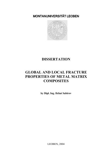
called “digital elevation model” (DEM). In Figure 3.1, a DEM for a cast Al6061-10%Al2O3
MMC is given as an example. The DEM can be cut arbitrarily to extract fracture surface
15

Section 3
Fig. 3.1. The digital elevation model of a cast Al6061-10%Al2O3 MMC.
profiles. Further important capabilities of the automatic fracture surface analysis system are
the automatic evaluation of profile and surface roughness parameters and the determination of
fractal dimensions [47].
The first version of the automatic fracture surface analysis system used a simple matching
algorithm, based on the evaluation of a cross-correlation coefficient [48]. Later, the system
has been completely modified with respect to the matching algorithm and the user interface
[46]. A comprehensive description of the principles of the new matching algorithm is given in
[49]. Both systems have been applied successfully to analyze ductile and cleavage fracture
surfaces of metals [50, 51], metallic glasses [52], and intermetallic alloys [53], but it has been
also proven valuable for the inspection of the surface structure of many classes of materials,
from metals to biological materials.
In the following section, it is described how the automatic fracture surface analysis system is
applied to determine the local CODi- and CODvi-values in materials with inclusions.
3.2. The determination of the CODi- and CODvi –values
The SEM-micrographs of Figure 3.2 show corresponding regions near the midsection on the
two halves of a broken compact tension (CT) specimen made of a cast Al6061-10%Al2O3
16

Section 3
Fig. 3.2. Corresponding stereo image pairs with profiles passed through a particle
(the particle location is marked).
MMC. The pre-fatigue regions (in the bottom part of pictures) and the regions of micro-
ductile fracture can be clearly distinguished. From the DEMs of the corresponding regions,
crack profiles are extracted perpendicularly to the pre-fatigue crack front. The profiles are
drawn so that they cross an alumina particle in front of the crack tip. Sometimes, the paths
have a zigzag shape to find easier the corresponding path on the second specimen half.
In Figure 3.3a, the two corresponding profiles through an alumina particle of the specimen are
arranged so that the moment of fracture initiation is depicted, i.e., the moment when the
ligament between the first void in front of the tip and the blunted pre-crack fails. The upper
profile (drawn as the red line) corresponds to the left-hand side of Figure 3.2, the lower
profile (blue line) corresponds to the right-hand side. The location of the particle in the center
of the void is marked. The critical crack tip opening displacement, CODi, which is a measure
of the local fracture initiation toughness [50], can be determined: CODi = 17 µm.
If the lower profile of Figure 3.3a is shifted vertically so that two profiles touch each other at
the location of the marked particle, we get a sketch of the crack at the moment of void
initiation (Fig. 3.3b) and the crack tip opening displacement at the moment of void initiation,
CODvi, can be measured. For the considered particle, we get CODvi = 10 µm. Analogously to
17

height [µm]
height [µm]
10
0
-10
-20
-30
10
0
-10
-20
-30
COD i =17µm
Section 3
-60 -20 20 60 100
COD vi=10µm
distance [µm]
a)
-60 -20 20 60 100
distance [µm]
b)
18
r
Θ
particle
Fig. 3.3. Crack profile through a particle in the cast Al6061-10%Al2O3 MMC: a) at the
moment of fracture initiation; b) at the moment of void initiation at the particle location.
the local fracture initiation toughness CODi (which can be transferred to critical values of the
stress intensity or the J-integral), CODvi gives the resistance of the material against void
initiation and, thus, it can be considered as a local “void initiation toughness” [54].

Section 3
The location of the particle center with respect to the crack tip, given in polar coordinates (r,
θ), is also determined from the crack profile. The polar coordinates of the particle center shall
be measured from the initial position of the tip of the fatigue pre-crack before the blunting
process starts. This can be performed more accurately from the crack profiles depicting the
moment of void initiation, Figure 3.3b. For many materials, the tip of the fatigue pre-crack
can be found on the SEM micrographs as the beginning of the stretched zone.
As follows from the procedure (parallel shifting of profiles), the method of determination of
CODvi is based on the assumption that the void growth rate in a direction perpendicular to the
crack plane,
.
R , is equal to the COD growth rate,
y
19
.
COD .
An early numerical analysis of void growth near a crack tip, [55], suggests that the COD
growth rate should be several times higher than the void growth rate. If this would be valid,
we would get negative CODvi-values for most of the considered below particles, so that we
conclude that this cannot be true. In [56], the growth of a single void near the crack tip was
investigated for different specimen geometries by the finite element method. In Figure 3.4, the
Fig. 3.4. Plots of the crack tip opening displacement, B, the dimension of the void size in two
directions, Rx and Ry, and the size of the ligament between the crack tip and the void , D, in
plane strain case (taken from [56]).
i

Section 3
Fig. 3.5. The observations of the growth of an assemble of voids near the crack tip for plane
strain conditions (taken from [57]).
void size in two directions, Rx and Ry, the size of the ligament, D, the value of the crack tip
opening displacement, B, are plotted as a function of the dimensionless loading parameter of
the crack,
J
σ
o o R
, for different specimen geometries: the double-edge cracked (DEC), the
center-cracked plain (CCP), three point bending (TPB), and the single-edge cracked (SEC).
From Figure 3.4, the void and COD growth rates can be estimated for a TPB specimen (which
has very similar constraint conditions as a compact tension specimen) and for plane strain
conditions. The result is
.
.
COD ≈ 1. 1⋅
D . It should be noted that results obtained for other
specimen types differ: for instance, for the SEC specimen,
20
.
CODi .
≈ 3⋅ D . In a recent study,
[57], the growth of an assemble of voids in a polycrystalline microstructure near a crack tip
has been modeled. An analysis of Figure 3.5 shows again that the void and COD growth rates
are approximately equal. Thus, it can be concluded that the inaccuracy of determination of the
CODvi-values related with the simple shifting of profiles is not high.
3.3. Estimate of the maximum principal stresses in both phases
3.3.1. Estimate of the HRR-stress tensor in the moment of void initiation
The stress tensor at the moment of void initiation is estimated from the HRR-field solution
(Eq. 3.1) which gives the stress field around a crack tip as a function of the global material
properties and the polar coordinates with respect to the crack tip (Fig. 3.6) [41, 42],

Section 3
Fig. 3.6. Schematic view of the HRR-theory.
21
(3.1)
In Eq. 3.1, E is the Young modulus, J is the fracture toughness of material, σ0 is the yield
strength, r and θ are the polar coordinates, IN and dN are dimensionless constants both
depending on the strain hardening coefficient, N, and on σ0 /E, ~ σ ( N,
θ ) is a dimensionless
function listed in [59].
The J-integral in Eq. 3.1 can be substituted by COD using the relation proposed by Shih in
[58]
, (3.2)
where dN is dimensionless constant depending on the strain hardening coefficient, N, [58].
The material is assumed to follow a standard power-law work hardening behavior
, (3.3)
where according to [59], the σ0 is set to the yield strength, σy, and α is determined from the
tensile true stress-strain curve.
⎡ E J ⎤
σ σ
~
ij = 0 ⎢
σ ,
2 ⎥
ij
⎢⎣
ασ 0 I N r ⎥⎦
J =
d
1
σ 0
N
To evaluate the stress tensor at the moment of void initiation, σ HRR vi, the measured r, θ, and
the CODvi-values are inserted into Eqs. (3.2) and (3.1). From the stress tensor σ HRR vi, the
maximum principal stress, σ HRR max, can be calculated.
1/(
N + 1)
COD
ε
⎛ σ ⎞
= α ⎜
⎟
ε 0 ⎝σ
0 ⎠
N
r
θ
( N θ )
ij
σij

Section 3
3.3.2. The determination of the maximum stresses both in the particle and in the matrix by
a Mori-Tanaka type mean-field correction
So far, the material has been considered as a material with homogenized properties. The
considered length scale is called the “mesoscopic scale” and the stresses are denoted as
“mesoscopic stresses”, i.e., the HRR-stresses are meso-stresses. However, for the evaluation
of local phenomena, such as particle failure, the “microscopic scale” has to be considered. To
do this, a non-linear Mori-Tanaka type mean field approach is applied which is based on the
Eshelby theory. In the next section, the Eshelby approach is presented in detail.
3.3.2.1. The Eshelby approach
Internal stresses are present in any inhomogeneous material consisting of several phases.
They arise as a result of some kind of misfit between the constituents (matrix and the
reinforcement). Such a misfit could arise from a temperature change when the constituents
have different thermal expansion coefficients, but a closely related situation is created during
mechanical loading – when a stiff inclusion tends to deform less than the surrounding matrix.
Analysis of the internal stresses in inclusions allows the prediction of global composite
properties such as thermal expansion and stiffness. For the case of an ellipsoid, an analytical
technique proposed by J.D.Eshelby [60] can be employed. Eshelby could prove that the
ellipsoid has a uniform stress at all points within it. The technique is based on
representing the actual inclusion by
Fig. 3.7. Eshelby’s cutting and welding exercises for the uniform stress-free transformation of
an ellipsoid region.
22

Section 3
one made of the matrix material which has an appropriate misfit strain, such that the stress
field is the same as for the actual inclusion. In Figure 3.7, a region (the inclusion) is cut from
the unstressed elastically homogeneous material, and is then imagined to undergo a shape
change (the transformation strain, εεεε T ) free from the constraining material. The inclusion
cannot now be replaced directly back into the hole from it came. Instead surface tractions are
first applied in order to return it to its original shape. Once back in position, the two regions
are then welded together, i.e. there is no movement or sliding along the interface, and the
surface tractions are then removed. Equilibrium is then reached between the matrix and the
inclusion at a constrained strain, ε c , of the inclusion relative to its initial shape before
removal.
Since the inclusion is strained uniformly throughout, the stress within it can be calculated
using Hooke’s Law in terms of the elastic strain (ε c - ε T ) and the stiffness tensor of the
material, Cm.
σσσσI = Cm(εεεε c - εεεε T ) (3.4)
Eshelby found that ε c can be obtained from ε T by means of a tensor termed the Eshelby tensor
“S”, which can be calculated in terms of the shape (aspect ratio) of the inclusion and of the
Poisson’s ratio of the matrix, see e.g. [2, 60]
εεεε c = Sεεεε T (3.5)
The tensor S thus expresses the relationship between the final constrained inclusion shape and
the shape of the inclusion after its cutting out and deformation. For the case of the spherical
inclusions (aspect ratio is equal to 1), the only non-zero components of the Eshelby tensor are
[61]
m
7 − 5ν
S(
1,
1)
=
S(
2,
2)
= S(
3,
3)
=
m
15(
1−ν
)
m
5ν
−1
S(
1,
2)
= S(
2,
1)
= S(
1,
3)
= S(
3,
1)
= S(
2,
3)
= S(
3,
2)
=
m
15(
1−ν
)
m
2 ⋅ ( 4 − 5ν
)
S(
4,
4)
= S(
5,
5)
= S(
6,
6)
=
m
15(
1−ν
)
23

Section 3
The Eshelby tensor does not depend on the size of the inclusion. Therefore, micromechanical
methods based on the Eshelby tensor do not have an intrinsic length scale, i.e. the results do
not depend on the size of inclusions.
3.3.2.2. Some general mean-field relations
It should be noted that the Eshelby theory is developed for the case when both constituents the
matrix and the reinforcements are elastic. However, the MMCs usually have elastic
reinforcements and elastic-plastic matrix. A mean field approach based on the Eshelby theory
is used to estimate stresses in the particles and in the matrix for such materials.
Mean field approaches operate on the basis of averaged stress and strain fields in the
constituent phases. Some general relations apply for linking the homogeneous meso-fields to
the micro-fields [62] by employing so called ‘concentration tensors’ as
24
(3.6a)
(3.6b)
Here, B p and B m denote the stress concentration tensors, and σ p and σ m are the (averaged)
micro-stress tensors for the particle and matrix phases, respectively; σ is the meso-stress
tensor (Fig. 3.6). Equivalent relations hold for the strains. Note that Eqs. (3.6a,b) are tensorial
relations taking into account the full 3D stress state. In our case, the meso-stress tensor σ is
determined by the HRR-theory (Eq. 3.1).
Following Benveniste’s [63] interpretation of the Mori-Tanaka approach, the phase
concentration tensors are evaluated as
ξ is the particle volume fraction, I the unit tensor, and
concentration tensor, which can be written according to [62] as
B
p
dil
σ
σ
p =
m =
B
B
p
m
σ
σ
[ ] 1 p −
( 1 − ξ ) I +
p p
B B dil ξ
= B
dil
[ ] 1 p −
( 1−
ξ ) I +
m
B ξ
= B
dil
[ ] 1
-1
-1 −
m
p m
I + Es
( I − S)(
E − s )
= E
, (3.7a)
. (3.7b)
p
B dil the dilute particle stress
, (3.8)

Section 3
m
E s is the secant tensor of the matrix material,
Eshelby tensor.
25
p
E the particle elasticity tensor, and S the
It should be noted that Eq. 3.8 reflects the original approach by Eshelby [60], where a single
inclusion embedded in an infinite matrix is assumed; thus, the dilute concentration tensors are
independent of the volume fraction. In the Mori-Tanaka method (or similar approaches) [64-
66], the dilute-case assumption is removed and Eqs. (3.7a,b) are functions of the particle
volume fraction.
3.2.2.3. Solution procedure
In the solution procedure, the matrix is assumed to follow the standard power-law work
hardening behavior (Eq. 3.3). In Eq. 3.3, the uniaxial stress and strain, σ and ε, are replaced
by the equivalent stress and equivalent strain, σ m eq and ε m eq, for multiaxial load cases. As our
“region of interest” is located close to the crack tip, well within the plastic zone, the Poisson’s
ratio is assumed to be ν m = 0.5. It is noted that with specified E and ν all components of the
elasticity tensor are determined for a homogeneous isotropic material. Similarly, the
components of the loading dependent secant tensor are determined from the secant modulus
Es m = σ m eq/ε m eq.
As for a given σ HRR , the matrix stress and strain and, thus, the secant modulus are initially
unknown, an implicit system of equations is set up which is solved by an iterative procedure.
The aim of the iterative procedure is to determine the stress concentration tensors, B p and B m .
The particle behavior is easy to handle, because the secant modulus is independent of the
(HRR)
σij,vi θ
(HRR)
σij,vi Fig. 3.8. A schematic view of the mean-field approach.
r
particle
σij,vi matrix
σij,vi

equivalent stress
Section 3
Fig. 3.9. A schematic illustration of the Mori-Tanaka approach.
stress or strain level and equal to Young modulus. Therefore, the elasticity tensor,
26
p
E , that is
inserted into the Mori-Tanaka calculations, is always the same. But the nonlinear matrix
behavior causes problems because the magnitude of the secant modulus depends on the stress
and the strain level and so the matrix elasticity tensors,
m
E s , are a function of the equivalent
stress and strain. To explain it more in detail, in Figure 3.9, a schematic illustration of the
Mori-Tanaka approach is given. The dashed lines represents the effective composite behavior.
The matrix stress field is linked to the global composite stress field by the matrix stress
concentration tensor, B m , according to Eq. 3.7b. On the one hand, B m depends on the matrix
secant modulus, m
E s , on the other hand this matrix secant modulus is needed to calculate the
B m . The problem is to find a secant modulus. The flow chart of the iterative procedure which
is employed to solve this problem is shown in Figure 3.10. The solution yields the particle and
matrix stress and strain tensors. From the stress tensors σ p and σ m (Eq. 3.6), the maximum
normal stresses in the particle, σ p max, and in the matrix, σ m max, are evaluated.
It should be noted, that on our solutions, the equivalent matrix stress is evaluated according to
equation proposed by Hu in [67]
?
particle
from HRR-theory
?
different secant moduli
composite
matrix
equivalent strain

σ
2
eq
Section 3
⎛ m G
σ ⎜
3
= −
⎜
⎝ ξ
27
2
matrix
composite
. (3.9)
Here, equivalent matrix stress is defined from the elastic distortional energy of the matrix,
which can be evaluated from the variation of the compliance tensor of the
composite,⎺Ccomposite, with respect to the variation of the shear modulus of the matrix, Gmatrix.
σ m is a macroscopic load, ξmatrix is a matrix volume fraction. This approach is known to
predict a more realistic non-linear behavior of the porous materials or materials with stiff
reinforcements when the high values of stress triaxiality are present [67, 68].
matrix
δC
δG
matrix
⎞
⎟σ
⎟
⎠
m

Assume σ m eq
Calculate matrix secant modulus,
E m sec, input
Section 4
Set up the elasticity tensor and employ
MORI-TANAKA procedure ⇒ calculate
stress-consentration tensor, B m
Calculate the matrix stress
tensor, σ m = B m σ HRR
Calculate equivalent
matrix stress, σ m eq
Calculate new secant modulus,
E m sec, output
(E m sec, input - E m sec, output) ≥ accuracy
accuracy
(E m sec, input - E m sec, output) < accuracy
Fig. 3.10. An iterative procedure solution: flow chart.
28
Calculate new matrix
secant modulus,
E m sec, input = f (E m sec, input ; E m sec, output)
converged solution

Section 4
4. Local fracture properties of metal matrix composites
4.1. Materials and their global mechanical properties
To study the local fracture properties of the MMCs, two different materials cast MMCs and a
powder metallurgy MMC are chosen as an object for this investigation. Below, more detailed
information about investigated materials is given.
4.1.1. Cast MMCs
4.1.1.1. Materials characterization
Cast and extruded MMC with an Al-6061 matrix reinforced by Al2O3 particles (three
different particle volume fractions, ξ = 10, 15, and 20%, are considered) is investigated. The
100 µm
a) b)
c)
Fig. 4.1. a) Longitudinal sections of Al6061-based MMC with: a) 10% Al2O3 particles, b)
15% Al2O3 particles; c) 20% Al2O3 particles.
29
100 µm
100 µm

Section 4
Table 4.1. Chemical composition of the Al-6061 alloy
Si Fe Cu Mn Mg Zn Cr Ti
0.4÷0.8 0.7 0.15÷0.4 0.15 0.8÷1.2 0.25 0.04÷0.35 0.15
chemical composition of the matrix is given in Table 4.1. The mean alumina particle size is
about 10 µm. Metallographic sectioning shows that the particles are distributed quite
homogeneously in all composites, but a few particle clusters are observed, as well (Fig. 4.1).
The particles have a shape of spheroids. The MMCs were supplied in the shape of bars with a
section of 40x12.5 mm by AMAG (Austria).
The materials were annealed at 560°C for 30 minutes, quenched in water, and kept at room
temperature for 1 week [69]. To study the effect of the matrix properties on the composite
behavior, the materials were subjected to different heat treatments:
(1.) aging at room temperature;
(2.) aging at 160°C for 8h;
(3.) aging at 160°C for 24h;
(4.) aging at 160°C for 200h.
In the following, the investigated specimens are referred to by their volume percentage and
the heat treatment, e.g., Specimen Al2O3-10-RT or Specimen Al2O3-15-8h. The term
“Increasing aging condition” will be used when specimens with the conditions RT, 160°C/8h,
160°C/24h, 160°C/200h are compared.
4.1.1.2. Tensile tests
To determine the global material parameters, conventional tensile mechanical tests are
performed. The tensile specimens have a cylindrical shape with a diameter of 3 mm and a
gage length of 15 mm (Fig. 4.2). The tensile tests are conducted on a mechanical testing
machine “ZWICK” at a loading rate of 5.6·10 -4 s -1 . The materials are assumed to follow a
standard power-law work hardening behavior (Eq. 3.3). The strain hardening coefficient, N,
and the coefficient, α, are determined from the log(ε/ε0) vs. log(σ/σ0) curves. The fit was
taken so that it covers the better part of the stress-strain behavior (Fig. 4.3a). The results of the
tensile tests are collected in Table 4.2. The mechanical properties of the matrix material in
each considered aging condition are given in Table 3.3, as well.
30

Section 4
Fig 4.2. A view of a tensile test specimen of the cast Al6061 MMC fixed in the holders for
Material E
tensile test.
Table 4.2. Mechanical properties of the cast Al6061 MMCs.
[GPa]
σy
[MPa]
σUTS
[MPa]
εfr
[%]
N α dn Ji
31
[kN/m]
J0.2 / Bl
[kN/m]
Al2O3-0-RT 71 167 290 16.0 0.26 4.34 0.36 42.4 150.4
Al2O3-0-8h 71 218 300 13.3 0.19 4.39 0.47 28.2 63.5
Al2O3-0-24h 71 260 288 8.0 0.07 1.43 0.61 14.0 28.8
Al2O3-0-200h 71 303 309 4.0 0.03 1.76 0.73 9.8 25.2
Jic (HR)
[kN/m]
Al2O3-10-RT 86 185 318 14.8 0.20 2.21 0.37 5.0 10.4 10.5 3.2
Al2O3-10-8h 86 281 334 9.4 0.12 3.39 0.56 4.1 6.5 16.0 3.2
Al2O3-10-24h 86 320 354 3.5 0.07 1.58 0.63 4.8 6.4 18.2 3.2
Al2O3-10-200h 86 342 361 2.8 0.03 0.79 0.69 2.5 4.5 19.4 3.2
Al2O3-15-RT 95 224 333 7.5 0.15 1.22 0.43 2.9 6.5 11.1 2.9
Al2O3-15-8h 95 318 368 4.0 0.07 0.79 0.59 3.0 6.4 15.8 3.0
Al2O3-15-24h 95 351 388 1.1 0.04 0.18 0.65 1.2 5.7 17.4 3.0
Al2O3-15-200h 95 351 373 1.1 0.03 0.39 0.70 1.7 4.4 17.4 2.8
Al2O3-20-RT 104 228 324 6.3 0.14 1.44 0.45 2.7 6.5 10.3 2.6
Al2O3-20-8h 104 329 372 1.5 0.06 0.57 0.60 1.8 3.7 14.8 2.8
Al2O3-20-24h 104 349 379 1.1 0.05 0.79 0.64 1.2 3.6 15.7 2.8
Al2O3-20-200h 104 365 381 1.0 0.03 0.65 0.71 1.3 2.5 16.5 2.6
Jic (P)
[kN/m]

4.1.1.3. Fracture mechanics tests
Section 4
Compact tension (CT) specimens with a thickness of B = 12.5 mm, a width of W = 40 mm,
and an initial crack length of a0 ≈ 20 mm are machined for the fracture mechanics tests of the
cast MMCs (Fig. 4.4). The specimens have a longitudinal-transverse (LT) crack plane
orientation.
To insert the pre-crack in the CT specimens, they are subjected to cyclic compression loading
with ∆K = 10 MPa m and further to cyclic tensile loading with ∆K = 5 MPa m . Fracture
mechanics tests are conducted using the “ZWICK” testing machine which is equipped by a
special computer program for fracture mechanics tests. The cross-head velocity is of 0.02
mm/min for the reinforced materials, and 0.08 mm/min for unreinforced materials. A potential
drop method is employed to determine the crack extension during the fracture mechanics
tests. In this method, a constant electric current is sent through the specimen. An increase of
the crack length changes the electric resistance of the system and the measured potential.
From the change of the potential, the crack extension can be calculated by the Johnson
equation (4.1) [69],
⎡
⎤
⎢
⎥
⎢
⎥
⎢
π
cosh
⎥
2W
⎢
⎥
a = ⋅ arccos
2W
⎢
⎥ , (4.1)
π
⎢
⎡
πy
⎤
⎥
⎢
⎢ cosh
U
⎥
cosh
⎥
⎢
⎢ ⋅ arccos
2W
⎥
⎥
⎢
⎢U
πa
o
o
cos ⎥
⎥
⎣ ⎢⎣
2W
⎥⎦
⎦
where 2y is the distance between the points of the potential measurement, U is the current
potential value, and Uo is the initial potential value.
A schematic view of the potential drop method is presented in Figure 4.5. The electrical
current intensity, I, is 10 A. The potential, U, is determined by a nanovoltmeter with an
accuracy of ± 100 nV, which corresponds to an accuracy of the crack length of ± 0.01 mm. A
clip-gage is used to determine the load line displacement of the specimen during the fracture
tests of the cast MMCs. The data on the load, load line displacement, and potential are saved
in a file by the computer program every 10 s. The J-integral resistance curves were
determined according to [73]. The J0.2/Bl -, Ji-values determined from these curves are given in
Table 4.2, as well.
32

True stress [MPa]
a)
True stress [MPa]
b)
400
300
200
100
0
400
300
200
100
0
Section 4
0 4 8 12 16 20
Strain [%]
0 2 4 6 8 10
Strain [%]
Fig. 4.3. a) Experimental and fitted stress-strain curve for the matrix material Al-0-RT; b)
experimental, fitted, and theoretically calculated by the Mori-Tanaka approach stress-strain
curves for the Al6061-10-RT.
33
experiment
power-law
Mori-Tanaka
experiment
power-law

Section 4
Fig. 4.4. A view of a compact tension specimen of the cast Al6061 MMC.
Fig. 4.5. A schematic illustration of the potential drop method.
4.1.2. Powder metallurgy MMC
4.1.2.1. Materials characterization
A powder metallurgy MMC with the Al6061 matrix reinforced by 10% SiC particles is also
used for this investigation. The mean particle size is about 100 µm. The matrix powder size is
about 40 µm. The extrusion ratio was 10:1. The PM MMC was supplied in the shape of a rod
with a diameter 25 mm by IFAM (Germany).
The MMC was annealed at 530°C for 1h and quenched in water. Specimens were subjected to
following heat-treatments:
I=const
34
Clip-gage
U

(1.) aging at 175°C for 15min;
(2.) aging at 175°C for 8h;
(3.) aging at 175°C for24h;
(4.) aging at 175°C for 200h.
Section 4
Fig. 4.6. The microstructure of the Al6061-10%SiC.
Analogously to the cast MMCs, the investigated specimens of the PM MMC are referred to
by the volume percentage and the heat treatment, e.g., Specimen SiC-10-15min., Specimen
SiC-10-8h, etc.
4.1.2.2. Compression tests
Because of the low ductility of these materials, the compression tests are used to determine
the mechanical properties. The difficulty is the prevention of buckling, which is avoided by
the use of small gauge length / gauge diameter ratios (2 - 3) [2]. The compression test
specimens have a standard cylindrical shape with a diameter of 8 mm and a length of 20 mm.
The compression tests are conducted on the mechanical testing machine “ZWICK” at a
loading rate 5.6·10 -4 s -1 . No buckling of the tested specimens is observed. The strain
hardening coefficient, N, and the coefficient, α, are determined as in the case of the cast
MMCs. The results of the compression tests are collected in Table 4.3.
35
200 µm

Section 4
Table 4.3. Mechanical properties of the PM-MMC Al6061-10%SiC determined by
compression tests.
It should be noted that tensile tests were performed, as well. In Figure 4.7, the true stress-
strain curves for Specimen SiC-10-15min determined by compression and tensile tests are
given. It is seen that these curves coincides. But since the tensile specimen fails at very low
fracture strain, the N- and α-values cannot be determined from the tensile true stress-strain
curve.
Material
Stress [MPa]
500
400
300
200
100
0
E
[Gpa]
σy
[MPa]
σUTS
[MPa]
0 5 10 15 20 25
Strain [%]
N α
SiC-0-15min 71 197 380 0.27 5.22 7.1
SiC-0-8h 71 340 474 0.09 0.99 2.9
SiC-0-24h 71 315 434 0.08 0.95 1.2
SiC-0-200h 71 232 333 0.09 1.07 1.9
36
compression
tension
power-law
Fig. 4.7. The true stress-strain curves for Specimen SiC-10-15min.
Ji
[kN/m]
Jic (HR)
[kN/m]
SiC-10-15min 88 210 420 0.21 2.94 5.5 11.9 3.4
SiC-10-8h 88 360 470 0.09 1.43 3.6 20.4 4.0
SiC-10-24h 88 348 440 0.08 2.04 2.9 19.8 3.8
SiC-10-200h 88 295 375 0.09 2.02 3.9 16.8 3.4
Jic (P)
[kN/m]

4.1.2.3. Fracture mechanics tests
Section 4
Disk-shaped compact (DCT) specimens with a thickness B = 10 mm, a width of W = 17 mm,
and an initial crack length of ao ≈ 8 mm were machined for the fracture mechanics tests (Fig.
4.8).
To insert the pre-crack in specimens, they are subjected to cyclic compression loading with
∆K = 10 MPa m and further to cyclic tensile loading with ∆K = 5 MPa m . Fracture
mechanics tests are conducted as for the cast MMCs. Due to the small size of the disk-shaped
compact specimens, a video-extensometer is employed to measure the load line displacement.
The J-integral resistance curves are evaluated according to ASTM standards E1320-1 [70]. It
should be noted that due to the low ductility of the PM MMCs, the J0.2/Bl -values cannot be
determined. Therefore, only the values of the fracture toughness, Ji, are given in Table 4.3.
Fig. 4.8. A disk-shaped compact specimen made of the Al6061-10%SiC PM-MMC.
4.1.3. The relations between the global mechanical properties
It is seen from Table 4.2 that for the cast MMCs, the yield strength, σy, and the ultimate
tensile strength, σUTS, increase with increasing aging conditions and particle volume fraction,
whereas the values of the fracture initiation toughness, the strain hardening coefficient, and
the fracture strain show an opposite behavior.
A dependency between the mechanical properties similar to that observed in [16, 21] are
found for investigated cast MMCs: εfr and N linearly decrease with increasing yield strength,
37

εfr [%]
εfr [%]
N
16
12
8
4
0
150 250 350 450
16
12
8
4
0
0,25
0,2
0,15
0,1
0,05
0
σ y [MPa]
Section 4
10%
15%
20%
a) b)
0 0,1 0,2 0,3
Ν
c) d)
150 250 350 450
σy [MPa]
10%
15%
20%
10%
e) f)
Fig. 4.9. The relation between the mechanical properties of: a-b) the cast MMCs, c-d) the cast
MMCs, e-f) the PM-MMC (to be continued).
38
N
J 0.2 [kN/m]
J i [kN/m]
0,25
0,2
0,15
0,1
0,05
0
12
8
4
150 250 350 450
σy [MPa]
0
150 250 350 450
6
5
4
3
2
1
σ y [MPa]
0
150 200 250 300 350 400
σ y [MPa]
10%
15%
20%
10%
15%
20%
10%

(HR)
Ji [kN/m]
Section 4
g) h)
Fig. 4.9. The relation between the mechanical properties: g-h) the correlation between the
Ji exp -, Ji (HR) -, and Ji (P) -values for the cast MMCs.
σy (Figs 4.9a,b). The dependence of εfr on N has an inverse character (Fig. 4.9c). The fracture
toughness has an inverse dependence on the yield strength (Fig. 4.9d). As one can see from
Table 4.3, in the PM-MMCs, σy increases with increasing aging time from 15min. to 8h and
slightly decreases with further increasing aging time. A fracture toughness shows the opposite
behavior. The global mechanical properties demonstrate dependency to each other similar to
the cast MMCs, excepting the values corresponding to the material aged for 8h (Figs 4.7e,f).
The values of the fracture initiation toughness, Ji, from Tables (4.2, 4.3) can be compared to
theoretical values estimated according to preliminary proposed models (see Section 2.2). For
our materials, a significant difference between the Ji-values estimated according to Hahn-
Rosenfield model, Jic (HR) , and the experimental values is found. It is seen that the Hahn-
Rosenfield prediction tends to significantly overestimate the fracture toughness by a factor of
2…15 (Fig. 4.9g, Tables 4.2, 4.3) (as was reported in [17]). The values estimated by the
Pandey et al. model, Jic (P) , show a better correlation with the experimentally determined
fracture toughness, Ji exp (Fig. 4.9h, Tables 4.2, 4.3). They underestimate slightly the fracture
toughness for the cast MMCs with 10% of Al2O3 particles. For the aged cast MMCs with 20%
of Al2O3 particles, the Jic (P) -values are higher of the Ji exp -values approximately by a factor of
1.5…2.
20
16
12
8
4
0
0 4 8 12 16 20
exp
J i [kN/m]
39
(P)
Ji [kN/m]
20
16
12
8
4
0
0 4 8 12 16 20
exp
J i [kN/m]

Section 4
4.2. The effect of the heat treatment on the mechanism of void initiation
The fracture surfaces of the MMCs are studied in detail in the SEM LEO 440. The regions
near the crack front in the mid-section of the specimens, where plane-strain condition
prevails, are investigated. Ductile fracture by micro-void coalescence is observed in all
materials.
The images of the analysed regions for all investigated materials are given in Appendix 9
(Figs. 9.1-9.25). For each investigated material, from 10 to 20 particles located closely in
front of the crack tip are investigated. For each particle, the mechanism of void initiation
either particle fracture or particle/matrix decohesion is determined from stereo image pairs.
For instance, when the particle is observed only on a single half of the broken specimen, it is
probable that the particle/matrix decohesion has occurred. On the contrary, if broken parts of
a particle are found on both specimen halves, particle fracture can be assumed.
The study of the fracture surfaces of the casdt MMCs reveals a change of the mechanism of
void nucleation with increasing aging condition: a clear tendency to increasing probability of
particle/matrix decohesion mechanism can be noted (see Table 4.8 on p. 65). For instance, in
Specimen Al2O3-10%-200h, 12 of 15 considered particles formed dimple by particle/matrix
decohesion, whereas in Specimen Al2O3-10%-RT, 13 of 16 considered particles are fractured.
Although only particles near the crack front are considered in this statistic, these data reflect
the situation on whole fracture surface, as well.
In Fig. 4.10a, a typical broken alumina particle is shown (Particle 4 of Specimen Al2O3-10-RT
from Fig. 9.1 taken at higher magnification). It is seen that the particle fracture surface has a
smooth view. Fig. 4.10b shows a debonded particle 13 in Specimen Al2O3-10-200h. The
particle/matrix interface is rough and bumpy: very small dimples having a size less than 1 µm
are observed at the debonded interface. These small dimples are initiated by the MgAl2O4
spinel phases formed at the alumina particle/matrix interface [21, 71-72]. It has been
suggested that the spinel phase can be formed at the interface both during the fabrication of
MMCs and during the following heat treatment. The following possible reactions with large
enough thermodynamic driving forces to form the MgAl2O4 phase have been proposed in
[71]:
40

Section 4
a)
b)
Figure 4.10. a) A fractured particle on the fracture surface of the Specimen Al2O3-10-RT; b) a
debonded particle/matrix interface on the fracture surface of the Specimen Al2O3-10-200h.
Mg + 2Al + 2O2 = MgAl2O4
MgO + Al2O3 = MgAl2O4
Mg + 4/3Al2O3 = MgAl2O4 + 2/3Al
2SiO2 + 2Al + Mg = MgAl2O4 + 2Si.
In Figure 4.10b, some spinel phases are marked by dashed arrows.
41
3µm
3µm

Section 4
It should be noted that no dependence of the mechanism of the void initiation on the heat
treatment condition is found for the PM MMC. In Fig. 4.11, it is seen that the broken SiC
particles are observed on both halves of the broken Specimen SiC-10-200h (Fig. 4.11)
(considered particles are marked and numbered). As well known, in MMCs reinforced by
large ceramic particles, these particles are fractured independently of the heat treatment
conditions [2].
Fig. 4.11. Fracture surface with marked particles of the Specimen SiC-10-200h.
4.3. The effect of the particle location with respect to the crack tip on the local fracture
properties.
To study the effect of the particle location with respect to the crack plane, the CODi- and
CODvi-values, the distance between crack tip and particle, r, and the angle of the particle
42

Section 4
location with respect to the crack tip, θ, as well as the particle size in two directions (parallel
and perpendicular to the crack front) are measured for each investigated particle. The results
of the measurements are collected in Tables 9.1-9.36.
4.3.1. The relation between the particle location with respect to the crack tip and the CODi-
values.
The CODi-values show extremely high scatter in all investigated MMCs. In Figure 4.11, a
distribution of the local CODi-values along the crack tip is presented for Specimen Al2O3-10-
RT as an example. The top part of the top picture (corresponding to the first half of the broken
CT specimen) and the bottom part of the bottom picture (corresponding to the second half of
the broken CT specimen) belong to ductile fracture region. To determine the CODi-
distribution curve along the crack tip, the distribution of the stretch zone height along the
crack tip was estimated for both halves of the broken specimen as a difference between the
profile along the stretched zone and micro-ductile fracture passed on the crack tip (marked by
the red lines in Fig. 4.12) and the profile at the end of the pre-fatigue region (blue lines in Fig.
4.12). The obtained curves from both specimen halves are summarized. One can see that the
local CODi-values at the regions between particles are often higher than the CODi estimated
directly at investigated particles.
It should be noted that the CODi-values determined by this procedure and the procedure
described in Section 4.2 have the same values. In Figure 4.13, a crack profile passed
perpendicular to the crack front (marked by green lines in Figure 4.12) are presented. The
CODi-value is equal to 14 µm. The same local CODi-value follows from Figure 4.12. Further,
we will consider only the local CODi-values for individual particles determined by the
procedure described in Section 3.2, since the polar coordinates of the particle distribution can
be determined from these profiles (Section 4). In Figure 4.14, corresponding regions near the
midsection on the two specimen halves of the Specimen Al2O3-10%-RT with drawn
corresponding profiles are given as an example (the pre-fatigue region is at the midsection of
the page). The results of the analysis for each considered particle are collected in Table 4.4.
From the data of the individual particles (Tables 9.1-9.17), it can be checked if the polar
coordinates influence the CODi-values. The particle distance from the crack tip, r, and the
particle location angle, θ, are considered for the investigated MMCs.
43

CODi [µm]
40
30
20
10
0
Section 4
14µm
-70 -50 -30 -10 10
x [µm]
30 50 70 90
Fig. 4.12. The local CODi distribution along the crack front for Specimen Al2O3-10-RT
44

height [µm]
Section 4
-80 -60 -40
CODi =14µm
-20
0
0
-10
20 40
45
30
20
10
-20
distance [µm]
Particle
Fig. 4.13. Crack profile perpendicular to the crack front in Fig. 4.12.
Fig. 4.14. Corresponding stereopaires with passes profiles for the Specimen Al2O3-10-RT.

Section 4
Table 4.4. Results of the stereophotogrammetic analysis for the Specimen Al2O3-10-RT
(Fig. 4.14).
Figure 4.15 collects all the CODi-values of the cast MMCs specimens plotted against the
particle location angle, θ. The data points scatter is seen between θ = 0° and 70°; no
dependency of the CODi-values from the particle location angle can be recognized. CODi
plotted against the particle distance, r, yields a similar picture, where r varies between 5.5 and
82 µm (Fig. 4.15).
Particle Size
[µm]
r
[µm]
θ
[°]
The CODi-values in the PM MMCs demonstrate a high scatter, as well. In comparison with
the CODi-values of the cast MMCs, they have considerably higher values (Tabs. 9.13-9.17).
Again, no any dependency of the CODi-values on the particle location is found (Figs.
4.17a,b). Near-zero CODi-values are found for particles located at high angles, θ ≥ 45°. The
reasons for that are explained in next section. It should be noted that no any effect of the
particle size in any direction is revealed for all cast and PM-MMCs.
In Table 4.5, the average CODi- and CODvi-values for all cast and PM materials are given.
The average values given on the first line are calculated without taking into account the near-
zero values, and the values on the second line with it. One can see that the average values
decrease with increasing aging conditions. For instance, for the PM MMC, an increase of the
aging time from 15 minutes to 8 hours leads to decrease of both average CODi- and CODvi-
values by a factor of 3. Only slight increase of these values after aging for 200h in comparison
with the condition 24h can be noted for the cast MMCs. For the cast MMCs, the
46
CODvi
[µm]
CODi
[µm]
Mecha
nicsm
1 3x12 15.6 40 12 16.5 Dec.
2 8x8 17.2 31 6 6.5 Fr.
3 12x3 43.2 35 7 12 Fr.
4 20x9 30.5 32 7 9 Fr.
5 8x4 27.1 55 5 5 Fr.
6 23x4 33.8 71 2 13 Fr.
7 15x6 30.4 47 ≈0 ≈0 Fr.
8 10x3 11.0 55 ≈0 ≈0 Fr.
9 17x4 11.7 20 6 11.5 Fr.
10 4x2 18 9 10 17 Dec.
11 12x7 13.2 11 9.5 16 Fr.
12 4x2 11.9 45 1.5 1.5 Fr.

COD i [µm]
COD i [µm]
CODi [µm]
20
16
12
8
4
0
20
16
12
8
4
0
20
16
12
8
4
0
Section 4
0 20 40 60 80
θ [°]
a)
0 20 40 60 80
θ [µm]
b)
0 20 40 60 80
θ [°]
47
10 %
RT
8h
24h
200h
15 %
RT
8h
24h
200h
20 %
RT
8h
24h
200h
c)
Fig. 4.15. The CODi-values vs. the angle between crack tip and particle, θ, for different aging
conditions of the cast MMCs: Specimens with (a) 10%, (b) 15%, (c) 20% Al2O3.

CODi [µm]
COD i [µm]
CODi [µm]
20
16
12
8
4
0
20
16
12
8
4
0
20
16
12
8
4
0
Section 4
0 20 40 60 80 100
r [µm]
a)
0 20 40 60 80 100
r [µm]
b)
0 20 40 60 80 100
r [µm]
48
10 %
RT
8h
24h
200h
15 %
RT
8h
24h
200h
20 %
RT
8h
24h
200h
c)
Fig. 4.16. The CODi-values vs. the distance between crack tip and particle, r, for different
aging conditions of the cast MMCs: Specimens with (a) 10%, (b) 15%, (c) 20% Al2O3.

COD i [µm]
COD i [µm]
80
60
40
20
0
80
60
40
20
0
Section 4
0 100 200 300 400 500
r [µm]
0 20 40 60 80
θ [°]
a)
b)
49
15 min
8h
24h
200h
15 min
8h
24h
200h
Fig. 4.17. The CODi -values vs.: (a) the distance between the particle and the crack tip, r; (b)
the angle between crack tip and particle, θ, for different aging conditions of the PM MMC.

Cast MMCs
10%-RT
10%-8h
10%-24h
10%-200h
15%-RT
15%-8h
15%-24h
15%-200h
20%-RT
20%-8h
20%-24h
20%-200h
Section 4
Table 4.5. Average CODi- and CODvi-values for investigated materials.
CODi-values have a tendency to decrease with increasing particle volume fraction, as well.
Fracture initiation occurs by void initiation at a particle close to the crack tip and void growth
until the void and the blunted crack coalesce. It is reasonable, therefore, to investigate, as a
next step, the relation between the local conditions for void initiation and the local
microstructure.
average
CODi-values
[µm]
12.2±5.1
10.5±6.3
9.1±2.9
10.1±3.7
9.5±4.3
7.1±4.0
6.4±4.3
8.1±3.5
6.4±4.6
8.9±3.9
4.0±2.3
3.4±2.6
5.3±2.6
6.1±4.5
7.3±2.8
6.2±3.7
3.5±1.6
3.2±1.9
4.2±3.7
3.9±2.2
average
CODvi-values
[µm]
6.3±2.8
5.5±3.4
7.2±3.1
3.9±2.0
3.4±2.3
7.1±3.7
6.6±4.0
5.6±1.8
4.4±2.9
4.0±1.6
2.3±1.0
1.1±1.4
3.6±1.8
2.4±1.5
1.5±1.7
2.8±1.4
2.3±1.6
1.8±1.2
0.9±1.2
3.3±1.8
3.0±1.9
50
PM MMCs
average
CODi-values
[µm]
average
CODvi-values
[µm]
10-15min 33.9±19.0 27.5±19.5
10-8h 13.4±7.8 11.2±4.6
10-24h 15.0±6.8 9.7±5.4
10-200h 14.8±6.8 10.9±6.6
St37 66.4±13.0 35.8±11.0

Section 4
4.3.2. The relation between the particle location with respect to the crack tip and the CODvi-
values
As seen from Figures 4.18 - 4.20, the scatter of the CODvi-values is still high in all
investigated specimens, but less than those of the CODi-values. The maximum CODvi-values
seem to decrease with increasing aging conditions and with increasing particle volume
fraction, leading to a narrowing of the scatter. Only for the cast MMCs, the CODi-values for
the Specimens 160°C-200h are slightly higher in comparison with Specimens 160°C-24h.
Contrary to the CODi-values, a slight tendency to decreasing CODvi-values with increasing
particle location angle, θ, can be noted for the cast MMCs (Fig. 4.18). Whereas small CODvi-
values appear at large angles between θ = 50 and 70° in the RT-condition, they are more
equally distributed for the materials aged at 160°C.
Very interesting are the crack profiles through alumina particles in cast MMCs with large
particle location angle θ. For such particles, a step appears on both fracture surfaces, and the
CODvi- and CODi-values are measured as the height differences of the two steps. Figure 4.21
presents an example of the profiles through Particle 7 of the Specimen Al2O3-10-RT, located
at θ = 47°. Here, void initiation and fracture initiation occur simultaneously at a very low
value of CODvi ≈ CODi ≈ 0. One can conclude that Particle 7 fractures at a low external
loading, and the crack immediately extends.
No dependency of the CODvi-values on the distance to the crack tip, r, is observed in both the
cast and PM MMCs. The CODvi vs. r curves show a scatter similar to those of Figures 4.16,
4.17a (Figs. 4.19, 4.20a). It should be noted that no near-zero CODvi-values are observed for
the PM MMCs in comparison with the cast MMCs. What might be a reason for such different
effect of the angle θ on the CODvi-values in different materials?
It is plausible that the void initiation might be strongly influenced by plastic straining.
Therefore, it can suggested that this finding has to do with the shape of the plastic zone which
has its maximum extension at an angle of about θ = 70° with respect to the crack plane (Fig.
4.22). For plane strain conditions, the plastic zone size in that direction, ω70, is by a factor 4.4
larger than in the crack plane [73, 74]. As was shown in [74], ω70 can be determined directly
from the COD as
2
K
J E
ω70 =
0.
157 ≈ 0.
16 ≈
σ
σ
2
y
51
2
y
0.
16
d
N
E σ COD
o
2
y
σ
(4.2)

COD vi [µm]
COD vi [µm]
CODvi [µm]
15
10
5
0
15
10
5
0
15
10
5
0
Section 4
0 20 40 60 80
θ [ o ]
a)
0 20 40 60 80
θ [°]
b)
0 20 40 60 80
θ [ o ]
52
10 %
RT
8h
24h
200h
15 %
RT
8h
24h
200h
20 %
RT
8h
24h
200h
c)
Fig. 4.18. The CODvi-values vs. the angle between crack tip and particle, θ, for different aging
conditions of the cast MMCs: Specimens with (a) 10%, (b) 15%, (c) 20% Al2O3.

CODvi [µm]
CODvi [µm]
CODvi [µm]
15
10
5
0
15
10
5
0
15
10
5
0
Section 4
0 20 40 60 80 100
r [µm]
0 20 40 60 80 100
a)
r [µm]
0 20 40 60 80 100
b)
r [µm]
c)
53
10 %
RT
8h
24h
200h
15 %
RT
8h
24h
200h
20 %
RT
8h
24h
200h
Fig. 4.19. The CODvi-values vs. the distance between crack tip and particle, r, for different
aging conditions of the cast MMCs: Specimens with (a) 10%, (b) 15%, (c) 20% Al2O3.

CODvi [µm]
CODvi [µm]
80
60
40
20
0
80
60
40
20
0
Section 4
0 100 200 300 400 500
r [µm]
a)
0 20 40 60 80
θ [°]
b)
54
15 min
8h
24h
200h
15 min
8h
24h
200h
Fig. 4.20. The CODvi-values vs. (a) the distance between the particle and the crack tip, (b) the
angle between crack tip and particle, θ, for different aging conditions of the PM-MMC.

z [µm]
30
20
10
0
-10
-20
COD vi 0 µm
Θ
r
particle
Section 4
-30
x [µm]
-80 -40 0 40 80
Fig. 4.21. Crack profile through the Particle 7 of Specimen Al2O3-10-RT in the moment of
void initiation: CODvi ≈ CODi ≈ 0.
The values calculated by Eq. 4.2 for the specimens Al2O3-10-RT and SiC-10-24h in
comparison with observed distances between particles and crack tip are given in Table 4.6.
One can see that even for a very low COD of 0.2 µm, the maximum extension of the plastic
zone for the cast MMC becomes comparable to the distances to nearest particles. As a result,
the fracture of particles, that lie in the direction of the maximum extension of the plastic zone,
can occur at very low COD. At the same time, for the PM MMC, the distance between the
SiC particles and the crack tip, r, is significantly higher in comparison with ω70, i.e., the
Fig. 4.22. The plastic zone shape for plane strain condition.
55

Section 4
Table 4.6. The values of the plastic zone size at angles θ =0°, 70° and the distance between
particles and the crack tip at COD = 0.2 µm
Material ω70 [µm] ω0 [µm] r[µm]
cast Al2O3-10-RT 40 9.1 10…50
PM SiC-10-24h 12 2.7 50…300
maximum extension of the plastic zone at near-zero values is not comparable with the
distance to the nearest SiC particle. So no near-zero CODvi-values can be observed for this
material.
4.4. The maximum particle stresses at the moment of void initiation
The stress tensors for both the particles and the matrix were calculated for investigated MMCs
according to the procedure described in Section 4. In Table 4.7, the results of calculation for
Particle 4 of Specimen Al2O3-10-RT (Fig. 9.1, Tab. 9.1) are presented as example. Figures
4.23-4.25, the maximum particle stresses at the moment of the void initiation are plotted
against the angle to the crack plane, θ, and the distance to the crack tip, r, for the cast and PM
MMCs. In comparison to the very large scatter of the CODi- and CODvi- values (Figs. 4.15-
4.20), the scatter of the σ p max-values is much lower. The stresses vary between 800 and 1400
MPa for the alumina particles in the cast MMCs and between 700 and 1100 MPa for SiC
particles in the PM MMCs. The σ p max-values for alumina particles are nearly independent of
the angle to the crack plane, θ, (Fig. 4.23). A slight decrease may be found for particles which
lie at angles larger than θ ≈ 55°. A slight decrease of the σ p max-values with increasing r is
observed for the cast MMCs in Figure 4.24.
For the PM MMCs, the stress tensors were calculated only for specimens SiC-10%-15 min.
and SiC-10%-200h. In other specimens, the particle fracture occurs in the elastic region,
where the mean-field approach fails and cannot be used to determine the stress states in
constituent phases.
56

Table 4.7. The detailed results of the calculation procedure for Particle 4 of Specimen Al2O3-
10-RT . The particle coordinates are r = 30.5 µm, θ = 30°, and the COD at void initiation is
CODvi = 7 µm. The particle and matrix stress and strain tensors are evaluated via an iterative
Stress tensor [MPa]
procedure. The final value of the secant modulus of the matrix was Es m = 14.46 GPa.
⎛516
⎜
⎜ 37
⎜
⎝ 0
Mesoscopic Particle Matrix
37
735
0
0 ⎞
⎟
0 ⎟
623⎟
⎠
⎛385
⎜
⎜ 79
⎜
⎝ 0
79
845
0
0 ⎞
⎟
0 ⎟
609⎟
⎠
⎛531
33 0 ⎞
⎜
⎟
⎜ 33 723 0 ⎟
⎜
⎟
⎝ 0 0 624⎠
⎛σ
1 ⎞
Principal stresses ⎜ ⎟
⎜σ
2 ⎟
⎜ ⎟
⎝σ
3 ⎠
[MPa]
⎛ 741⎞
⎜ ⎟
⎜623⎟
⎜ ⎟
⎝510⎠
⎛858⎞
⎜ ⎟
⎜609⎟
⎜ ⎟
⎝372⎠
⎛728⎞
⎜ ⎟
⎜624⎟
⎜ ⎟
⎝525⎠
Maximal Shear Stress
[MPa]
116 243 101
Equivalent stress [MPa] 200 421 176
Mean stress [MPa] 625 613 626
Stress triaxiality 3.1 1.5 3.6
Strain tensor
⎛− 0 . 0088
⎜
⎜ 0.
0031
⎜
⎝ 0
0.
0031
0.
0092
0
0 ⎞
⎟
0 ⎟
-8
- 7x10 ⎟
⎠
⎛ ×
⎜
⎜
⎜
⎝
−5
8 10
0.
00023
0
0.
00023
0.
00141
0
0 ⎞
⎟
0 ⎟
⎟
0.
00073⎠
⎛−0.
0098
⎜
⎜ 0.
0034
⎜
⎝ 0
0.
0034
0.
0101
Maximal shear strain 0.0095 0.0007 0.0105
Equivalent strain 0.0106 0.0009 0.0117
0
0 ⎞
⎟
0 ⎟
−5
−8×
10 ⎟
⎠

σ p
max [MPa]
σ p max [MPa]
σ p
max [MPa]
1600
1200
800
400
0
1600
1200
800
400
0
1600
1200
800
400
0
Section 4
0 20 40 60 80
θ [ o ]
a)
0 20 40 60 80
θ [ o ]
b)
0 20 40 60 80
θ [ o ]
58
10 %
RT
8h
24h
200h
15 %
RT
8h
24h
200h
20 %
RT
8h
24h
200h
c)
Fig. 4.23. The σ p max-values vs. the distance between crack tip and particle, r, for different
aging conditions of the cast MMCs: Specimens with (a) 10%, (b) 15%, (c) 20% Al2O3.

p max [MPa]
σ p
max [MPa]
σ p
max [MPa]
1600
1200
800
400
0
1600
1200
800
400
0
1600
1200
800
400
0
Section 4
0 20 40 60 80 100
r [µm]
a)
0 20 40 60 80 100
r [µm]
b)
0 20 40 60 80 100
r [µm]
59
10 %
RT
8h
24h
200h
15 %
RT
8h
24h
200h
20 %
RT
8h
24h
200h
c)
Fig. 4.24. The σ p max-values vs. the distance between crack tip and particle, r, for different
aging conditions of the cast MMCs: Specimens with (a) 10%, (b) 15%, (c) 20% Al2O3.

σ p
max [MPa]
σ p
max [MPa]
1200
800
400
1200
800
400
0
0
Section 4
0 100 200 300 400 500
r [µm]
a)
0 20 40 60 80
θ [°]
60
15 min
200h
15 min
200h
b)
Fig. 4.25. The σ p max-values vs. (1) the distance between crack tip and particle, r, (2) the angle
between the crack tip and the particle for different aging conditions of the PM-MMC.
For the present model, i.e., spherical particles and isotropic material behavior, the maximum
normal interface tractions are identical to the maximum principal stresses in the particle [88].
However, the interfacial stresses for the Al2O3 and SiC particles in the MMCs can be
estimated according to Argon et al (Eq. 2.3), as well. These values are also listed in Tables
9.1-9.17. It is seen that they are slightly less in comparison with the σ p max-values. The
dependence of these interfacial stress values on the r and θ is similar to dependence of the
σ
p max-values (Figs. 4.25 - 4.27).

σ interf
max [MPa]
σ interf max [MPa]
σ interf
max [MPa]
1600
1200
800
400
0
1600
1200
800
400
0
1600
1200
800
400
0
Section 4
0 20 40 60 80
θ [ o ]
a)
0 20 40 60 80
θ [ o ]
b)
0 20 40 60 80
θ [ o ]
61
10 %
RT
8h
24h
200h
15 %
RT
8h
24h
200h
20 %
RT
8h
24h
200h
c)
Fig. 4.26. The σ interf max-values vs. the angle between crack tip and particle, θ, for different
aging conditions of the cast MMCs: Specimens with (a) 10%, (b) 15%, (c) 20% Al2O3.

σ interf
max [MPa]
σ interf max [MPa]
σ interf
max [MPa]
1600
1200
800
400
0
1600
1200
800
400
1600
1200
800
400
0
0
Section 4
0 20 40 60 80 100
r [µm]
a)
0 20 40 60 80 100
r [µm]
b)
0 20 40 60 80 100
r [µm]
62
10 %
RT
8h
24h
200h
15 %
RT
8h
24h
200h
20 %
RT
8h
24h
200h
c)
Fig. 4.27. The σ interf max-values vs. the distance between crack tip and particle, r, for different
aging conditions of the cast MMCs: Specimens with (a) 10%, (b) 15%, (c) 20% Al2O3.

σ interf
max [MPa]
σ interf
max [MPa]
1200
800
400
0
1200
800
400
0
Section 4
0 100 200 300 400 500
r [µm]
a)
0 20 40 60 80
θ [°]
b)
63
15 min
200h
15 min
200h
Fig. 4.28. The σ interf max-values vs. (a) the distance between crack tip and particle, r, (b) the
angle between the crack tip and the particle for different aging conditions of the PM-MMC.

Section 4
4.5. The relation between the local conditions for void initiation and global mechanical
properties
The average values of the maximum principal stresses in the particles are calculated for all
specimens and inserted in Tables 4.8 and 4.9. For calculating the mean values, the near-zero
CODvi-particles have been excluded. In Figure 4.29, the average σ max p fr - and σ max interf dec-
values are plotted against the yield stress of the composites. One can see that these values are
far from being equal in all specimens. The average of values of the maximum particle stresses
and maximum stresses at the interface increase with increasing yield stress of the composites.
The large differences in the average σ p max-values of about 400 MPa cannot be explained by
methodogical uncertainties and computational inaccuracies of the analyzing procedure. This
leads to the question: “What might be a reason for such a behavior?”
A possible explanation could be that the onset of plastic deformation has a decisive influence
on the particle fracture. Assume that void initiation would occur at the onset of gross plastic
yielding in the matrix (not at the onset of local plastic yielding near some corners or edges of
the particles). This would require that, considered at the meso-scale, the equivalent stress of
the composite around the considered particle, σ c eq , reaches the composite yield stress, σy. For
σ max [MPa]
1600
1200
800
400
0
0 100 200 300 400
σ y [MPa]
64
Al2O3 particles
Al2O3 interface
SiC particles
Fig. 4.29. The dependence of the average σ max interf dec- and σ max p fr-values on the composite
yield strength, σy, for all investigated MMCs.

Section 4
plane strain conditions, a similar stress triaxiality, σ c m/σ c eq, can be assumed for all specimens
in front of the crack tip. Therefore, the composite mean stress, σm c , and, consequently, the
mesoscopic maximum principal stress at void initiation, σ HRR max, will be proportional to σy.
As the microscopic maximum principal particle stresses lie between 150 and 200 MPa higher
than the meso-scale values (Tables 9.1-9.16), a linear relation between the σ p max-values and
σy can be expected as is observed in Figure 4.29.
What could be the physical reason for an increase of the maximum interfacial stresses? It is
plausible that this finding has to do with the presence of the spinel phase MgAl2O4 at the
particle/matrix interface. A spinel phase potentially can form strong chemical bonds with both
metals and ceramics [71]. It has been suggested that this spinel phase may enhance the
interfacial bonding. Thus, the interface bonding may be enhanced by a longer aging time, as
the percentage of the interface covered by the spinel phase increases with increasing aging
time [21].
Table 4.8. Conditions for void initiation in the cast MMCs (average values).
Fractured particles Debonded particles
Specimen Number average
of
particles
σ max p average
fr
[MPa]
σ max interf Number average
fr
[MPa]
of
particles
σ max p dec
[MPa]
Al2O3-10-RT 13 867±84 823±89 3 984±88 943±66
65
average
σ max interf dec
[MPa]
Al2O3-10-8h 10 993±53 947±55 4 977±37 935±25
Al2O3-10-24h 10 1090±78 1036±86 7 1173±41 1120±32
Al2O3-10-200h 3 1198±89 1115±97 12 1275±47 1195±47
Al2O3-15-RT 14 974±58 936±60 0 - -
Al2O3-15-8h 11 1157±71 1107±73 5 1203±21 1151±21
Al2O3-15-24h 16 1331±31 1267±29 4 1367±36 1302±32
Al2O3-15-200h 3 1264±46 1209±14 13 1245±28 1214±48
Al2O3-20-RT 9 818±94 808±93 1 834 828
Al2O3-20-8h 12 1180±46 1147±47 0 - -
Al2O3-20-24h 5 1175±125 1142±132 5 1265±25 1231±28
Al2O3-20-200h 8 1217±36 1185±41 7 1263±24 1245±25

Section 4
Table 4.9. Conditions for void initiation in the PM-MMCs.
Specimen Number of
particles
σ max p fr
[MPa]
SiC-10-15min 15 803±86 730±80
66
σ max interf fr
[MPa]
SiC-10-8h 15 - -
SiC-10-24h 15 - -
SiC-10-200h 19 961±80 927±54
4.6. Application of Weibull distribution for fractured particles
As the MMCs are reinforced by ceramic particles, a Weibull distribution can be assumed for
the distributions of particle strengths. Such a distribution is often used for brittle materials
[75-77]:
F(σ) = 1-exp[-(σ /σ0) m ], (4.3)
where F(σ) is the failure probability at the stress σ, σ0 is the characteristic stress, and m is the
Weibull modulus which describes the distribution of the measured strengths. The higher the
Weibull modulus, the smaller is the scatter of the strengths. The maximum principal stresses
of the particles at the moment of void initiation are taken as σ. In Figures 4.30a and 4.31a,
Weibull diagrams for alumina particles in the cast MMC with 10% of the Al2O3 particles and
for SiC particles in some specimens of the PM-MMC are given. As seen, the Weibull
modulus lies in the range 16..21 for Al2O3 and 9…10 for SiC particles. The high scatter of the
Weibull modulus for the alumina particles can be explained by the small number of particles
which has been available. As was shown in [75], the uncertainties of the calculated parameter
strongly depend on the sample size, N. The uncertainties can be very high in the case of small
sample size. For instance, the 95% confidence interval for the determined Weibull modulus m
can lie for N = 10 between 70% and 230% of the real modulus. The accuracy of determination
of m can be increased through increase of number of specimens (in our case, particles).
Indeed, if all analysed Al2O3 particles are taken from all cast specimens (Fig. 4.30b), one gets
the Weibull modulus m = 9, which is in a good accordance with experimentally determined
values for Al2O3 [77].

Ln(Ln(1/(1-F σ)))
Ln(Ln(1/(1-F σ)))
2
1
2
1
0
-2
-3
-4
-5
a)
Section 4
0
6,4 6,6 6,8 7 7,2
-1
-2
-3
m = 16
σ 0 = 926 MPa
Ln(σ)
m = 9
σ 0 = 1105 MPa
6,4 6,6 6,8 7 7,2
-1
Ln (σ)
b)
Fig. 4.30. The Weibull diagram for: a) the alumina particles in investigated cast MMCs
specimens; b) all considered alumina particles in all cast MMCs.
67
m = 18
σ 0 = 1019 MPa
m = 21
σ 0 = 1140
MPa
10%-RT
10%-160°C-8h
10%-160°C-24h
all particles

Ln(Ln(1/(1-F σ)))
Ln(Ln(1/(1-F σ)))
2
1
0
-2
-3
-4
Section 4
6,4 6,5 6,6 6,7 6,8 6,9 7
-1
2
1
-2
-3
-4
m = 10
σ 0 = 821 MPa
Ln(σ)
m = 10
σ 0 = 1032 MPa
m = 9
σ 0 = 930 MPa
0
6,4 6,6 6,8 7
-1
Ln(σ)
a)
b)
Fig. 4.31. The Weibull diagram for the SiC particles: a) for particles in the Specimens SiC-
10%-15min and SiC-10%-200h; b) for all particles.
68
10%-175°C-15min
10%-175°C-200h
all particles
Linear (all
particles)

Section 5
5. The relation between the inclusion size and the local fracture properties
in a mild steel
The knowledge of the maximum particle stresses or the maximum decohesion stresses at the
moment of void initiation would be interesting for other materials, too. To check whether our
procedure can be used to more generally used engineering materials, it shall be applied in this
section for MnS-inclusions in a mild steel St37.
5.1. Material and mechanical properties
5.1.1 Materials characterization
The chemical composition of the St37 is given in Table 5.1. Test pieces were cut transverse to
the rolling direction. They were austenized at 870°C for 45 minutes and quenched in salt
water to achieve a uniform distribution of the carbon content. Then they were tempered at
700°C for 4 hours and furnace cooled down to 500°C at a rate of 2° per min. to spheroidize
the iron carbides.
The resulting microstructure after heat treatment consist of large MnS-inclusions with a
Table 5.1. Chemical composition of the mild steel St37.
C Mn Si Ni Mo P S Cr Cu As
0.17 0.54 0.01 0.04 0.01 0.019 0.018 0.01 0.01 0.002
00 µm
Fig. 5.1. The microstructure of the mild steel St37.
69
50 µm

Section 5
diameter of 2…8 µm and a length of 4…100 µm (Fig. 5.1). The MnS-inclusions are elongated
in the rolling direction. Very small Fe3C particles embedded in the ferrite matrix are observed,
as well.
5.1.2. Tensile tests
A standard tensile specimen with a gage length of 30 mm and a diameter of 6 mm is used.
The mechanical test is conducted using a “ZWICK” machine at a the loading rate of 6.9×10 -4
s -1 . The experimental true stress - strain and theoretical power-law curves are given in Figure
5.2. The results of mechanical tensile tests are listed in Table 5.2.
True stress [MPa]
600
500
400
300
200
100
0
5.1.3. Fracture mechanics tests
0 4 8 12 16
Strain [%]
Fig. 5.2. The true stress-strain curve for the mild steel St37.
70
experiment
power-law
Standard CT specimens were machined, with a thickness of 25 mm and a short-transverse
crack plane orientation. Elongated MnS inclusions lie parallel to the crack front. The
specimens are pre-fatigued and fracture mechanics tests are conducted using a “ZWICK” test
machine [78]. The value of the fracture toughness is given.
Large elongated dimples formed by debonded MnS inclusions are observed on the fracture
surface (Fig. 5.3). These dimples are surrounded by very small equiaxed cavities generated by
iron carbide inclusions Fe3C. The width of the primary dimples is larger than the diameter of

Section 5
Table 5.2. The mechanical properties of the mild steel St37.
the MnS-inclusions, on average, by about a factor of (5÷7). The dimple length is comparable
to the length of the MnS inclusions.
It should be noted that we consider in our analysis only particles forming primary voids near
the crack tip, therefore, Fe3C particles, forming very small equiaxed cavities during the void
coalescence will not be taken into account.
5.2. The effects of the particle location and the inclusion size on the CODi- and CODvi-
values
Material
E
[GPa]
σy
[MPa]
Nine MnS-inclusions located in front of the crack tip are investigated. The procedure
described in Section 3 is used to estimate the CODi- and CODvi-values and the polar
coordinates of the particle location with respect to the crack plane. Profiles perpendicular to
the crack front are analyzed. In Figure 5.4, the profiles for Inclusion 4 in Table 9.17 are
Fig. 5.3. Corresponding stereopaires from the fracture surface of the mild steel St37.
71
σUTS
[MPa]
N α
Steel 37 200 299 426 0.2 7.95 51
JIC
[kN/m]

MnS-inclusion
r
θ
MnS-inclusion
Section 5
a)
b)
72
42 µm
Fig. 5.4. Profiles for MnS-inclusion from Fig. 6.3: a) at the moment of the fracture initiation,
presented as an example.
CODi = 70 µm, b) at the moment of void initiation, CODvi = 42 µm.
There is no clear dependence of the CODi- and CODvi-values on the angle θ and the distance
r (Fig. 5.5a,b). No influence of the MnS-inclusion diameter on the CODi-values is observed,
as well (Fig. 5.5c). But it is seen that the MnS-inclusions with larger diameters are more
favorable for void initiation: the CODvi-values clearly decrease with increasing inclusion
diameter, d, in the range of 2…8 µm.
The maximum interfacial stresses, σ interf max, for MnS-inclusions in the steel St37 are estimated
by Eq. 2.3. They vary between 964 and 1478 MPa. A weak influence of the distance, r, and
the angle, θ, on the σ interf max -values is found (Fig. 5.6a,b), as well as a strong dependence of
the σ interf max-values on the inclusion size. As one can see from Fig. 5.6c, they decrease with
increasing diameter of the MnS-inclusion, d.

COD vi, COD i [µm]
COD vi, COD i [µm]
COD vi, COD i [µm]
100
75
50
25
0
100
75
50
25
0
100
75
50
25
0
Section 5
0 20 40 60
θ [°]
a)
0 50 100 150
r [µm]
b)
0 2 4 6 8
d [µm]
73
CODvi
CODi
CODvi
CODi
CODvi
CODi
c)
Fig. 5.5. The dependence of the CODi- and CODvi-values on: a) the angle of the inclusion
location with respect to the crack plane, θ; b) the distance between the inclusion and the crack
tip, r; c) the diameter of the MnS-inclusion, d.

σ interf [MPa]
σ interf [MPa]
σ interf [MPa]
2000
1500
1000
500
0
2000
1500
1000
500
0
2000
1500
1000
500
0
Section 5
0 10 20 30 40 50
θ [°]
a)
0 50 100 150
b)
74
r [µm]
0 2 4 6 8
d [µm]
c)
Fig. 5.6. The dependence of the σ interf max-values on: a) the angle of the inclusion location with
respect to the crack plane, θ; b) the distance between the inclusion the crack tip, r; c) the
diameter of the MnS-inclusion, d.

Section 6
6. Comparison of the local and global fracture properties
In theoretical models to predict the fracture toughness in MMCs, the fracture toughness was
estimated as a function of global material properties, such as average particle size, particle
volume fraction, etc. (Eqs 2.1, 2.2) [2, 17, 54]. However, the results of our investigation
clearly show that the local fracture properties significantly vary along the crack front. It can
be assumed that the local fracture properties determine in some unknown way the global
fracture properties. Therefore, it is interesting to compare the individual local values of the
fracture initiation toughness along the crack front to the global fracture initiation toughness
measured in the fracture mechanics experiments. In Figure 6.1, experimentally determined Ji-
values (taken from Tables 4.2, 4.3) are compared to the Ji-values calculated from the average
value of the CODi (including near-zero values) (Table 4.5) through the Eq. 3.2. In spite of the
high scatter of the values of the local fracture toughness observed in our investigated
materials, their average values correlate well with experimentally determined values of the
global fracture toughness. A very good correlation is found for the cast MMCs with 10% and
20% Al2O3 particles in all aging conditions (Fig. 6.1c) and for the mild steel St37 (Fig. 6.2b).
For the cast MMCs with 15%, a good correlation is observed for the specimen aged at room
temperature; at other aging conditions the correlation becomes worse but still remains in the
range of the standard deviation (Fig. 6.1a,b).
For the PM MMC, Ji-values which are determined by the fracture mechanics experiment are
close to the bottom boundary of the standard deviation of the Ji-values calculated from the
average value of the CODi (Fig. 6.2a). This can be explained when it is assumed that the
fracture of one particle might trigger the fracture of the neighboring particles within a certain
region so that the area of local crack extension is larger than the resolution of the potential
drop technique. The larger particle size (100 µm, compared to 10 µm for the cast MMC)
facilitates this effect.
So on, for the cast MMCs and the steel St37, it can be proposed that the global fracture
toughness of any material can be estimated as
J
n
∑
global
i = 1
75
J
n
local
i
, (6.1)

Section 6
where n is the number of considered local Ji-values. The Eq. 6.1. is not valid for the PM
MMCs due to their brittleness.
From these results it can be concluded, that the process of fracture in materials should be
considered not only at the global level (as has been done so far), but at the local level, as well.
Of course, in the first approach, the local fracture properties seem to be not so important for
the fracture mechanics operating at the global level. But results obtained in current research
can be very useful not only for improvement of application of damage mechanics at the local
level, but they might have even industrial application for the cases where a high level of
safety of structures is required. For instance, from results of this research, it can be advised to
estimate the critical conditions for void initiation for such structures not in terms of the
average particle size (as has been done so far), but in terms of the maximum particle size,
since the largest particles are critical.
76

Ji [kN/m]
J i [kN/m]
Ji [kN/m]
10
10
8
6
4
2
0
8
6
4
2
0
10
8
6
4
2
0
Section 6
RT 8h 24h 200h
Heat treatment
a)
RT 8h 24h 200h
Heat treatment
b)
RT 8h 24h 200h
Heat treatment
c)
77
local from CODi
global
local from CODil
globall
local from CODi
global
Fig. 6.1. A comparison of the theoretical and experimental Ji-values for the cast MMCs with:
10%
15%
20%
a) 10% of Al2O3, b) 15% of Al2O3, c) 20% of Al2O3.

Ji [kN/m]
J i [kN/m]
25
20
15
10
5
0
60
40
20
0
Section 6
15min 8h 24h 200h
Heat treatment
St37
a)
b)
78
local from CODi
global
local from CODi
global
Fig. 6.2. A comparison of the theoretical and experimental Ji-values for: a) the PM-MMC;
b) the mild steel St37
10%
St37

Section 7
7. Application of ECAP to improve the homogeneity of the particle
distribution in MMCs
This work is a part of a big project on the deformation and fracture behavior of MMCs. It was
originally planned to investigate (in addition to the cast MMCs) powder metallurgy MMCs
with particle sizes between 100 µm and 1 µm. We found, however, that the as-received
material with small particle sizes could not be used for our investigations since the material
properties were extremely bad due to the appearance of large particle clusters.
This part of the work deals with the problem of the homogeneity of the particle distribution in
powder metallurgy MMCs: a method of equal channel angular pressing is proposed to solve
this problem, and the effect of this method on the global and local fracture properties is
studied.
7.1. Material
An Al6061 based powder metallurgy MMC reinforced by 20% of Al2O3 particles is chosen as
a material for this investigation. The alumina particle size scatters in the range between 1 and
5 µm. A few, single particles having larger sizes are observed. The size of the matrix powder
is 40 µm. The composite was supplied in a form of a rod with a diameter of 25 mm: the
extrusion ratio was 10:1. A metallographic section of the rod shows that the as-fabricated
material has a strongly clustered particle distribution (Fig. 7.1).
Fig. 7.1. Microstructure of the as-fabricated PM MMC.
79
30µm

Section 7
7.2. A model by Tan and Zhang for the case of combination of extrusion and equal
channel angular pressing
Tan and Zhang [23] proposed a model to predict the homogeneity of the particle distribution
in PM-MMCs. They suggest that a homogeneous particle distribution can be expected only
when the reinforcement size is not less than a critical value, dc, which is determined as a
function of the matrix powder size, dm, the particle volume fraction, f, and the reduction ratio
of extrusion, R, namely
d
c
d
=
1 ⎡⎛
π ⎞
⎢⎜
⎟
⎢ f
⎣⎝
6 ⎠
In the case of rolling, the criterion becomes [23]
d
c
m
/ 3
80
⎤
−1⎥
⎥⎦
R
. (7.1)
d m
=
, (7.2)
1/
3
⎡⎛
π ⎞ ⎤ 1
⎢⎜
⎟ −1⎥
⎢ 6 f ⎥ 1−
R'
⎣⎝
⎠ ⎦
where R’ is the percentage of reduction in thickness. In the case of a combination of extrusion
with rolling, the critical value of reinforcement size can be derived as [23]
d
c
d m
=
. (7.3)
1/
3
⎡⎛
π ⎞ ⎤ R
⎢⎜
⎟ −1⎥
⎢ 6 f ⎥ 1−
R'
⎣⎝
⎠ ⎦
One can see from all three criteria that the extrusion or (and) reduction ratio for a given
material is (are) the only parameter(s) responsible for the homogeneity of the particle
distribution in the PM-MMCs during its processing: its (their) increase decreases the dc-value.
Theoretically, a homogeneous distribution of reinforcements could be achieved in any
material, independently of the particle and matrix powder size or the particle volume fraction,
if enough deformation is induced into the sample. However, a great shortcoming of extrusion
and rolling is a significant decrease of the sample section with increasing extrusion or (and)
reduction ratio. Thus, the extrusion or (and) reduction ratio is (are) often limited by a fixed
final dimension of the sample required for industrial application.

Section 7
Fig. 7.2. The principle of the equal channel angular pressing.
For this reason, a deformation method would be advantageous which induces intense strains
into the sample without any change of the sample size.
The equal channel angular pressing (ECAP) might be an effective tool to solve this problem.
In this method, intense plastic strains are induced into massive billets without changing their
cross section [79]. The ECAP facility consists of two channels which are equal in cross
section (Fig. 7.2). The channels are intersected at a certain angle, ϕ. Another important
parameter describing the ECAP facility is the angle subtended by the arc curvature, ψ. A
sample is usually subjected to a multiple pressing through a die.
An analysis performed in [80] has shown that the strains introduced into a sample during
ECAP are a function of the angles ϕ and ψ, and the number of ECAP passes, N,
ε
Die
ECAP
=
Plunger
N ⎡ ⎛ ϕ ψ ⎞ ⎛ ϕ ψ ⎞⎤
⎢2cot⎜
+ ⎟ + ψ ⋅ csc⎜
+ ⎟⎥
. (7.4)
3 ⎣ ⎝ 2 2 ⎠ ⎝ 2 2 ⎠⎦
The extrusion ratio, R, in Eq (7.1) is considered as a measure of strain induced into the
sample. Actually, it is equal to the ratio of the final length of the sample after extrusion, lf, to
81
Sample

Section 7
its initial length, li. On the other hand, this ratio can be also presented as a function of the true
strain induced into the sample by extrusion (Eq. 7.5) which follows from the general
determination of the true strain, ε = ln (lf / li),
R = exp (ε ). (7.5)
In the case of two step extrusion with extrusion ratios R1 and R2, a total extrusion ratio can be
determined as R = R1⋅ R2. So, if we combine extrusion and ECAP, a total extrusion ratio can
be presented as
R = Rext ⋅ RECAP . (7.6)
According to Eq. 7.5, RECAP can be determined as RECAP = exp (εECAP) or, taking into account
Eq. 7.4, as
R ECAP
⎡ N ⎡ ⎛ ϕ ψ ⎞ ⎛ ϕ ψ ⎞⎤⎤
= exp⎢
⎢2cot⎜
+ ⎟ + ψ ⋅ csc⎜
+ ⎟⎥⎥
. (7.7)
⎣ 3 ⎣ ⎝ 2 2 ⎠ ⎝ 2 2 ⎠⎦⎦
Inserting Eq. 7.7 into Eq. 7.6, and obtained result into Eq. 7.1, we get the model for the case
of combination of extrusion with ECAP
d
c
d m
=
. (7.8)
1/
3 ⎡⎛
π ⎞ ⎤ ⎡ N ⎡ ⎛ ϕ ψ ⎞ ⎛ ϕ ψ ⎞⎤⎤
⎢⎜
⎟ −1⎥
Rext
exp⎢
⋅ ⎢2cot⎜
+ ⎟ + ψ ⋅ csc⎜
+ ⎟⎥⎥
⎢⎣
⎝ 6 f ⎠ ⎥⎦
⎣ 3 ⎣ ⎝ 2 2 ⎠ ⎝ 2 2 ⎠⎦⎦
Here, both the strains introduced during extrusion and ECAP are taken into account.
It should be noted that ECAP has been used so far just for processing of the bulk
nanostructured materials [79]. There have been already attempts to subject MMCs to ECAP in
order to refine grains. In [81], a cast Al6061 MMC reinforced by 10% Al2O3 particles having
a size in the range of 6…13 µm was subjected to ECAP. The samples were pressed for 8
passes at 400°C plus additional 2 passes at 200°C in order to give a total strain of ∼10.
Detailed measurements indicated that there was little or no breaking of the Al2O3 particles
during the ECAP. Significant grain refinement and increase of the composite strength by
almost a factor of 2 was observed. But the material did not have any particle clusters initially.
Therefore, the evolution of uniformity of particle distribution was not investigated.
82

Section 7
Table 7.1. Data on the critical particle size for the PM-MMC Al6061-20%Al2O3 before and
after different number of ECAP passes.
Number of ECAP passes 0 4 7
dc [µm] 33.4 4.1 0.9
The rod of investigated material is cut into samples with a length of 100 mm. These samples
are heated to 370°C and pressed repeatedly through the ECAP die. The parameters of the
ECAP die are ϕ = 90° and ψ = 20°. The material is subjected to 4 and 7 ECAP passes. The
choice of these numbers of the ECAP passes can by explained by results of calculations given
in Table 8.1. Here, the critical values of the particle size determined by Eq. 7.8 are presented
for the as-fabricated MMC, and the MMC after 4 and 7 ECAP passes. It is seen that the
increase of number of ECAP passes significantly decreases the dc-value. dc = 33.4 µm for the
as-fabricated MMCs, thus, the strongly clustered particle distribution is expected for this
material. After 4 ECAP passes, the dc-value decreases up to 4.1 µm. Taking into account that
the particle size in investigated material is in the range of 1…5 µm, particle clusters should
start to scatter. After 7 ECAP passes, the dc = 0.9 µm. Since this value is less than the lowest
bound of the particle size, a homogeneous particle distribution after 7 ECAP passes can be
expected.
7.3. A quadrat method to estimate the homogeneity of the particle distribution in the
metal matrix composites
Different methods to estimate the homogeneity of the particle distribution in the MMCs have
been proposed: the mean free path, the nearest neighbour distance, the radial distribution
function, and the quadrat method [82]. As was found in [82], for the MMCs with strongly
clustered particle distribution, the quadrat method is more effective to detect pronounced
changes in the MMC microstructure in comparison to other methods. With the quadrat
method, the image to be studied is divided into a grid of square cells and the number of
particles in each cell is counted [83]. In general, an ordered particle distribution would be
expected to generate a large number of quadrats containing approximately the same number
of particles, whereas a clustered distribution would be expected to produce a combination of
empty quadrats, quadrats with a small number of particles, and quadrats with many particles.
83

1 µm
Section 7
5 µm
Fig. 7.3. A schematic view of the quadrat method for the PM-MMC Al6061-20%Al2O3.
The major problem of the quadrat method is to determine the optimum quadrat size. Non-
randomness is highly dependent on the size of the sample quadrat. In this study, the problem
becomes more complicated due to the difference in the size of the reinforcements. According
to [82], the optimum quadrat size is twice the size of the mean area per particle. If for our
material the particle size is set to 3 µm (which lies in the middle of the range of observed
particle sizes), the quadrat size becomes a = 8.5 µm. Qualitative analysis of the
microstructures shows that this quadrat size seems to be the optimum value for this
investigation. In Figure 7.3, a schematic view of the quadrat method for our case is presented.
The particles that belong to different quadrats are painted in different colours. One can see
that a lower a-value could artificially decrease the number of particles in the quadrats
corresponding to clusters containing large particles (5 µm). At the same time, higher a-values
could significantly decrease the number of empty quadrats and tend to give the same number
of particles in each quadrat, irrespective of the presence of clusters.
For the microstructural investigation, the rods are sectioned in the longitudinal direction,
grinded, polished, and investigated in the SEM. 9 micrographs from the center region of the
specimens are taken in the SEM, each covering an area of 130×100 µm. Each image is
divided into 140 quadrats. The histograms of the particle per quadrat distribution for each
material condition are plotted. These histograms are compared with theoretical distributions:
84
a =8.5 µm

Section 7
1) The Poisson distribution which corresponds to the homogeneous particle distribution
[83]
r
µ
P(
r)
= exp( −µ
) , (7.9)
r!
where P(r) is the probability, µ the mean value of the number of particles per quadrat, and r a
variable (the number of particles per quadrat);
2) The negative binomial distribution which corresponds to the clustered particle
distribution [83]
85
r
⎛ ( k + r −1)!
⎞⎛
p ⎞ ⎛ 1 ⎞
P( r)
= ⎜ ⎟⎜
⎟ ⎜ ⎟ , (7.10)
⎝ ( k −1)!
r!
⎠⎝1
+ p ⎠ ⎝1
+ p ⎠
where k and p are parameters determined according to [83].
7.4. The effect of ECAP on the particle distribution, the global and local fracture
properties in MMCs with severe clustered particle distribution
7.4.1. The effect of ECAP on the microstructure
The uniformity of the particle distribution increases with the number of ECAP passes (Fig.
7.4). For the as-fabricated MMC, clusters elongated in the extrusion direction are observed.
The clusters have a size of up to 40 µm in the direction perpendicular to the extrusion
direction. Large particle free zones, having a size of up to 200 µm in the extrusion direction
and up to 40 µm in the perpendicular direction, are located between particle clusters (Fig.
7.4a). From Fig. 7.5a, it is seen that the histogram corresponding to the particle distribution
for the as-fabricated material seems to follow the negative binomial distribution indicating a
clustering. After 4 ECAP passes, particle free zones become smaller and the particle clusters
start to scatter (Fig. 7.4b). For this material condition, a deviation from the negative binomial
distribution to the Poisson distribution can be noted in the histogram (Fig. 7.5b). Almost
complete declustering and an absence of particle free zones are observed for the MMC after 7
ECAP passes (Fig. 7.4c). The histogram of the particle distribution follows the Poisson
distribution confirming the particle declustering, as well (Fig. 7.5c). Thus, these observations
prove the validity of proposed Eq. 7.8.
k

Section 7
a)
b)
c)
Fig. 7.4. Microstructure of the Al6061-20%Al2O3 PM-MMC: a) in as-fabricated condition, b)
after 4 ECAP passes, c) after 7 ECAP passes.
86
30µm
30µm
30µm

a)
b)
Frequency [%]
Frequency [%]
Frequency [%]
30
25
20
15
10
5
0
30
25
20
15
10
5
0
30
25
20
15
10
5
0
Section 7
0 5 10 15 20
N q
0 5 10 15 20
N q
0 5 10 15 20
N q
87
Poisson
distrubution
experimental data
Negative binomial
distribution
Poisson
distribution
experimental data
Negative binomial
distribution
Poisson
distribution
experimental data
Negative binomial
distribution
c)
Fig. 7.5. Theoretical distribution curves and experimental results from the quadrat analysis of
the PM MMC Al6061-20%Al2O3: a) in as-fabricated condition, b) after 4 ECAP passes, c)
after 7 ECAP passes.

Section 7
It is important that no particle breaking during the ECAP is observed: the number of particles
per quadrat, µ, are 6.2, 5.9, and 6.7 for the initial state, after 4, and 7 ECAP passes,
respectively. It should be further noted that no voids are observed in the investigated material
after 7 ECAP passes.
7.4.2. The effect of ECAP on the global fracture properties
Grinded and polished tensile specimens with a gage length of 10 mm and a quadratic section
of 2x2 mm are used for tensile tests. Disk-shaped compact specimens similar to that presented
in Fig. 4.8 is used to perform fracture tests. Specimens for mechanical tests are annealed at
530°C for 1h, quenched in water, and aged at 175°C for 15min. which corresponds to an
under-aged condition. This heat treatment is chosen because of the low fracture toughness of
the MMC. As was already mentioned in Section 2, MMCs in the under-aged condition have
the highest fracture toughness. In our case, a high fracture toughness would be advantageous
to compare the fracture properties of the material.
In Table 7.2, the results of mechanical tensile tests are listed. No significant difference
between the yield strength, σy, ultimate tensile strength, σu, the strain hardening coefficient,
N, and the fracture strain, εfr, is found for considered materials.
In Figure 7.6, the J-∆a curves determined according to [70] for all tested disk compact
specimens are given. The values of the fracture toughness, J0.2, the maximum extension of the
stable crack propagation, ∆astab, the slope of the J-∆a-curve, dJ/d(∆a), in the range between
the ∆a = 0.2 mm and ∆astab are listed in Table 7.2, as well. A tendency to increase of the J0.2-,
the dJ/d(∆a)-, and the ∆astab-values with increasing homogeneity of the particle distribution
can be noted.
Evolution of the slope of the J-∆a curve, dJ/d(∆a), is especially interesting, as this parameter
is a measure of the total crack growth resistance in material, Rtot, [50, 84]. In [50], the relation
Number of
ECAP passes
Table 7.2. Data on mechanical properties of the PM-MMC Al6061-20%Al2O3.
σy
[MPa]
σu
[MPa]
N εfr
[%]
88
J0.2/Bl
[kN/m]
dJ/d(∆a) ∆astab
[mm]
0 225 287 0.11 3.0 1.5 1.93 0.42 7.7
4 230 315 0.12 4.2 1.7 2.50 0.72 10.3
Rtot
[kJ/m 2 ]
7 230 306 0.12 3.5 2.7 3.88 1.05 15.4

J [kN/m]
J [kN/m]
J [kN/m]
8
6
4
2
0
8
6
4
2
0
8
6
4
2
0
Section 7
0 0,4 0,8 1,2 1,6
∆a [mm]
a)
0 0,4 0,8 1,2 1,6
∆a [mm]
b)
0 0,4 0,8 1,2 1,6
∆a [mm]
c)
Fig. 7.6. The J-integral resistance curves for the MMC: a) in the as-fabricated condition; b)
after 4 ECAP passes; c) after 7 ECAP passes
89

Section 7
between the Rtot and the slope of the J-∆a curve was derived
dJ η
≈ R
d(
∆ a)
b
90
tot
, (7.11)
where η is the pre-factor in the J-evaluation formula and b the ligament length b = W-a [70].
The Rtot data, calculated by Eq. 7.11 in the region from ∆a = 0.2 mm up to ∆astab, are listed in
Table 7.2, as well. A significant increase of the Rtot-values with increasing homogeneity of the
particle distribution is observed: the Rtot-value of the MMC after 7 ECAP passes is higher
than the Rtot-value of the as-fabricated material by a factor of 2. As was shown in [50], for the
flat fracture region, Rtot is determined by the plastic strain energy to form the micro-ductile
fracture surface and the energy spent below the fracture surface.
7.4.3. The effect of ECAP on the fracture surface morphology
A different morphology of the fracture surfaces of tested disk compact specimens is revealed.
In Figure 7.7a, the pre-fatigued region and the fracture surface in front of the crack tip for the
specimen from the as-fabricated MMC is shown. A vast amount of particle clusters on the
fracture surfaces as well as on the pre-fatigued region is seen. Regions with relative
homogeneous particle distribution on the fracture surface can be also observed. In Figure
7.7b, an image of the broken particle cluster is given at higher magnification. One can see that
there is no matrix between the alumina particles in clusters. On the contrary, the fracture
surface of the specimen after 7 ECAP passes looks more homogeneous (Fig. 7.7c). Typical
micro-ductile mechanism of fracture prevails, a few particle clusters on the fracture surface
are observed. Almost no particle clusters can be found on the pre-fatigued region. Voids are
initiated by a particle/matrix decohesion mechanism. In Figure 7.8, corresponding pictures
from both halves of the broken specimen from the MMC after 7 ECAP passes are given. It is
clearly seen, that most of particles are observed only on a single half of the broken specimen.
Some of them are marked by arrows: the position of the particle on the half of the broken
specimen, where the particle is observed, is marked by solid arrow; whereas the other dimple
initiated by this particle on the other half of the broken specimen by a dashed arrow.

Section 7
a) b)
c)
Fig. 7.7. (a, b) the fracture surface of the PM-MMC Al6061-20%Al2O3 in as-fabricated
condition; (c) the fracture surface of the PM-MMC after 7 ECAP passes.
91

Section 7
Fig. 7.8. The fracture surface of the PM-MMC Al6061-20%Al2O3 after 7 ECAP passes.
7.4.4. The effect of ECAP on the local fracture properties
As was mentioned in previous section, the fracture surface of the specimen with strongly
clustered particle distribution is non-homogeneous. In Figure 7.9, a schematic view of this
fracture surface is presented. This scheme is correlated with the stereophotogrammetic pairs
subjected to analysis by the automatic fracture surface analysis system (Fig. 7.7a). Table 7.3
provides the results of measurements of the local CODi-values. The local CODi-values were
measured at four different points at the particle cluster and at four different points at the area
with homogeneous particle distribution on the fracture surface. A significant scatter of the
92

Section 7
particle cluster area area without particle clusters
CODi = 0.2...0.5µm
Fig. 7.9. Schematic view of the fracture surface of the the PM-MMC Al6061-20%Al2O3 in as-
fabricated condition.
local CODi-values is found. In front of the particle cluster, they have near-zero values
0.2…0.5 µm. In Figure 7.10, such a profile is presented. In front of the region with
homogeneous particle distribution on the fracture surface, the CODi-values lie in the range
2…3 µm (Fig. 8.11). On the contrary, in the specimen from the MMC after 7 ECAP passes,
no significant scatter of the CODi-values is observed: the local CODi-values measured at six
different positions vary in the range of 2…3 µm (Table 7.3).
An improvement of the global fracture toughness and the total crack growth resistance of the
MMC with increasing homogeneity of the particle distribution might be explained by results
of estimation of the local fracture properties. Such a difference in local fracture properties at
regions with different local particle distribution can be caused by a different amount of energy
required for crack propagation in this region. It is clear that at particle clusters, where no
matrix between the particles is observed (Fig. 7.7b), no energy is needed for the void
initiation and void growth: the local values of the crack growth resistance are extremely low,
since the local values of the void initiation fracture toughness is almost equal zero. At the
same time, in regions with homogeneous particle distribution, some amount of energy is
required for the void initiation and following void growth that results in relative high values
of the local fracture toughness.
CODi = 2...3 µm
93
fracture surface
crack tip
pre-fatigued
region

10
z [mm]
5
-10
-15
Section 7
0
-20 -10 0 10 20 30 40
x [mm]
-5
COD i = 0.5 µm
crack tip
Fig. 7.10. Profiles through a particle cluster at specimen from the as-fabricated material:
CODi = 0.5 µm (Profile 1 in Table 7.3).
94

Section 7
10
5
0
-40 -30 -20 -10 0 10 20 30 40
COD i = 3 µm
z [µm]
-5
-10
crack
tip
-15
95
x [µm]
Fig. 7.11. Profiles through a region with homogeneous particle distribution at Specimen from
the as-fabricated material: CODi = 3 µm (Profile 1 in Table 7.3).

Section 7
Table 7.3. Data on measured CODi-values for the PM-MMC Al6061-20%Al2O3 in as-
fabricated condition and after 7 ECAP.
Data for the as-fabricated MMC
A particle cluster area
Number
of profile
CODi-values
[µm]
An area with local
homogeneous particle
Number
of profile
distribution
96
CODi-values
[µm]
Data for the MMC after 7
Number of
profile
ECAP passes
1 0.5 1 3.0 1 2.5
2 0.2 2 2.5 2 2.0
3 0.5 3 2.0 3 3.0
4 0.2 4 2.0 4 2.0
CODi-values
[µm]
5 2.5
6 2.0
7.5. About possible application of ECAP to improve the particle distribution in different
MMCs
As one can see from the results of our investigation, the ECAP can be useful as an additional
operation during the secondary processing of MMCs produced by powder metallurgy
technology to increase the uniformity of particle distribution. The required number of ECAP
passes can be easily calculated by Eq. 7.8. The ECAP can be employed as a last procedure of
fabrication of MMCs as well as the ECAP and extrusion can be combined during the
fabrication of MMCs. It should be noted that the ECAP does not degrade the microstructure
of the investigated material: no void formation and no particle breaking in the case of small
particles are observed in the sample interior, but due to the occurrence of surface defects, the
number of ECAP passes is limited. The application of heat treatment between the consecutive
ECAP passes to relax the stresses in the sample could solve this problem.
Although no investigations of the influence of ECAP on the uniformity of particle distribution
in cast MMCs have been undertaken, our results suggest that the ECAP might be useful in this
case too. Indeed, the difficulty of achieving a homogeneous distribution of reinforcement in

Section 7
the matrix is one of the problems associated with the production of cast MMCs, as well [85,
86]. In cast MMCs, the distribution of the reinforcement particles in the matrix alloy is
influenced by several factors, such as the rheological behavior of the matrix melt, the particle
incorporation method, interactions of the particles and the matrix before, during and after
mixing, the changing particle distribution of during solidification [85, 86]. As was shown in
[87], the post solidification processing of the cast MMCs extrusion or rolling can modify the
particle distribution, but complete declustering can not be achieved even at high extrusion
ratios. Therefore, an application of ECAP could be useful in this case, as well. But additional
investigations are necessary to be performed in order to create a model analogously to the
case of the PM-MMCs.
97

8. Summary
Section 8
This work deals with the fracture properties of cast and powder metallurgy (PM) metal matrix
composites (MMCs) with various particle volume fractions of Al2O3 and SiC - particles. The
age hardening conditions of the matrix are also varied. The average particle size is 10 µm for
the Al2O3 and 100 µm for the SiC particles. The global tensile and fracture properties are
measured by standard tests, but the work is focused on the determination of local fracture
properties, i.e. the fracture properties at different positions along the crack front.
A new procedure was developed to investigate the local conditions for void initiation near the
crack tip. It consists of:
1) the determination of the crack tip opening displacement at the moment of void
initiation, CODvi, for considered particles near the crack tip;
2) the estimation of the stress tensor at the position of a particle by the HRR-theory
through the determined CODvi-values;
3) the estimation of the stress tensors in both the particle and in the matrix by the Mori-
Tanaka approach.
An extremely high scatter of the critical crack tip opening displacement, CODi, which is a
measure of the local fracture initiation toughness, is found for all MMCs. Neither the particle
coordinates, r and θ, nor the particle dimensions have a decisive influence on the value of
CODi. The crack tip opening displacement at the moment of void initiation, CODvi, which is
considered to be the measure of the local void initiation toughness, shows also a very high
scatter in all investigated specimens. The CODvi-values slightly decrease with increasing
angle to the crack plane, θ. Near-zero CODvi-values are found for alumina particles in cast
MMCs. It is shown that it might be related with the shape of the crack tip plastic zone which
has its maximum extension at θ ≈ 70° comparable with the distance between the particle and
the crack tip. No marked influence of the distance, r, or the particle size on the values of
CODi and CODvi is revealed for the MMCs.
In the cast MMCs, a shifting of the main mechanism of the void initiation from particle
fracture to particle/matrix decohesion with increasing aging time is revealed. In the PM
MMC, SiC particles are only fractured, independently on the aging condition.
The analysis shows that the maximum principal stresses in particles at the moment of void
initiation, σ p max, have a rather small scatter. The σ p max-values, e.g., 974±58 MPa for a Al2O3-
98

Section 8
15-RT Specimen decrease slightly with increasing distance, r. A slight decrease is also
observed for particles lying at a large angles, θ > 50 °. The particle volume fraction has no
simple effect on the σ p max-values.
For the different aging conditions and particle volume fractions, the computed average values
of the maximum principal stresses in the particles for fractured particles and at the interface
for debonded particles show a roughly linear dependency on the composite yield strength.
This can be explained, if it is assumed that the void initiation occurs at the onset of gross
plastic yielding in the matrix at the location of the first particles in front of the crack tip. A
rise of the σ max interf dec-values might be also related with increasing volume fraction of the
spinel phase with increasing aging time at the particle/matrix interface, leading to enhanced
interfacial bonding.
It is shown that the distributions of strengths of ceramic reinforcements in the cast and PM
MMCs is not in contradiction to the Weibull distribution. The values of the Weibull modulus,
m, determined from the values of the particles strength, are in good accordance with values
given in literature.
A good correlation is found between the local Ji-values evaluated from the average of the
local CODi-values and the global Ji-values determined from the fracture mechanics tests for
all investigated materials, excepting the PM MMCs. This is explained when it is assumed that
the fracture of one particle might trigger the fracture of the neighboring particles within a
certain region so that the area of local crack extension is larger than the resolution of the
potential drop technique. The larger particle size (100 µm, compared to 10 µm for the cast
MMC) facilitates this effect.
The proposed procedure is applied to the MnS-inclusions in the mild steel St37 to study the
effect of the inclusion size on the local fracture properties and local conditions for void
initiation, as well. It is shown that the CODvi-values strongly decrease with increasing
diameter of MnS-inclusions. A clear reduction of the σ interf max-values with increasing diameter
of the MnS-inclusions is found, as well.
It is shown that equal channel angular pressing (ECAP) leads to an increase of the uniformity
of the particle distribution in PM MMCs with small particle sizes and clustered particle
distribution. The model proposed by Tan and Zhang [23] about the estimation of the critical
value of the particle size which is re quired for a homogeneous particle distribution in the
matrix is extended to the case of a combination of extrusion and ECAP. A good accordance
between the modified Tan and Zhang model and the quantitative analysis of the particle
distribution by the quadrat method is found.
99

Section 8
The effect of the homogeneity of the particle distribution in MMCs on the global and local
fracture properties is investigated. An increase of the global fracture properties both the
fracture initiation toughness and the slope of the J-∆a-curve, dJ/d(∆a) with increasing
homogeneity of the particle distribution is revealed. The scatter of the local fracture properties
depends on the local homogeneity of the particle distribution, A high scatter is found in the
material with a clustered particle distribution. At the same time, in the material subjected to 7
ECAP passes (with homogeneous particle distribution), the scatter of the CODi-values is
significantly less. It is shown that the values of the local fracture toughness at the particle
clusters are extremely low, whereas, in the regions with homogeneous particle distribution,
higher values of the local fracture toughness appear.
100

Section 9
9. Appendix
101

Table 9.1. Data on stress for Specimen Al2O3-10-RT.
Mechanism
σ interf max
[MPa]
HRR-theory Mean-Field theory
Composite Particle Matrix
CODi
[µm]
CODvi
[µm]
θ
[°]
r
[µm]
Particle Size
[µm]
σ mean vi
[MPa]
σ eq vi
σ max vi
σ mean vi
σ eq vi
σ max vi
σ mean vi
σ eq vi
[MPa]
[MPa]
[MPa]
[MPa]
[MPa]
[MPa]
[MPa]
σ max vi
[MPa]
1 3x12 15.6 40 12 16.5 901 279 739 1084 600 736 880 266 739 1005 Dec.
2 8x8 17.2 31 6 6.5 795 212 672 926 451 664 780 205 672 877 Fr.
3 12x3 43.2 35 7 12 700 200 584 822 424 245 686 192 585 776 Fr.
4 20x9 30.5 32 7 9 741 200 625 863 424 616 727 193 626 818 Fr.
5 8x4 27.1 55 5 5 678 260 528 848 558 525 659 246 528 774 Fr.
6 23x4 33.8 71 2 13 516 239 378 671 512 375 499 225 378 603 Fr.
7 15x6 30.4 47 ≈0 ≈0 ≈0 ≈0 ≈0 ≈0 ≈0 ≈0 ≈0 ≈0 ≈0 ≈0 Fr.
8 10x3 11.0 55 ≈0 ≈0 ≈0 ≈0 ≈0 ≈0 ≈0 ≈0 ≈0 ≈0 ≈0 ≈0 Fr.
9 17x4 11.7 20 6 11.5 829 188 720 940 397 709 817 184 721 904 Fr.
10 4x2 18 9 10 17 822 173 720 919 364 706 811 171 722 893 Dec.
11 12x7 13.2 11 9.5 16 860 183 754 966 386 741 848 180 755 934 Fr.
12 4x2 11.9 45 1.5 1.5 660 221 532 799 470 526 644 210 532 742 Fr.
13 10x6 17.2 22 6 12 782 181 676 887 382 665 770 177 678 853 Fr.
14 6x6 9.3 16 5.5 17 841 184 734 948 388 721 829 181 735 915 Dec.
15 18x6 18.4 45 6 17 772 258 623 940 554 619 754 246 623 869 Fr.
16 13x8 21.6 56 5 17 701 272 544 880 585 541 682 257 544 801 Fr.

Table 9.2. Data on stress for Specimen Al2O3-10-8h.
Mechanism
σ interf max
[MPa]
HRR-theory Mean-Field theory
Composite Particle Matrix
CODi
[µm]
CODvi
[µm]
θ
[°]
r
[µm]
Particle Size
[µm]
σ mean vi
[MPa]
σ eq vi
σ max vi
σ mean vi
σ eq vi
σ max vi
σ mean vi
σ eq vi
[MPa]
[MPa]
[MPa]
[MPa]
[MPa]
[MPa]
[MPa]
σ max vi
[MPa]
1 12x5 36.9 42 3.5 6 795 254 647 952 539 639 777 243 648 890 Fr.
2 6x2 42.3 28 8 8 862 235 725 1000 495 712 846 227 726 952 Dec.
3 10x6 70.5 49 6.5 9 774 270 617 945 575 611 755 256 618 873 Fr.
4 3x15 53.8 42 8 8 834 267 679 1002 568 672 815 255 680 934 Fr.
5 5x27 64.5 4 13 13 844 214 719 959 444 700 831 207 721 926 Fr.
6 8x7 35 30 6 10 855 237 717 996 500 705 839 229 718 946 Fr.
7 4x13 50.4 40 3.5 5 772 241 632 917 508 622 756 230 633 862 Fr.
8 17x6 33.5 8 14 16 915 232 779 1049 488 765 900 225 781 1004 Fr.
9 7x6 42.3 29 8 8 863 237 725 1004 500 712 847 229 726 954 Fr.
10 6x6 49 33 6.5 10 833 239 694 976 504 683 818 229 696 923 Dec.
11 4x6 15.2 10 9 10 951 242 810 1095 511 798 935 234 812 1044 Fr.
12 7x5 34.3 44 5.5 11 836 274 677 1011 585 671 817 261 678 938 Fr.
13 10x8 38.9 46 6 8 827 278 666 1005 594 661 808 265 667 931 Dec.
14 3.5x2.5 35 18 4.5 5.5 813 210 691 925 435 671 801 204 693 895 Dec.

Table 9.3. Data on stress for Specimen Al2O3-10-24h.
Mechanism
σ interf max
[MPa]
HRR-theory Mean-Field theory
Composite Particle Matrix
CODi
[µm]
CODvi
[µm]
θ
[°]
r
[µm]
Particle Size
[µm]
σ mean vi
[MPa]
σ eq vi
σ max vi
σ mean vi
σ eq vi
σ max vi
σ mean vi
σ eq vi
[MPa]
[MPa]
[MPa]
[MPa]
[MPa]
[MPa]
[MPa]
σ max vi
[MPa]
1 3x2 74.7 64 ≈0 10 ≈0 ≈0 ≈0 ≈0 ≈0 ≈0 ≈0 ≈0 ≈0 ≈0 Dec.
2 3x10 82 60 3 10 825 318 640 1030 681 636 802 641 160 941 Fr.
3 6x16 19.2 51 3 3…5 950 336 755 1174 725 754 925 755 169 1074 Dec.
4 4x14 28.5 10 4 8…9 971 281 807 1107 570 774 956 811 143 1077 Dec.
5 1.5x1.5 21.1 2 9 17 1039 300 864 1218 632 851 1019 866 152 1152 Dec.
6 5x11 16.8 17 5.5 10 1027 298 854 1204 628 839 1007 855 151 1140 Fr.
7 5x12 21.1 5 4 13 988 285 822 1135 584 794 971 825 145 1096 Fr.
8 6x13 32 29 6 13 1002 298 829 1178 626 814 983 831 151 1114 Dec
9 10x8 50.4 65 ≈0 ≈0 ≈0 ≈0 ≈0 ≈0 ≈0 ≈0 ≈0 ≈0 ≈0 ≈0 Dec.
10 6x6 47.1 58 3 9...10 864 328 675 1080 704 672 840 675 165 985 Fr.
11 15x6 50.2 54 3 11 881 321 695 1090 688 691 858 695 162 999 Fr.
12 4x14 42 69 0..1 3...13 724 306 547 913 646 539 703 548 155 835 Fr.
13 6x12 42.7 50 2 8 886 310 706 1082 661 699 864 707 157 1001 Fr.
14 11x16 36.8 9 5 13 969 280 805 1102 566 771 954 809 143 1074 Fr.
15 3x5 25.6 30 5 16 1006 300 831 1186 633 818 986 833 152 1118 Dec.
16 4x15 28.3 41 3 5…7 964 309 784 1159 659 776 942 785 156 1079 Fr.
17 8x19 30.3 31 2.5 4.5 954 286 788 1103 586 761 937 791 146 1062 Fr.

Table 9.4. Data on stress for Specimen Al2O3-10-200h.
Mechanism
σ interf max
[MPa]
HRR-theory Mean-Field theory
Composite Particle Matrix
CODi
[µm]
CODvi
[µm]
θ
[°]
r
[µm]
Particle Size
[µm]
σ mean vi
[MPa]
σ eq vi
σ max vi
σ mean vi
σ eq vi
σ max vi
σ mean vi
σ eq vi
[MPa]
[MPa]
[MPa]
[MPa]
[MPa]
[MPa]
[MPa]
σ max vi
[MPa]
1 5x11 31,1 68 1,5 2 868 356 662 1107 769 662 841 336 662 998 Fr.
2 4x4 40,4 60 ≈0 ≈0 ≈0 ≈0 ≈0 ≈0 ≈0 ≈0 ≈0 ≈0 ≈0 ≈0 Dec.
3 24x5 35,0 57 4 4 963 358 756 1204 775 756 936 339 756 1095 Fr.
4 5x4 36,9 56 4 4 968 356 761 1208 771 761 941 338 761 1099 Dec.
5 11x4 28,6 32 5 6 1058 333 865 1264 707 854 1035 318 866 1183 Dec.
6 11x4 19,0 46 3,5 3,5 1039 352 836 1275 760 835 1013 334 836 1170 Dec.
7 6x6 27,5 4 5 10 1050 325 861 1230 675 837 1030 311 863 1172 Dec.
8 6x4 32,3 46 6 6 1040 352 836 1276 760 835 1013 334 836 1170 Dec.
9 6x4 50,0 52 10 10 1011 360 803 1255 779 803 984 341 803 1144 Dec
10 2x5 15 30 13 13 1071 336 876 1284 717 868 1047 321 877 1197 Fr.
11 8x15 12 25 12 12 1115 348 914 1348 752 912 1090 332 914 1246 Dec.
12 4x7 27,4 26 7,5 7,5 1070 334 876 1279 711 867 1047 319 877 1195 Dec.
13 7x17 12,5 4 10 10 1101 341 903 1324 733 899 1077 326 904 1229 Dec.
14 12x4 48,7 54 6 6 984 356 778 1224 771 778 957 338 778 1116 Dec.
15 2x2 15,1 32 12 12 1111 350 908 1345 756 907 1085 334 908 1242 Dec.

Table 9.5. Data on stress for Specimen Al2O3-15-RT.
Mechanism
σ interf max
[MPa]
HRR-theory Mean-Field theory
Composite Particle Matrix
CODi
[µm]
CODvi
[µm]
θ
[°]
r
[µm]
Particle Size
[µm]
σ mean vi
[MPa]
σ eq vi
σ max vi
σ mean vi
σ eq vi
σ max vi
σ mean vi
σ eq vi
[MPa]
[MPa]
[MPa]
[MPa]
[MPa]
[MPa]
[MPa]
σ max vi
[MPa]
1 6x13 13.7 -24 4 4 899 232 764 1029 466 758 876 218 765 982 Fr.
2 5x13 50.5 +58 6 6 753 293 583 924 592 581 722 269 583 852 Fr.
3 7x8 31.2 +68 7 7 770 335 576 969 680 575 735 306 576 882 Fr.
4 4x16 37.6 +50 5 13 792 280 630 955 566 627 763 258 630 888 Fr.
5 7x6 23.8 +68 5 5…6 764 333 571 961 674 570 729 304 571 875 Fr.
6 2x8 20.5 +13 6.5 8 892 219 764 1012 439 757 871 207 765 971 Fr.
7 13x5 13 +22 6 14 949 242 808 1086 486 803 925 227 809 1035 Fr.
8 7x4 26.2 +61 ≈0 ≈0 ≈0 ≈0 ≈0 ≈0 ≈0 ≈0 ≈0 ≈0 ≈0 ≈0 Fr.
9 21x8 30.8 +39 ≈0 ≈0 ≈0 ≈0 ≈0 ≈0 ≈0 ≈0 ≈0 ≈0 ≈0 ≈0 Fr.
10 27x5 50.8 +51 ≈0 ≈0 ≈0 ≈0 ≈0 ≈0 ≈0 ≈0 ≈0 ≈0 ≈0 ≈0 Fr.
11 16x8 23.3 +2 9 12 908 220 780 1029 441 772 886 208 781 988 Fr.
12 10x3 33.1 -27 4 4 808 213 683 924 427 676 787 200 685 883 Fr.
13 18x6 49.8 -24 7 7 819 211 696 934 422 688 799 198 697 894 Fr.
14 14x6 30.6 -32 2.5 9 773 216 647 892 433 640 752 202 649 849 Fr.

Table 9.6. Data on stress for Specimen Al2O3-15-8h.
Mechanism
σ interf max
[MPa]
HRR-theory Mean-Field theory
Composite Particle Matrix
CODi
[µm]
CODvi
[µm]
θ
[°]
r
[µm]
Particle Size
[µm]
σ mean vi
[MPa]
σ eq vi
σ max vi
σ mean vi
σ eq vi
σ max vi
σ mean vi
σ eq vi
[MPa]
[MPa]
[MPa]
[MPa]
[MPa]
[MPa]
[MPa]
σ max vi
[MPa]
1 4x10 31.7 16 4 8 1006 292 837 1173 588 831 977 272 838 1109 Dec.
2 1x1 25.2 36 3.5 4 1027 316 843 1210 639 840 995 293 844 1136 Dec.
3 16x15 33.4 14 3 5 984 285 818 1145 573 812 956 265 819 1083 Fr.
4 4x8 23.7 17 4.5 10.5 1033 301 858 1205 606 853 1002 280 859 1138 Fr
5 6x19 21 16 5 5…6 1047 304 871 1222 613 866 1016 283 872 1154 Fr
6 3x18 35.5 14 5 12 1012 293 842 1179 590 836 983 273 843 1115 Fr
7 2x3 20.6 29 4 8 1045 310 865 1224 626 861 1013 288 866 1153 Dec.
8 4x16 34.7 42 7 15 1041 337 846 1239 683 843 1006 312 846 1158 Fr
9 6x13 33.9 41 5 12 1024 329 833 1216 664 830 990 304 833 1137 Dec.
10 13x5 39.3 53 4 10 952 344 753 1155 696 751 917 316 754 1069 Fr
11 3x16 40.6 37 5 18 1018 316 835 1202 638 831 986 293 836 1128 Fr
12 12x5 34.7 58 1.5 6 877 332 685 1072 672 682 843 305 685 990 Fr
13 4x2 15.2 53 2.5 7 981 354 776 1190 717 775 945 326 776 1102 Dec.
14 10x5 25.4 6 6 9 1042 301 868 1215 606 863 1012 280 868 1148 Fr
15 5x10 44.5 56 1 8 852 317 669 1036 639 665 820 291 669 960 Fr
16 5x23 51.5 62 2.5 4 862 340 665 1062 687 663 827 311 666 976 Fr

Table 9.7. Data on stress for Specimen Al2O3-15-24h.
Mechanism
σ interf max
[MPa]
HRR-theory Mean-Field theory
Composite Particle Matrix
CODi
[µm]
CODvi
[µm]
θ
[°]
r
[µm]
Particle Size
[µm]
σ mean vi
[MPa]
σ eq vi
σ max vi
σ mean vi
σ eq vi
σ max vi
σ mean vi
σ eq vi
[MPa]
[MPa]
[MPa]
[MPa]
[MPa]
[MPa]
[MPa]
σ max vi
[MPa]
1 6x6 18.9 9 ≈0 ≈0 ≈0 ≈0 ≈0 ≈0 ≈0 ≈0 ≈0 ≈0 ≈0 ≈0 Fr.
2 1x1 12.8 39 2 3 1145 369 931 1367 751 932 1106 341 931 1272 Dec.
3 2x1 8.8 26 4 4 1186 370 971 1409 754 972 1146 343 971 1314 Dec.
4 10x8 36.2 38 1 4 1079 346 878 1284 702 877 1043 320 879 1198 Fr.
5 15x9 31.1 32 3 9 1127 355 921 1339 721 921 1089 329 921 1250 Fr.
6 11x11 25.3 38 ≈0 ≈0 ≈0 ≈0 ≈0 ≈0 ≈0 ≈0 ≈0 ≈0 ≈0 ≈0 Fr.
7 10x5 10 25 2 3 1151 359 943 1367 730 943 1113 333 943 1276 Fr.
8 13x10 21.4 28 1.5 7…9 1112 348 910 1319 706 909 1076 323 910 1233 Fr.
9 5x8 17.6 43 ≈0 2…4 ≈0 ≈0 ≈0 ≈0 ≈0 ≈0 ≈0 ≈0 ≈0 ≈0 Fr.
10 6x24 34 12 ≈0 8 ≈0 ≈0 ≈0 ≈0 ≈0 ≈0 ≈0 ≈0 ≈0 ≈0 Fr.
11 4x2 16.6 16 1.5 5 1117 347 916 1322 704 914 1080 321 916 1237 Dec.
12 12x6 14.7 38 ≈0 0…1 ≈0 ≈0 ≈0 ≈0 ≈0 ≈0 ≈0 ≈0 ≈0 ≈0 Fr.
13 14x7 17.9 42 ≈0 ≈0 ≈0 ≈0 ≈0 ≈0 ≈0 ≈0 ≈0 ≈0 ≈0 ≈0 Fr.
14 4x7 19.1 45 2.5 3 1119 376 901 1346 765 902 1079 347 901 1248 Fr.
15 7x8 14.2 10 3.5 4.5 1155 358 947 1369 728 947 1117 332 947 1279 Dec.
16 6x20 64.6 67 ≈0 0…5 ≈0 ≈0 ≈0 ≈0 ≈0 ≈0 ≈0 ≈0 ≈0 ≈0 Fr.
17 8x9 66 72 ≈0 0…5 ≈0 ≈0 ≈0 ≈0 ≈0 ≈0 ≈0 ≈0 ≈0 ≈0 Fr.
18 6x27 79.7 68 ≈0 0…5 ≈0 ≈0 ≈0 ≈0 ≈0 ≈0 ≈0 ≈0 ≈0 ≈0 Fr.
19 5x15 37.9 74 ≈0 0…6 ≈0 ≈0 ≈0 ≈0 ≈0 ≈0 ≈0 ≈0 ≈0 ≈0 Fr.
20 3x7 34.2 74 ≈0 0…5 ≈0 ≈0 ≈0 ≈0 ≈0 ≈0 ≈0 ≈0 ≈0 ≈0 Fr.

Table 9.8. Data on stress for Specimen Al2O3-15-200h.
Mechanism
σ interf max
[MPa]
HRR-theory Mean-Field theory
Composite Particle Matrix
CODi
[µm]
CODvi
[µm]
θ
[°]
r
[µm]
Particle Size
[µm]
σ mean vi
[MPa]
σ eq vi
σ max vi
σ mean vi
σ eq vi
σ max vi
σ mean vi
σ eq vi
[MPa]
[MPa]
[MPa]
[MPa]
[MPa]
[MPa]
[MPa]
σ max vi
[MPa]
1 6x12 24 2 3 5 1072 332 878 1225 643 849 1045 309 883 1187 Fr.
2 15x5 10 16 4.5 5 1113 346 912 1307 694 904 1079 321 914 1233 Dec.
3 4x5 10.5 12 4 9 1107 344 907 1296 686 897 1074 318 909 1225 Dec.
4 1x1 18.0 20 6.5 6.5 1108 345 908 1300 690 898 1074 320 909 1228 Dec.
5 6x6 21.0 51 1 2 1007 355 801 1215 718 798 971 327 802 1128 Dec.
6 13x9 23.0 56 1 4 976 360 768 1188 728 766 939 330 768 1098 Dec.
7 6x17 32.0 52 3.5 3.5 1025 365 814 1243 741 814 987 336 814 1150 Dec.
8 8x13 38.2 54 2 2 993 360 785 1205 728 783 956 331 785 1116 Dec.
9 5x10 17.2 12 4 7 1092 339 895 1269 670 878 1061 314 898 1209 Dec.
10 6x10 28.4 52 5 5 1039 370 825 1261 752 825 1000 340 825 1165 Dec.
11 7x14 34.6 40 3 3 1069 347 868 1264 695 860 1035 321 869 1189 Fr.
12 6x22 32.2 44 3 4 1061 353 855 1266 714 852 1024 326 856 1181 Dec.
13 3x7 19.3 1 3 4.5 1079 334 884 1240 653 859 1050 311 888 1195 Dec.
14 11x10 8 32 4 5 1124 354 919 1331 716 915 1087 328 919 1247 Dec.
15 12x14 13 33 8 12 1130 357 923 1340 722 921 1093 330 924 1253 Dec.

Table 9.9. Data on stress for Specimen Al2O3-20-RT.
Mechanism
σ interf max
[MPa]
HRR-theory Mean-Field theory
Composite Particle Matrix
CODi
[µm]
CODvi
[µm]
θ
[°]
r
[µm]
Particle Size
[µm]
σ mean vi
[MPa]
σ eq vi
σ max vi
σ mean vi
σ eq vi
σ max vi
σ mean vi
σ eq vi
[MPa]
[MPa]
[MPa]
[MPa]
[MPa]
[MPa]
[MPa]
σ max vi
[MPa]
1 22x8 16.9 19 5 12 871 218 744 976 411 736 845 200 745 944 Fr.
2 11x10 52 65 2 3 620 261 468 753 496 466 587 232 469 700 Fr.
3 23x8 52.3 45 ≈0 4.5 ≈0 ≈0 ≈0 ≈0 ≈0 ≈0 ≈0 ≈0 ≈0 ≈0 Fr.
4 8x7 29 13 1.5 3 699 172 598 772 319 584 681 158 601 756 Fr.
5 11x9 30.2 24 ≈0 12.5 ≈0 ≈0 ≈0 ≈0 ≈0 ≈0 ≈0 ≈0 ≈0 ≈0 Fr.
6 4x13 30.3 8 3 13 753 183 645 834 343 633 732 169 648 814 Dec.
7 7x21 21.1 21 ≈0 3 ≈0 ≈0 ≈0 ≈0 ≈0 ≈0 ≈0 ≈0 ≈0 ≈0 Fr.
8 12x18 26.8 10 2.5 5 748 183 641 830 341 629 728 168 644 809 Fr.
9 9x2.5 14.5 11 ≈0 2 ≈0 ≈0 ≈0 ≈0 ≈0 ≈0 ≈0 ≈0 ≈0 ≈0 Fr.
10 11x11 11.6 15 0.5 3 685 169 586 757 314 572 668 156 589 742 Fr.

Table 9.10. Data on stress for Specimen Al2O3-20-8h.
Mechanism
σ interf max
[MPa]
HRR-theory Mean-Field theory
Composite Particle Matrix
CODi
[µm]
CODvi
[µm]
θ
[°]
r
[µm]
Particle Size
[µm]
σ mean vi
[MPa]
σ eq vi
σ max vi
σ mean vi
σ eq vi
σ max vi
σ mean vi
σ eq vi
[MPa]
[MPa]
[MPa]
[MPa]
[MPa]
[MPa]
[MPa]
σ max vi
[MPa]
1 14x25 54.2 57 ≈0 ≈0 ≈0 ≈0 ≈0 ≈0 ≈0 ≈0 ≈0 ≈0 ≈0 ≈0 Fr.
2 4x21 46.2 68 ≈0 ≈0 ≈0 ≈0 ≈0 ≈0 ≈0 ≈0 ≈0 ≈0 ≈0 ≈0 Fr.
3 18x13 44 33 4 6 1046 319 861 1210 606 857 1006 287 862 1148 Fr.
4 6x22 52.1 36 3 10 1025 318 840 1188 606 836 984 287 841 1127 Fr.
5 22x9 53 50 2 9 961 335 766 1134 639 764 918 300 767 1066 Fr.
6 6x8 36.6 58 1 5 902 341 704 1079 651 701 857 305 704 1009 Fr.
7 5x17 35.5 49 3 5 1009 350 806 1191 669 803 963 314 806 1120 Fr.
8 6x20 25.8 14 5 7 1080 316 896 1242 602 892 1040 286 897 1182 Fr.
9 6x16 23.2 50 1.5 7 990 345 790 1170 658 787 945 309 790 1099 Fr.
10 7x23 47.1 48 4 12 1015 350 812 1198 669 809 969 314 812 1126 Fr.
11 11x18 41 43 4 9 1041 340 843 1217 649 841 997 306 844 1149 Fr.
12 5x14 30.3 50 2 8 991 345 791 1171 659 788 946 309 791 1100 Fr.

Table 9.11. Data on stress for Specimen Al2O3-20-24h.
Mechanism
σ interf max
[MPa]
HRR-theory Mean-Field theory
Composite Particle Matrix
CODi
[µm]
CODvi
[µm]
θ
[°]
r
[µm]
Particle Size
[µm]
σ mean vi
[MPa]
σ eq vi
σ max vi
σ mean vi
σ eq vi
σ max vi
σ mean vi
σ eq vi
[MPa]
[MPa]
[MPa]
[MPa]
[MPa]
[MPa]
[MPa]
σ max vi
[MPa]
1 3x6 13.5 -3 ≈0 5 ≈0 ≈0 ≈0 ≈0 ≈0 ≈0 ≈0 ≈0 ≈0 ≈0 Dec.
2 7x8 20 -6 ≈0 2.5 ≈0 ≈0 ≈0 ≈0 ≈0 ≈0 ≈0 ≈0 ≈0 ≈0 Fr.
3 3x6 7.6 -18 0..1 1 1089 327 898 1251 620 890 1048 296 900 1194 Dec.
4 2x2 17.3 +56 3.5 3.5 1043 386 820 1249 740 820 992 344 819 1164 Dec.
5 6x10 37.3 +64 1 2…5 898 358 691 1086 684 690 851 319 691 1010 Fr.
6 25x7 15.7 +11 ≈0 3 ≈0 ≈0 ≈0 ≈0 ≈0 ≈0 ≈0 ≈0 ≈0 ≈0 Fr.
7 1.5x1.5 7.4 +28 1.5 2 1119 340 921 1294 649 918 1075 307 922 1228 Dec.
8 4x5 31.9 -18 ≈0 5 ≈0 ≈0 ≈0 ≈0 ≈0 ≈0 ≈0 ≈0 ≈0 ≈0 Dec.
9 7x12 33.2 -45 ≈0 ≈0 ≈0 ≈0 ≈0 ≈0 ≈0 ≈0 ≈0 ≈0 ≈0 ≈0 Fr.
10 6x10 16.5 -20 2.5 6 1098 330 905 1263 627 899 1056 298 907 1203 Fr.

Table 9.12. Data on stress for Specimen Al2O3-20-200h.
Mechanism
σ interf max
[MPa]
HRR-theory Mean-Field theory
Composite Particle Matrix
CODi
[µm]
CODvi
[µm]
θ
[°]
r
[µm]
Particle Size
[µm]
σ mean vi
[MPa]
σ eq vi
σ max vi
σ mean vi
σ eq vi
σ max vi
σ mean vi
σ eq vi
[MPa]
[MPa]
[MPa]
[MPa]
[MPa]
[MPa]
[MPa]
σ max vi
[MPa]
1 6x9 45 48 4 4 1067 367 854 1258 700 851 1019 329 854 1183 Fr.
2 12x25 25,0 9 8 8 1127 349 923 1290 655 908 1086 315 927 1238 Dec.
3 9x12 24,8 50 ≈0 ≈0 ≈0 ≈0 ≈0 ≈0 ≈0 ≈0 ≈0 ≈0 ≈0 ≈0 Dec.
4 8x19 47,0 52 3 4 1035 368 821 1228 703 819 987 329 822 1150 Fr.
5 14x25 75,0 58 4 5 993 372 777 1189 712 776 944 332 777 1109 Fr.
6 20x9 15,9 12 2 4 1100 341 899 1239 626 871 1065 309 906 1208 Fr.
7 4x8 32,0 50 1 1 1027 359 818 1208 681 812 981 321 819 1139 Fr.
8 12x18 26,0 53 3 3.5 1046 376 828 1245 719 828 996 336 828 1164 Dec.
9 10x26 39,0 52 1 2 1010 359 801 1191 681 795 965 322 803 1123 Fr.
10 10x12 17,0 28 3,5 5 1121 351 916 1288 660 903 1079 316 919 1232 Dec.
11 19x24 22,4 26 2 2 1095 342 894 1237 629 867 1059 309 901 1203 Dec.
12 11x23 35,0 34 2,5 4 1092 346 890 1245 642 869 1054 312 895 1202 Dec.
13 12x9 17,8 54 4 5 1058 383 836 1263 735 837 1007 342 836 1178 Fr.
14 19x8 40,6 64 3 3 961 380 741 1163 728 741 911 338 741 1079 Fr.
15 19x14 36,5 34 4,5 8 1108 351 904 1275 659 891 1067 316 907 1220 Dec.

Table 9.13. Data on stress for Specimen SiC-10-15min.
Mechanism
σ interf max
[MPa]
HRR-theory Mean-Field theory
Composite Particle Matrix
CODi
[µm]
CODvi
[µm]
θ
[°]
r
[µm]
Particle Size
[µm]
σ mean vi
[MPa]
σ eq vi
σ max vi
σ mean vi
σ eq vi
σ max vi
σ mean vi
σ eq vi
[MPa]
[MPa]
[MPa]
[MPa]
[MPa]
[MPa]
[MPa]
σ max vi
[MPa]
1 135x85 174 47 10 12 610 210 488 736 443 479 596 199 490 687 Fr.
2 100x60 114 54 15 15 689 261 538 856 558 532 670 247 538 785 Fr.
3 85x35 280 58 42 42 693 276 533 871 591 528 673 261 533 794 Fr.
4 80x65 215 53 21 21 657 245 514 812 524 508 640 232 515 746 Fr.
5 160x80 461 74 60 60 617 296 446 811 635 443 596 278 446 724 Fr.
6 85x130 308 61 64 64 722 298 550 917 640 546 701 281 550 831 Fr.
7 160x100 204 55 28 30 692 266 537 862 570 532 673 252 538 789 Fr.
8 150x90 458 69 59 59 636 288 469 824 619 465 615 271 469 740 Fr.
9 170x55 288 70 20 20 568 260 417 735 557 412 549 245 417 662 Fr.
10 100x45 180 71 10 12 543 251 398 704 537 393 525 237 398 635 Fr.
11 140x105 291 65 26 26 610 264 457 780 565 453 591 249 458 706 Fr.
12 170x70 266 71 25 28 595 275 435 773 590 431 575 259 436 694 Fr.
13 60x60 235 56 8 10 540 210 418 667 443 410 526 198 419 616 Fr.
14 125x75 169 72 10 10 545 256 397 709 546 393 527 240 398 637 Fr.
15 105x120 51 48 14 16 800 279 638 981 599 633 780 265 639 903 Fr.

Table 9.14. Data on stress for Specimen SiC-10-8h.
Mechanism
HRR-theory
Composite
σ eq vi σ
[MPa]
mean vi
[MPa]
CODi
[µm]
CODvi
[µm]
θ
[°]
r
[µm]
Particle Size
[µm]
σ max vi
[MPa]
1 80x105 85 29 11 11 1114 325 919 Fr.
2 50x95 85 43 8 8 1077 351 868 Fr.
3 70x110 158 24 12 12 1062 304 877 Fr.
4 130x85 116 26 10 10 1076 310 888 Fr.
5 70x100 165 31 10 10 1052 311 863 Fr.
6 105x80 168 33 10 10 1050 311 861 Fr.
7 120x150 163 44 6 6 995 328 799 Fr.
8 110x125 91 4 8 8 1061 296 883 Fr.
9 80x90 101 7 12 12 1087 304 905 Fr.
10 120x85 155 62 23 23 1018 404 783 Fr.
11 150x75 115 48 8 8 1032 355 823 Fr.
12 80x80 134 6 13 15 1070 299 890 Fr.
13 75x65 172 10 20 22 1087 304 905 Fr.
14 175x70 93 54 7 7 1009 369 793 Fr.
15 150x105 130 10 10 14 1051 294 874 Fr.

Table 9.15. Data on stress for Specimen SiC-10-24h.
Mechanism
HRR-theory
Composite
σ eq vi σ
[MPa]
mean vi
[MPa]
CODi
[µm]
CODvi
[µm]
θ
[°]
r
[µm]
Particle Size
[µm]
σ max vi
[MPa]
1 130x105 163 0 18 20 1033 290 855 Fr.
2 120x140 157 31 10 10 1013 300 830 Fr.
3 85x50 78 21 7 10 1029 295 849 Fr.
4 210x120 100 18 7 12 1006 286 831 Fr.
5 145x115 120 10 13 16 1034 291 855 Fr.
6 160x120 137 60 15 15 962 374 742 Fr.
7 130x90 101 24 19 22 1089 312 900 Fr.
8 125x50 82 28 12 15 1074 311 889 Fr.
9 150x75 60 3 7 7 1037 289 862 Fr.
10 125x120 73 37 6 8 1034 320 844 Fr.
11 130x95 239 57 2 5 809 306 627 Fr.
12 145x140 181 55 3 3 859 317 671 Fr.
13 170x50 113 26 15 18 1064 306 881 Fr.
14 95x95 120 5 6 9 972 271 808 Fr.
15 90x90 82 5 5 8 986 275 820 Fr.

Table 9.16. Data on stress for Specimen SiC-10-200h.
Mechanism
σ interf max
[MPa]
HRR-theory Mean-Field theory
Composite Particle Matrix
CODi
[µm]
CODvi
[µm]
θ
[°]
r
[µm]
Particle Size
[µm]
σ mean vi
[MPa]
σ eq vi
σ max vi
σ mean vi
σ eq vi
σ max vi
σ mean vi
σ eq vi
[MPa]
[MPa]
[MPa]
[MPa]
[MPa]
[MPa]
[MPa]
σ max vi
[MPa]
1 150x80 121 3 7 10 820 228 685 845 421 595 818 226 695 911 Fr.
2 130x130 158 14 4 4 776 218 647 763 381 536 778 219 659 866 Fr.
3 130x90 127 41 3 6 782 251 634 883 500 590 770 241 639 875 Fr.
4 230x150 125 37 8 10 845 261 693 971 534 659 831 250 696 943 Fr.
5 150x145 109 38 8 10 853 264 699 986 544 669 839 253 702 952 Fr.
6 175x150 61 7 18 20 925 257 774 1039 523 733 911 248 779 1022 Fr.
7 160x105 50 8 13 16 917 256 768 1028 518 725 905 247 772 1015 Fr.
8 80x45 134 72 13 13 732 322 546 944 692 543 709 303 546 1015 Fr.
9 170x105 139 43 8 10 828 268 671 968 554 645 812 256 674 849 Fr.
10 95x140 143 39 10 14 849 267 693 988 552 666 834 255 696 927 Fr.
11 190x100 215 37 3 5 757 234 619 802 437 544 752 228 627 948 Fr.
12 220x110 123 49 17 17 863 300 689 1052 640 681 842 285 690 847 Fr.
13 160x140 137 56 18 20 831 310 651 1031 665 645 808 294 652 974 Fr.
14 125x125 126 55 10 10 801 299 627 989 638 619 780 283 628 945 Fr.
15 150x70 108 54 8 8 776 218 647 763 381 536 778 219 659 866 Fr.
16 145x60 165 54 30 30 869 311 688 1070 668 683 846 295 689 983 Fr.
17 115x95 310 42 5 5 757 244 614 838 475 559 749 235 620 849 Fr.
18 145x110 122 1 12 14 853 237 713 908 454 640 847 232 721 945 Fr.
19 115x75 188 51 13 13 813 288 646 987 609 633 794 273 647 919 Fr.

Table 9.17. Results of the stereophotogrammetic analysis
and estimation of the interfacial stresses for individual MnS-inclusion.
σ interf max
[MPa]
CODi
[µm]
CODvi
[µm]
θ
[°]
r
[µm]
Diameter
of
inclusion
[µm]
Inclusion Length
of
inclusion
[µm]
1 72 5 60 1 29 38 1170
2 160 7 119 7 18 58 964
3 130 3 67 1 26 68 1129
4 8 4 98 24 42 70 1202
5 28 6 100 16 27 73 1081
6 80 3,5 96 42 45 70 1260
7 60 2,5 41 36 51 71 1478
8 80 4 77 47 42 86 1283
9 80 4 59 12 42 64 1261

1 2
1 2
3
3 4 5 6
5
9
119
7
7
8
9
6
10 11
12
50 µm
10
11
Fig. 9.1. Fracture surface with marked particles of the Specimen Al2O3-10-RT.
12

1 2
1 2
3
3 4 5 6
5
9
119
7
7
8
9
6
10 11
12
50 µm
10
11
Fig. 9.1. Fracture surface with marked particles of the Specimen Al2O3-10-RT.
12

1
1
2
2
3
3
121
4
4
3
5
6
50 µm
Fig. 9.3. Fracture surface with marked particles of the Specimen Al2O3-10-8h
5
6
7

8 9 10
6
10
122
11 12 13 14
11
12
13 14
50 µm
Fig. 9.4. Fracture surface with marked particles of the Specimen Al2O3-10-8h.

1 2
2
3
4 5
5 7
123
6 7 8
50 µm
Fig. 9.5. Fracture surfaces with marked particles of the specimen Al2O3-10-24h.
8

9
10 11 12 13
124
50 µm
Fig. 9.6. The fracture surface with marked particles of the Specimen Al2O3-10-24h.

14 15
14 15
16
16
17
17
125
50 µm
Fig. 9.7. The fracture surface with marked particles of the Specimen Al2O3-10-24h.

1 2
1
2
3
3
4
4
126
5
5
6
9
7
50 µm
Fig. 9.8. The fracture surface with marked particles of the Specimen Al2O3-10-200h.
7

8
9 10 11
8 9 10 11
12
12
127
13
50 µm
13
14
14
Fig. 9.9. The fracture surface with marked particles of the Specimen Al2O3-10-200h.
15
15

1
1
2
2
3 4
3 4
5
5
128
6
7
6 7
50 µm
Fig. 9.10. The fracture surface with marked particles of the Specimen Al2O3-15-RT.

8 9 10
8 9 10
11
11
129
12 13 14
12 13 14
50 µm
Fig. 9.11. The fracture surface with marked particles of the Specimen Al2O3-15-RT.

Fig. 9.12. Fracture surface with marked particles of the Specimen Al2O3-15-8h.
130

Fig. 9.13. Fracture surface with marked particles of the Specimen Al2O3-15-8h.
131

1 2 3
1
2 3
4 5 6 7 8 9 10
4 5
132
6 7
50 µm
8 9 10
Fig. 9.14. The fracture surface with marked particles of the Specimen Al2O3-15-24h.

Fig. 9.15. Fracture surface with marked particles of the Specimen Al2O3-15-24h.
133

Fig. 9.16. Fracture surface with marked particles of the Specimen Al2O3-15-200h.
134

Fig. 9.17. Fracture surface with marked particles of the Specimen Al2O3-15-200h.
135

Fig. 9.18. Fracture surface with marked particles of the Specimen Al2O3-20-RT.
136

Fig. 9.19. Fracture surface with marked particles of the Specimen Al2O3-20-RT.
137

Fig. 9.20. Fracture surface with marked particles of the Specimen Al2O3-20-8h.
138

Fig. 9.21. Fracture surface with marked particles of the Specimen Al2O3-20-8h.
139

Fig. 9.22. Fracture surface with marked particles of the Specimen Al2O3-20-24h.
140

Fig. 9.23. Fracture surface with marked particles of the Specimen Al2O3-20-24h.
141

Fig. 9.24. Fracture surface with marked particles of the Specimen Al2O3-20-200h.
142

Fig. 9.25. Fracture surface with marked particles of the Specimen Al2O3-20-200h.
143

Fig. 9.26. Fracture surface with marked particles of the Specimen Al2O3-20-200h.
144

Fig. 9.27. Fracture surface with marked particles of the Specimen SiC-10-15min.
145

Fig. 9.28. Fracture surface with marked particles of the Specimen SiC-10-15min.
146

Fig. 9.29. Fracture surface with marked particles of the Specimen SiC-10-8h.
147

Fig. 9.30. Fracture surface with marked particles of the Specimen SiC-10-8h.
148

Fig. 9.31. Fracture surface with marked particles of the Specimen SiC-10-24h.
149

Fig. 9.32. Fracture surface with marked particles of the Specimen SiC-10-24h.
150

Fig. 9.33. Fracture surface with marked particles of the Specimen SiC-10-200h.
151

Fig. 9.34. Fracture surface with marked particles of the Specimen SiC-10-200h.
152

Fig. 9.35. Fracture surface with marked particles of the Specimen SiC-10-200h.
153

Fig. 12.36. Fracture surface of the mild steel St37.
154
50 µm

References
[1] Suresh S, Mortensen A, Needleman A. Fundamentals of Metal Matrix Composites.
Butterworth – Heinemann, Boston, USA, 1993.
[2] Clyne TV, Withers PJ. An Introduction to Metal Matrix Composites. Cambridge
University Press, UK, 1993.
[3] Shyong JH, Derby B. The deformation characteristics of SiC particulate-reinforced
aluminium alloy 6061. Materials Science and Engineering. 1995, A197, pp. 11-18.
[4] Chang-You Chen, Chuen-Guang Chao. Effect of particle-size distribution on the
properties of high-volume-fraction SiC-Al-based composites. Metallurgical and
Materials Transactions. 2000, 31A, pp. 2351-2359.
[5] Kapoor R, Vecchio KS. Deformation behavior and failure mechanisms in particulate
reinforced 6061 Al metal matrix composites. Materials Science and Engineering. 1995,
A202, pp. 63-75.
[6] Kaczmar JW, Pietrzak K, Wlosinski W. The production and application of metal matrix
composite materials. Journal of Materials Processing Technology. 2000, 206, pp. 58-67.
[7] Doel TJA, Bowen P. Effect of particle size and matrix aging condition on toughness of
particle reinforced aluminium based metal matrix composites. Materials Science and
Technology. 1996, 12, pp. 586-594.
[8] McDaniels DL. Analysis of stress-strain, fracture, and ductility behavior of aluminum
matrix composites containing discontinuous silicon carbide reinforcements. Metallurgical
Transactions. 1985, 16A, pp. 1105-1115.
[9] Stephens JJ, Lucas JP, Hosking FM. Cast Al-7Si composites: effect of particle type and
size on mechanical properties. Scripta Metallurgica. 1988, 22, pp.1307-1312.
[10] Arsenault RJ, Wang L, Feng CR. Strengthening of composites due to microstructural
changes in the matrix. Acta Metallurgica et Materialia. 1991, 39, pp. 47-57.
[11] Flom Y, Arsenault RJ. Effect of particle size on fracture toughness of SiC/Al composite
material. Acta Metallurgica. 1989, 37, pp. 2413-2423.
[12] Lewandowski JJ, Singh PM. In: Fatigue and Fracture, ASM Handbook, vol. 19. ASM
International, 1997, p. 895.
[13] Kamat SV, Hirth JP, Mehrabian R. Mechanical properties of particulate-reinforced
aluminum-matrix composites. Acta Metallurgica et Materialia. 1989, 37, 2395-2402.
155

[14] Lewandowski JJ, Liu C, Hunt WH. Effects of matrix microstructure and particle
distribution on fracture of an aluminum metal matrix composite. Materials Science and
Engineering. 1989, A107, pp. 241-255.
[15] Manoharan M, Lewandowski JJ. Crack initiation and growth toughness of an aluminum
metal-matrix composite. Acta Metallurgica et Materialia. 1990, 38, pp. 489-496.
[16] Pandey AB, Majumdar BS, Miracle D.B. Deformation and fracture of a particle-
reinforced aluminum alloy composites: Part I. Experiments. Metallurgical and Materials
Transactions. 2000, 31, pp.921-936.
[17] Majumdar BS, Pandey AB. Deformation and fracture of a particle-reinforced aluminum
alloy composites: Part II. Modelling. Metallurgical and Materials Transactions. 2000, 31,
pp.937-950.
[18] Hahn GT, Rosenfield AR. Metallurgical factors affecting fracture toughness of aluminum
alloys. Metallurgical and Materials Transactions. 1975, 6A, pp.653-670.
[19] Rice JR, Johnson MA. In: Inelastic behavior of solids, Kanninen MF, Adler WF,
Rosenfield AR, Jaffe R.I., editors. McGraw-Hill, New York, Battelle Memorial Institute,
Columbus, USA, 1999, pp. 641-672.
[20] Shih CF. Relationships between the J-integral and the crack opening displacement for
stationary and extending cracks. Journal of the Mechanics and Physics of Solids. 1981,
29, pp. 305-326.
[21] Shakeri HR., Wang Z. Effect of alternative aging process on the fracture and interfacial
properties of particulate Al2O3 reinforced Al(6061) metal matrix composites.
Metallurgical and Materials Transactions. 2002, 33, pp. 1699-1713.
[22] Lloyd DJ. Aspects of fracture in particulate reinforced metal matrix composites. Acta
Metallurgica et Materialia. 1991, 39, pp. 59-71.
[23] Tan MJ, Zhang X. Powder metal matrix composites: selection and processing. Materials
Science and Engineering. 1998, A244, pp. 80-85.
[24] Prangnell PB, Barnes SJ, Roberts SM, Withers PJ. The effect of particle distribution on
damage formation in particulate reinforced metal matrix composites deformed in
compression. Materials Science and Engineering. 1996, A220, pp. 41-56.
[25] Lloyd DJ. In: Lewandowski JJ, Hunt W, editors. Intrinsic Fracture Mechanisms in
Inorganic Composite Systems. TMS Annual Meeting, 1994, Las Vegas, USA, pp. 39-47.
[26] Corbin SF, Wilkinson DS. Influence of matrix strength and damage accumulation on the
mechanical response of a particulate metal matrix composite. Acta Metallurgica et
Materialia. 1994, 42, pp. 1329-1335
156

[27] Corbin SF, Wilkinson DS. The influence of particle distribution on the mechanical
response of a particulate metal matrix composite. Acta Metallurgica et Materialia. 1994,
42, pp. 1311-1318
[28] Christman T, Needleman A, Suresh S. An experimental and numerical study of
deformation in metal-ceramic composites. Acta Metallurgica. 1989, 37, pp. 3029-3050.
[29] Wang Z, Chen TK, Lloyd DJ. A stress distribution in particulate reinforced metal matrix
composites subjected to external load. Metallurgical Transactions. 1993, 24A, pp. 197-
207.
[30] Tao S, Townley N, Boyd JD. Effects of particulate spacing distribution on internal stress
and damage in MMCs. Microstructural Science. 1994, 22, pp 249-259.
[31] Goods SH, Brown LM. The nucleation of cavities by plastic deformation. Acta
Metallurgica. 1979, 27, pp. 1-15.
[32] Tanaka B, Mori T, Nakamura T. Cavity formation at the interface of a spherical inclusion
in a plastically deformed matrix. Philosophical Magazine. 1970, 21, pp. 267-279.
[33] Ashby MF. Work hardening of dispersion-hardened crystals. Philosophical Magazine.
1966, 14, pp. 1157-1178.
[34] Argon AS, Im J, Safoglu R. Cavity formation from inclusions in ductile fracture.
Metallurgical Transactions. 1975, 6, pp. 825-838.
[35] Argon AS, Im J. Separation of second phase particles in spheroidized 1045 steel, Cu-
0.6Pct Cr alloy, and maraging steel in plastic straining. Metallurgical Transactions. 1975,
6, pp. 839-851.
[36] Argon AS, Im J, Needleman A. Distribution of plastic strain and negative pressure in
necked steel and copper bars. Metallurgical Transactions. 1975, 6, pp. 815-824.
[37] Flom Y, Arsenault RJ. Interfacial bond strength in an aluminum alloy 6061–SiC
composite. Materials Science and Engineering. 1986, A77, pp. 191-197.
[38] Beremin FM. Cavity formation from inclusions in ductile fracture of A508 steel.
Metallurgical Transactions. 1981, 12, pp. 723-729.
[39] Berveiller M, Zaoui A. An extension of the self-consistent scheme to plastically-flowing
polycrystals. Journal of the Mechanics and Physics of Solids. 1978, 26, pp. 325-344.
[40] Toda H, Kobayashi T, Takahashi A. Micromechanism of fracture in wrought aluminum
alloy containing coarse inclusion particles. Aluminum Transactions. 1999, 1, pp. 109-116.
[41] Hutchinson JW. Singular behavior at the end of a tensile crack tip in a hardening material.
Journal of the Mechanics and Physics of Solids. 1968, 16, pp. 13-31.
157

[42] Rice JR, Rosengren GF. Plane strain deformation near a crack tip in a power-law
hardening material. Journal of the Mechanics and Physics of Solids. 1968, 16, pp. 1-12.
[43] Chan KS. A new criterion for brittle-to-ductile fracture transition. Acta Metallurgica.
1989, 37, pp. 1217-1226.
[44] Hutchinson J, Paris P. Stability analysis of J-controlled crack growth. American Society
for Testing and Materials. 1979, 668, pp. 37-64.
[45] Scherer S, Werth P, Pinz A, Tatschl A, and Kolednik O. Automatic surface reconstruction
using SEM images based on a new computer vision approach. In: Kiely CJ, editor.
Electron Microscopy and Analysis. Institute of Physics Publishing. Bristol, U.K. 1999,
pp. 107-110.
[46] Scherer S, Kolednik O. A New System for Automatic Surface Analysis in SEM.
Microscopy and Analysis. 2001, 70, pp. 15-17.
[47] Kolednik O, Schwarzböck P. Quantitative fractography by means of a new digital image
analysis system. In: Fuentes M, Elices M, editors. Fracture Mechanics: Applications and
Challanges, Proceedings of ECF13, 2000, Elsevier, Amsterdam, Paper 1U.60.
[48] Stampfl J, Scherer S, Berchthaler M, Gruber M, Kolednik O. Determination of the
fracture toughness by automatic image processing. International Journal of Fracture.
1996, 78, pp. 35-44.
[49] Tatschl A, Kolednik O. A new tool for the experimental characterization of micro-
plasticity. Materials Science and Engineering. 2003, 339, pp. 265-280.
[50] Stampfl J, Kolednik O. The separation of the fracture energy in metallic materials.
International Journal of Fracture. 2000, 101, pp. 321-345.
[51] Semprimoschnig COA, Stampfl J, Pippan R, Kolednik O. A new powerful tool for
surveying cleavage fracture surfaces. Fatigue and Fracture of Engineering Materials and
Structures. 1997, 20, pp.1541-1550.
[52] Tatschl A, Gilbert CJ, Schroeder V, Pippan R, Ritchie O. Stereophotogrammetric
investigation of overload and cyclic fatigue fracture surface morphologies in a Zr-Ti-Ni-
Cu-Be bulk metallic glass. Journal of Materials Resolution. 2000, 15, pp. 898-903.
[53] Hebesberger T, Semprimoschnig COA, Pippan R, Kolednik O. In: Kim YM, Dimidik
DM, Loretto MH. editors. 2 nd International Symposium on Gamma Titanium Aluminides.
The Minerals, Metals and Materials Society. 1999, Warrendale, PA, USA, pp. 573.
[54] Qiu H, Enoki M, Kawaguchi Y, Kishi T. A model for the static fracture toughness of
ductile structural steel. Engineering Fracture Mechanics. 2003, 70, pp. 599-609.
158

[55] McMeeking RM. Finite deformation analysis of crack tip opening in elastic-plastic
materials and implication for fracture. Journal of the Mechanics and Physics of Solids.
1977, 25, pp. 357-381.
[56] Jun S, Zeng-Jie D, Ming-Jing TU. Effect of stress triaxiality levels in crack tip regions on
the characteristics of void growth and fracture criteria. Engineering Fracture Mechanics.
1991, 39, pp. 1051-1060.
[57] Baaser H, Gross D. Analysis of void growth in a ductile material in front of a crack tip.
Computational Materials Science. 2003, 26, pp. 26-35.
[58] Shih CF. Relationships between the J-integral and the crack opening displacement for
stationary and extending cracks. Journal of the Mechanics and Physics of Solids. 1981,
29, pp. 305-326.
[59] Shih CF. Tables of HRR Singular Field Quantities, MRL E-147. Materials Research
Laboratory, Brown University. Providence, RI, USA, 1983.
[60] Eshelby JD. The Determination of the Elastic Field of an Ellipsoidal Inclusion and
Related Problems. Proceedings of Royal Society. London. 1957, A241, pp. 376-396.
[61] Tandon GP, Weng GJ. The effect of the aspect ratio of inclusions on the elastic properties
of unidirectionally aligned composites. Polymer Composites. 1984, 5(4), pp. 327-333.
[62] Hill R. Continuum micro-mechanics of elastoplastic polycrystals. Journal of the
Mechanics and Physics of Solids. 1965, 13, pp. 89-101.
[63] Benveniste Y. A new approach to the application of Mori-Tanaka's theory in composite
materials. Mechanics of Materials. 1987, 6, pp. 147-157.
[64] Mori T, Tanaka K. Average stress in a matrix and average elastic energy of materials with
misfitting inclusions. Acta Metallurgica. 1973, 23, pp. 571-574.
[65] Pettermann HE, Böhm HJ, Rammerstorfer FG. Some direction-dependent properties of
matrix-inclusion type composites with given reinforcement orientation distributions.
Composites Part B: Engineering. 1997, 28, pp. 253-265.
[66] Ponte Castaneda P, Suquet P. In: E.van der Giessen, Wu Ty, editors. Advances in Applied
Mechanics. 34, Academic Press, New York, NY, 1998. p. 171.
[67] Hu G. A method of plasticity for general aligned spheroidal void of fiber-reinforced
composites. International Journal of Plasticity. 1996, 12(4), pp. 439-449.
[68] Qiu YP, Weng GJ. A theory of plasticity for porous materials and particle reinforced
composites. Journal of Applied Mechanics. 1992, 59, pp. 261-268.
[69] Brantner HP. Bruchzähigkeit teilchenverstärkter Aluminiumlegirungen. Diploma Thesis.
University of Leoben, 2004.
159

[70] ASTM E1820-01, “Standard Test Method for Measurement of Fracture Toughness”,
Annual Book of Standards, American Society of Testing and Materials, Philadelphia,
USA, 2001.
[71] Levi CG, Abbaschian GJ, Mehrabian R. Interface interactions during fabrication of
aluminum alloy-alumina fiber composites. Metallurgical Transactions. 1978, 9, pp. 697-
711.
[72] Munitz A, Metzger M, Mehrabian R. The interface phase in Al-Mg / Al2O3 composites.
Metallurgical Transactions. 1979, 10, pp. 1491-1497.
[73] Schwalbe KH. Bruchmechanik metallischer Werkstoffe. München, Wien: Hanser, 1980.
[74] Kolednik O, Sabirov I. Local fracture properties in MMCs. In: Ravi-Chandar K,
Karihaloo BL, Kishi T, Ritchie RO, Yokobori AT Jr, Yokobori T, editors. Advances in
Fracture Research, Proceedings of ICF10, 2001, Elsevier, Oxford, UK, paper 410.
[75] Danzer R, Lube T, Supancic P. Monte Carlo simulations of strength distributions of brittle
materials – type of distribution, specimen, and sample size. Zeitschrift für Metallkunde.
2001, 92, pp. 773-783.
[76] Danzer R. A general strength distribution function for brittle materials. Journal of the
European Ceramic Society. 1992, 10, pp. 461-472.
[77] Lawn B. Fracture of brittle solids. Cambridge University Press, UK, 1993.
[78] Kolednik O. Stereophotogrammetrische Untersuchungen zur elastisch-plastischen
Bruchmechanik. PhD thesis. University of Leoben, 1984.
[79] Valiev RZ, Islamgaliev RK, Alexandrov IV. Bulk nanostructured materials from severe
plastic deformation. Progress in Materials Science. 2000, 45, pp. 103-189.
[80] Iwahashi Y, Wang J, Horita Z, Nemoto M, Langdon TG. Principle of equal-channel
angular pressing for the processing of ultra-fine grained materials. Scripta Materialia.
1996, 35, pp. 143-146.
[81] Valiev RZ, Islamgaliev RK, Kuzmina NF, Yong L, Langdon T. Strengthening and grain
refinement in an Al-6061 metal matrix composite through intense plastic straining.
Scripta Materialia. 1999, 40, pp. 117-122.
[82] Karnezis PA, Durrant G, Cantor B. Characterization of reinforcement distribution in cast
Al-Alloy/SiCp composites. Materials Characterization. 1998, 40, pp. 97.
[83] Rogers A. Statistical analysis of spatial dispersions: The quadrat method. Pion, London,
1974.
[84] Kolednik O. On the physical meaning of the J-∆a-curves. Engineering Fracture
Mechanics. 1991, 38, pp. 403-412.
160

[85] Hashim J, Looney L, Hashmi MSJ. Particle distribution in cast metal matrix composites-
Part I. Journal of Materials Processing Technology. 2002, 123, pp. 251-257.
[86] Hashim J, Looney L, Hashmi MSJ. Particle distribution in cast metal matrix composites-
Part II. Journal of Materials Processing Technology. 2002, 123, pp. 258-263.
[87] Lloyd DJ, Lagace H, McLeod A, Morris PL. Microstructural aspects of aluminum-silicon
carbide particulate composites produced by a casting method. Materials Science and
Engineering. 1989, A107, pp. 73-80.
[88] Pettermann HE. Numerical simulations of a compositionally graded structure using a
hierarchical approach. Materials Science Engineering. 2000, A276, pp. 277-282.
161