Continuous mission plan adaptation for autonomous vehicles ...
Continuous mission plan adaptation for autonomous vehicles ...
Continuous mission plan adaptation for autonomous vehicles ...

You also want an ePaper? Increase the reach of your titles
YUMPU automatically turns print PDFs into web optimized ePapers that Google loves.
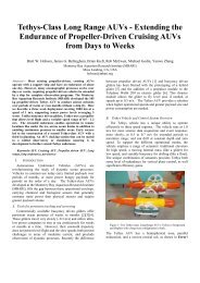
<strong>Continuous</strong> <strong>mission</strong> <strong>plan</strong> <strong>adaptation</strong> <strong>for</strong> <strong>autonomous</strong> <strong>vehicles</strong>:<br />
balancing ef<strong>for</strong>t and reward<br />
Pedro Patrón, David M. Lane, Yvan R. Petillot<br />
Ocean Systems Laboratory, Heriot-Watt University ∗<br />
EH14 4AS, Edinburgh, Scotland<br />
{p.patron,d.m.lane,y.r.petillot}@hw.ac.uk<br />
Abstract<br />
This paper proposes a novel approach <strong>for</strong> adaptive <strong>mission</strong><br />
<strong>plan</strong>ning <strong>for</strong> <strong>autonomous</strong> <strong>vehicles</strong> in a changing<br />
discoverable environment. The approach handles temporal<br />
<strong>plan</strong>ning with durative actions, metric <strong>plan</strong>ning,<br />
opportunistic <strong>plan</strong>ning and dynamic <strong>plan</strong>ning. During<br />
the <strong>plan</strong>ning process, <strong>plan</strong> selection is balanced between<br />
its estimated cost of execution and the reward<br />
obtained by reaching the new configuration of the environment.<br />
The <strong>plan</strong> proximity between <strong>plan</strong>s is defined<br />
in order to measure difference between <strong>plan</strong>s per<strong>for</strong>ming<br />
on the same execution environment. The approach<br />
is evaluated under a static scenario and a partially<br />
known dynamic scenario using the <strong>plan</strong> proximity to<br />
the human driven <strong>mission</strong>.<br />
Introduction<br />
Robotic plat<strong>for</strong>ms are helping humans to gain routine<br />
and permanent access to different environments. However,<br />
challenges related to difficult domains, such as<br />
underwater, require the integration of embedded tools<br />
that can raise the plat<strong>for</strong>m’s autonomy levels and adapt<br />
to the continuous changes on the perception that the<br />
plat<strong>for</strong>m has of the environment.<br />
The problem, however, is that at present, applications<br />
are mono-domain: <strong>mission</strong> targets are simply<br />
mono-plat<strong>for</strong>m, and <strong>mission</strong>s are generally static procedural<br />
lists of commands (Hagen 2001). If behaviours<br />
are added (Pang et al. 2003), they are only to cope with<br />
possible changes that are known a-priori by the operator.<br />
All this, there<strong>for</strong>e, leaves the plat<strong>for</strong>ms in isolation<br />
and limits the potential of adapting <strong>mission</strong> <strong>plan</strong>s to<br />
the sensing in<strong>for</strong>mation. The benefits of <strong>autonomous</strong><br />
dynamic <strong>mission</strong> <strong>plan</strong>ning in changing domains <strong>for</strong> has<br />
been promoted by Rajan et al. in (Rajan et al. 2007)<br />
and (McGann et al. 2007).<br />
We propose an approach based on a continuous reassessment<br />
of the status of the environment resources<br />
and the plat<strong>for</strong>m capabilities. The approach combines<br />
a Bayes model <strong>for</strong> prediction, measurement and correction<br />
(Thurn, Burgard, and Fox 2005) with the classical<br />
∗ This paper is partly funded by the Project<br />
RT/COM/5/059 from the Competition of Ideas and<br />
by the Project SEAS-DTC-AA-012 from the Systems<br />
Engineering <strong>for</strong> Autonomous Systems Defence Technology<br />
Centre, both established by the UK Ministry of Defence.<br />
<strong>plan</strong>ning approach. Instead of solving a <strong>plan</strong> from initial<br />
state to goals like in classical AI <strong>plan</strong>ning, the approach<br />
tries to maintain a window of actions that are<br />
believed can be per<strong>for</strong>med from of the current state in<br />
order to improve a given utility function.<br />
The paper is structured as follows: The following section<br />
describes the modeling of the environment of execution<br />
or domain. Next, we introduce the way the problem<br />
or <strong>mission</strong> gets represented. The proposed <strong>plan</strong><br />
strategy to solve this problem is described in the third<br />
section. A measure of <strong>plan</strong> proximity is proposed <strong>for</strong><br />
comparing different <strong>plan</strong>ning strategy results. Based on<br />
this metric, the final section analyses the per<strong>for</strong>mance<br />
of the approach in a static and in a partially known dynamic<br />
scenario. The paper ends with the conclusions<br />
and the future work.<br />
Domain Model<br />
We assume that the <strong>plan</strong>ner has access to the domain<br />
knowledge describing the list of actions/capabilities and<br />
resources.<br />
This domain is defined by the tuple Σ =<br />
(C, OC, VC, PV , AV ), where:<br />
• C = {ci|i ∈ 〈1, 2, . . . , |C|〉} 1 is a set of hierarchical<br />
classes of objects. All classes derive from a<br />
root class named object (e.g.: (:types location<br />
- object area - location ) class(c) represents<br />
the set <strong>for</strong>m by class c and all its ancestors:<br />
class(c) =<br />
{object}, if c=object<br />
{c} ∪ {class(parent(c))}, otherwise<br />
• OC = {o ci<br />
j |j ∈ 〈1, 2, . . . , |OC|〉, ci ∈ C} represents a<br />
set of objects or resources of C. Each object oj is of<br />
only one class ci. There<strong>for</strong>e each object oj belongs<br />
to its class and all the ancestors of this class (∀o ci<br />
j ∈<br />
OC class(oj) = class(ci)). (e.g.: seabedA - area<br />
indicates that the region ’seabedA’ belongs to the<br />
area, location and object classes).<br />
• VC = {v ci<br />
k |k ∈ 〈1, 2, . . . , |VC|〉, ci ∈ C} is a set<br />
of variables of C. In the same way, each variable<br />
vk belongs to its class and all the ancestors of this<br />
1 A set is a collection of elements. It is represented by {}.<br />
A list is an ordered set. It is represented by 〈〉.
class (∀v ci<br />
k ∈ VC class(vk) = class(ci)). (e.g.: ?v -<br />
vehicle indicates a variable v of the class vehicle).<br />
An ordered set of variables and objects defines a list<br />
of arguments <strong>for</strong> an item x:<br />
<br />
arg(x) = v ci<br />
k |k ∈ 〈1, 2, . . . , n〉,<br />
0 ≤ n ≤ |VC| + |OC|, ci ∈ C<br />
⊆ {VC ∪ OC}<br />
<br />
• PV = {pm|m ∈ 〈1, 2, · · · , |PV |〉} is a set of propositions.<br />
A proposition can return a boolean or a numeric<br />
value. Each proposition pm has a list of arguments<br />
arg(pm). (e.g.: (at ?l - location) represents<br />
the proposition of being at a particular location).<br />
FV = {fq, |q ∈ 〈1, 2, · · · , |FV |〉} ⊆ PV is a set of functions.<br />
A function is a proposition that returns a numeric<br />
value. (e.g.: (distance ?a ?b - location)<br />
represents the value of the distance between two locations).<br />
• AV = {ah, |h ∈ 〈1, 2, · · · , |AV |〉} is a set of<br />
actions. Each action ah has a list arguments<br />
arg(ah). An action can have a set of requirements:<br />
condition(ah) = {pm|pm ∈ PV ∧arg(pm) ⊆ arg(ah)}.<br />
An action can have a set of effects: effect(ah) =<br />
{pm|pm ∈ PV ∧ arg(pm) ⊆ arg(ah)}. An action<br />
has some duration in time: duration(ah) ∈ R.<br />
(e.g.: (move (?from ?to - location) (:dur<br />
(distance ?from ?to)) (:cond (at ?from))<br />
(:effect (not (at ?from)) (at ?to))).<br />
From this tuple, another two sets can be calculated:<br />
• RO = {rpm y |y ∈ 〈1, 2, · · · , |RO|〉, pm ∈<br />
PV , arg(rpm y ) ⊆ OC} is the set of proposition<br />
facts. A proposition fact rpm y is an instantiation of<br />
a proposition pm <strong>for</strong> a particular list of objects as<br />
arguments arg(rpm y ). (e.g.: (at seabedA)).<br />
• GO = {gah z |z ∈ 〈1, 2, · · · , |GO|〉, ah ∈ AV , arg(gah z ) ⊆<br />
OC} is the set of ground actions. A ground action<br />
gz is an instantiation of an action ah <strong>for</strong> a particular<br />
list of objects as arguments arg(rah z ). (e.g.: (move<br />
start seabedA)).<br />
An action can be probabilistic. Given an action ah<br />
with probabilistic effects, the uncertainty matrix Γ <strong>for</strong><br />
this action can be defined as:<br />
Γ(ah) |effect(ah)|×|RO| = {p(i|j)|<br />
i ∈ effect(ah), j ∈ RO}<br />
Problem Model<br />
t ∈ R defines the continuous time of the <strong>mission</strong>. s ∈<br />
N0 defines a discrete step or slot in time of a certain<br />
duration ds : [t s 0, t s n].<br />
A state at some particular step in time xs is a set containing<br />
in<strong>for</strong>mation of the available actions, available<br />
resources and the combination of possible proposition<br />
facts at that step:<br />
xs = xAV s ∪ xOC s ∪ xRO s<br />
= {i(x) ∈ [0; 1] ∀x ∈ {AV ∪ OC ∪ RO}}<br />
It can be seen that |xs| = |AV | + |OC| + |RO| .<br />
A ground action gah at step s defines a transition<br />
s<br />
function between states gah s : xs−1 → xs through the<br />
sequence of steps.<br />
A <strong>plan</strong> uT s defines a list of ground actions to<br />
be per<strong>for</strong>med in the T steps ahead uT s : xs−1 →<br />
〈gs, gs+1, · · · , gn|n ≤ T 〉, where T defines the number<br />
of ground actions (windows size) to be included in the<br />
continuous <strong>plan</strong>. T is also known as the <strong>plan</strong>ning horizon.<br />
et s defines the execution of gs at time t.<br />
Rewards<br />
Each object o ci<br />
j ∈ OC has a reward value δ(o ci<br />
j ).<br />
The reward of a proposition fact r pm<br />
y ∈ RO is the sum<br />
of all the rewards of the objects used as arguments:<br />
δ(r pm<br />
y ) = δ(o ci<br />
j )|∀oci j ∈ arg(rpm y )<br />
The reward of a state is the sum of all the rewards of<br />
the proposition facts available on it:<br />
δ(xs) = δ(r pm<br />
y )i(r pm<br />
y )|i(r pm<br />
y ) ∈ x RO<br />
s<br />
The set of <strong>mission</strong> goals can be defined explicitly with<br />
a list of rewards assigned to different proposition facts.<br />
• QO = {λ(rpm y )|rpm y<br />
∈ RO, arg(r pm<br />
y ) ⊆ OC} is the set<br />
of proposition fact goals. λ(r pm<br />
y ) is a reward defined<br />
by the operator. (e.g.: (= (surveyed seabedA)<br />
100)).<br />
The reward of a ground action g ah<br />
s is related to the<br />
production of a proposition fact that has been explicitly<br />
defined as a <strong>mission</strong> goal in the <strong>mission</strong> problem. This<br />
means that the ground action has to produce a goal<br />
proposition fact in the new state that was not available<br />
in the previous state:<br />
δ(g ah<br />
s , xs−1) = λ(r pm<br />
y )<br />
|rpm y ∈ {xRO s<br />
∧rpm y ∈ {xRO s<br />
∩ QO}<br />
∩ x RO<br />
s−1 }<br />
If ah has probabilistic effects, the reward of the<br />
ground action gah s is related to the probabilistic increase<br />
in the production of <strong>mission</strong> goals in the <strong>mission</strong> problem:<br />
δ(gah s , xs−1) = λ(rpm y )×<br />
(Γ(ah)[rpm |rpm y ∈ QO<br />
y |xs−1] − x RO<br />
s−1 [rpm y ])<br />
Costs<br />
Each ground action gah s has an execution cost when<br />
being executed in a state γ(gah s , xs−1).<br />
Payoffs<br />
The payoff function σ of a ground action gah s in a state<br />
xs−1 is the difference between its cost and the rewards<br />
of the proposition facts of the generated state xs:<br />
σ(g ah<br />
s , xs−1) = δ(xs)<br />
+δ(g ah<br />
s , xs−1)<br />
−γ(g ah<br />
s , xs−1)
The cumulative payoff of a <strong>plan</strong> us of length T given<br />
a state xs is the expected utility function of the <strong>plan</strong><br />
at that state σ(u T s , xs). It is the difference between the<br />
rewards accumulated through all the expected states<br />
and the ground actions in the <strong>plan</strong>:<br />
σ(u T s , xs−1) = E T <br />
τ=1<br />
β τ σ(g ah<br />
s+τ , xs+τ−1) <br />
where β ∈ [0; 1] is known as the discount factor. It<br />
represents the fact that actions that are <strong>plan</strong>ned in the<br />
long term may have less effect over the current state<br />
than short term actions.<br />
Passive Action<br />
An action should always exists called passive-action<br />
(φ). This action has no preconditions, no effects and a<br />
unitary cost (∀s, γ(g φ s , xs−1) = 1).<br />
Solution Approach<br />
The approach assumes that <strong>plan</strong>ning, observation and<br />
execution are per<strong>for</strong>med concurrently. Under such assumption,<br />
a <strong>plan</strong> is calculated up to a defined <strong>plan</strong>ning<br />
horizon. While executing this <strong>plan</strong>, the environment is<br />
continuously observed. When all the <strong>plan</strong> is executed,<br />
the <strong>plan</strong> is calculated. If the environment (resources<br />
and/or capabilities) changes, the approach supports a<br />
greedy and a lazy behaviour. Under the lazy behaviour,<br />
<strong>plan</strong>ning is only per<strong>for</strong>med at the end of the current<br />
<strong>plan</strong> execution ignoring changes on the environment.<br />
The greedy approach recalculates the <strong>plan</strong> as soon as<br />
the changes have being detected. The pseudo-code describing<br />
this process can be seen in Fig. 7.<br />
We assume a framework of stochastic environments<br />
with fully observable states. This is known as Markov<br />
decision processes. A policy in this framework is a mapping<br />
from states to <strong>plan</strong>s π : x → u. In this framework<br />
the current state is sufficient <strong>for</strong> determining the optimal<br />
control. A policy selects the <strong>plan</strong> u τ s of horizon<br />
τ that maximizes the expected cumulative payoff from<br />
the current state xs−1:<br />
π τ s (xs−1) = argmaxu [σ(u τ s, xs−1)] |1 ≤ τ ≤ T<br />
This policy is implemented using exhaustive <strong>plan</strong>ning<br />
search in the state-space. This policy is described in<br />
Fig. 8.<br />
Given a <strong>plan</strong> policy π τ s , the <strong>plan</strong> matrix ∆ τ s contains<br />
in<strong>for</strong>mation of the expected actions and resources used<br />
by the <strong>plan</strong> ahead. This matrix has T rows and |AV | +<br />
|OC| columns:<br />
∆ τ s = [µ] T ×|AV |+|OC||µ ∈ [0; 1]<br />
Given a row ς ≤ τ and an action ah,<br />
µς,ah =<br />
1, if gs+ς ∈ π τ s (xs−1)<br />
0, otherwise<br />
Given a row ς and an object oj,<br />
µς,oj =<br />
Action Management<br />
1, if oj ∈ xs+ς<br />
0, otherwise<br />
• Removal of an action that is not in <strong>plan</strong>: In this case<br />
the state is corrected and the execution continues.<br />
• Removal of an action that is in the <strong>plan</strong>: In this case<br />
the state and the <strong>plan</strong> are corrected.<br />
• Action recovery: In this case, an action/capability<br />
that was previously available is recovered. The state<br />
gets corrected, and the <strong>plan</strong> is not guaranteed to be<br />
optimal <strong>for</strong> the window if a lazy approach is used. A<br />
lazy approach means that the <strong>plan</strong> only gets recalculated<br />
when the <strong>plan</strong> is empty.<br />
• New action: When a new action is inserted in the<br />
system, the state and <strong>plan</strong> need to be corrected.<br />
Object Management<br />
• Removal of an object that is part of the current state:<br />
In this case the framework becomes unstable as the<br />
system no longer has available an object that was<br />
being used.<br />
• Removal of an object used in the <strong>plan</strong>: In this case,<br />
the states needs to get corrected and the <strong>plan</strong> recalculated.<br />
• Other removal of objects: In this case, only the state<br />
needs correction.<br />
• Object recovery: In a similar way as <strong>for</strong> the action<br />
recovery, when an object that was not available previously<br />
is recovered the state needs to get corrected.<br />
The <strong>plan</strong> is not guaranteed to be optimal <strong>for</strong> the window<br />
if a lazy approach is used.<br />
• New object: When a new object is added, the state<br />
and the <strong>plan</strong> need to be corrected.<br />
Predicate Management or Explicit Goals<br />
Predicates can be managed through the use of goals.<br />
Goals are predicate facts that the operator want them<br />
to happen.<br />
Action with Probabilistic Effects<br />
Actions can have probabilistic effects. In this case, the<br />
in<strong>for</strong>mation of the state vector is probabilistic. The<br />
reward of the proposition facts in the goals is affected<br />
by the probabilistic effect of the actions.<br />
In<strong>for</strong>mation Exchange<br />
It can be seen that in<strong>for</strong>mation about the current availability<br />
of actions and resources is stored in a single<br />
binary state vector. This vector can be easily compressed<br />
and transfered using low bandwidth communication<br />
hardware such as acoustic modems.
Plan Proximity<br />
Plan proximity measures the similarity between two<br />
<strong>plan</strong>s. Plan proximity can be calculated from the<br />
<strong>plan</strong> difference and the state difference of the outcome<br />
states (Patrón and Birch 2009).<br />
The <strong>plan</strong> difference between u1 and u2, Dp(u1, u2) is<br />
the number of missing actions mp from the reference<br />
<strong>plan</strong> u1 and the number of extra actions ep from a test<br />
<strong>plan</strong> u2 that do not appear in the longest common subsequence<br />
of actions (Hunt and McIlroy 1976). The <strong>plan</strong><br />
difference is normalized using the sum of the number of<br />
actions of the reference <strong>plan</strong> n1 and the test <strong>plan</strong> n2.<br />
ˆDp(u1, u2) = mp + ep<br />
∈ [0; 1]<br />
n1 + n2<br />
The state difference can be calculated as the Hamming<br />
distance (Hamming 1950) between the string representation<br />
of s1 and s2. The state difference is normalized<br />
using the string length m.<br />
ˆDs(s1, s2) =<br />
m<br />
i=1 xi<br />
m<br />
where xi =<br />
0 if s1(i) = s2(i)<br />
1 otherwise<br />
Plan proximity, P P (u1, u2), is defined as the normalized<br />
balanced sum of the <strong>plan</strong> difference Dp(u1, u2) and<br />
the state difference of the estimated final states that<br />
they are expected to produce Ds(G1, G2).<br />
P Pα(u1, u2) = 1 −α · ˆ Dp(u1, u2)<br />
−(1 − α) · ˆ Ds(G1, G2) ∈ [0; 1]<br />
where α ∈ [0; 1] represents a balance factor between<br />
<strong>plan</strong> and state difference.<br />
Plan proximity is more in<strong>for</strong>med than <strong>plan</strong> stability<br />
(Fox et al. 2006) <strong>for</strong> measuring <strong>plan</strong> strategies solving<br />
the dynamic <strong>plan</strong>ning problem as it takes into account<br />
actions missing from the reference <strong>plan</strong>, extra actions<br />
added in the test <strong>plan</strong>, sequential ordering of the<br />
<strong>plan</strong>s and the expected outcomes states of these <strong>plan</strong>s.<br />
Evaluation<br />
Using this metric, the approach has been evaluated under<br />
the scenario described by the Student Autonomous<br />
Underwater Challenge - Europe <strong>mission</strong> rules (SAUC-<br />
E 2009). For this competition the scenario is <strong>for</strong>m by<br />
three aligned gates, a bottom target, a moving midwater<br />
target, two wall sections and a docking station.<br />
The vehicle should pass through three aligned gates,<br />
first <strong>for</strong>ward and then backwards. Green and red lights<br />
on the second gate indicate the route that should be<br />
taken <strong>for</strong> its avoidance during the <strong>for</strong>ward pass. After<br />
passing the gates in and out, the vehicle should attempt<br />
(in no particular order) to per<strong>for</strong>m an inspection of the<br />
bottom target, to follow the moving mid-water target,<br />
to survey the walls and to dock at the docking station.<br />
The scenario is represented in Fig. 1.<br />
The scenario is described using four files based on the<br />
PDDL syntax (Ghallab et al. 1998):<br />
Position and orientation of objects other than<br />
the gates are given as an example. They could<br />
be changed daily.<br />
Mid column moving target<br />
Validation Gate<br />
Hovering target<br />
Gate 2<br />
Reference Frame z downward<br />
Gate 3<br />
Wall to be survey<br />
Docking box<br />
Figure 1 :Mission Illustration<br />
Figure 1: Scenario of the 2009 Student Autonomous<br />
Underwater Challenge - Europe. Mission starting at<br />
the origin. Gates, bottom target, mid-water target, wall<br />
sections and docking station locations are shown.<br />
NOTES:<br />
! Submerge and the validation gate MUST be undertaken first. The other tasks may be<br />
undertaken in any order.<br />
! Tasks may be attempted individually from a start point requested by teams. Points<br />
can be collected <strong>for</strong> the successful completion of tasks throughout the practice days,<br />
qualification and final 6 .<br />
! For completing all the tasks in a single joined up <strong>mission</strong>, extra points will be<br />
awarded, See scoring section.<br />
! Between subsequent entry runs the in-water targets may be moved in position and/or<br />
depth.<br />
! The vehicle MUST remain fully submerged. Surfacing at any time will result in<br />
termination of that <strong>mission</strong>.<br />
! The use of a Doppler Velocity Log will be strictly prohibited 7 of OC, the predicates PV , the functions FV and the<br />
actions AV .<br />
.<br />
• The domain: describes the classes in C, constants<br />
• The problem: describes the initial state x0, the rewards<br />
δ(OC), the goals QO and the cost metric γ.<br />
6<br />
Points <strong>for</strong> completing an individual task will only be awarded once <strong>for</strong> that task.<br />
• 7 The This expensive world commercial model: equipment describes would give an unfair theadvantage known to the objects cash rich teams, inwithout OC<br />
contributing and their to the advancement particular of the vehicle’s domain autonomy. properties. These properties<br />
allow the calculation of the functions in FV .<br />
• The dynamic world model: simulates events that occur<br />
on the execution time line. Events can be triggered<br />
by a predicate in the current state or by reaching<br />
a slot. They can add, delete and restore objects,<br />
actions and predicates from the current knowledge.<br />
Known Static Environment<br />
This section analyses the outcomes of the proposed<br />
<strong>plan</strong>ning strategies in a fully known static environment.<br />
In this case, the world model contains all the in<strong>for</strong>mation<br />
about the environment and the dynamic world file<br />
is empty.<br />
The different <strong>plan</strong>ning strategies are evaluated looking<br />
at their <strong>plan</strong> proximity to u0 (see Fig.2) after removing<br />
any instances of the passive action φ that may<br />
appear on the <strong>plan</strong>. Each approach was executed until<br />
t > 220 seconds. Fig.3 describes the cumulative<br />
payoff <strong>for</strong> different <strong>plan</strong>ning strategies. Table 1 shows<br />
<strong>plan</strong> proximity to u0 of different <strong>plan</strong>ning strategies.<br />
T ∈ 2, 3, 4 generates the same <strong>plan</strong> as the human. T = 1<br />
does not have enough evidence about rewards to commit<br />
to different actions other than the passive action.<br />
T = 5 reaches the exhaustive search limits and stops a<br />
step be<strong>for</strong>e providing the final section of the <strong>plan</strong>.<br />
Partially-known Dynamic Environment<br />
This section analyses the outcomes of the proposed<br />
<strong>plan</strong>ning strategies when solving the dynamic <strong>plan</strong>ning<br />
problem under the same scenario. In this case, the original<br />
world model only contains in<strong>for</strong>mation about the<br />
x<br />
y
ight<br />
centre<br />
down<br />
red<br />
off<br />
recovery<br />
middle<br />
wall1<br />
wall2<br />
<strong>for</strong>ward<br />
bottom<br />
downward<br />
up<br />
gate3<br />
gate2<br />
gate1<br />
lstart<br />
toWait<br />
toDock<br />
toFollow<br />
toSurvey<br />
toInspect<br />
toTraverse−out<br />
toTurn<br />
toTraverse−in<br />
toMove<br />
●<br />
●<br />
●<br />
●<br />
●<br />
●<br />
●<br />
●●<br />
●<br />
●<br />
●<br />
●●<br />
●<br />
●<br />
●<br />
●<br />
●<br />
●<br />
●<br />
● ● ●●<br />
●<br />
●<br />
●<br />
●<br />
●●<br />
●<br />
●<br />
●<br />
●●<br />
●<br />
● ●<br />
●<br />
●<br />
●<br />
●<br />
●<br />
●<br />
●<br />
●<br />
action<br />
arg1<br />
arg2<br />
arg3<br />
● ●<br />
0 50 100 150 200<br />
●<br />
●<br />
Time(s)<br />
●<br />
●<br />
● ●<br />
Figure 2: Ground actions with their arguments executed<br />
over time during the human generated <strong>plan</strong> u0.<br />
This <strong>plan</strong> is used as ground truth <strong>for</strong> the evaluation of<br />
the different <strong>plan</strong>ning strategies.<br />
T Dp<br />
ˆ ˆDs P P0.5<br />
1 1.00 0.21 0.39<br />
2 0.00 0.00 1.00<br />
3 0.00 0.00 1.00<br />
4 0.00 0.00 1.00<br />
5 0.21 0.04 0.87<br />
Table 1: Plan proximity to u0 <strong>for</strong> the approaches using<br />
T ∈ [1; 5] in the known static environment.<br />
first gate and the docking station. The dynamic world<br />
model file simulates a series of events that add, delete<br />
or restore objects and/or actions on the world model.<br />
Fig.4 shows the evolution of capabilities and resources<br />
over time <strong>for</strong> the case of the human driven <strong>mission</strong>.<br />
Fig. 5 represents the human driven <strong>mission</strong> as it was<br />
adapted by the human to cope with the changes perceived<br />
in the environment by the world model. It can<br />
be seen how the operator is <strong>for</strong>ced to insert a series of<br />
passive action instances as the action toWait becomes<br />
unavailable until s = 22 while being at gate2. Table 2<br />
represents the <strong>plan</strong> proximity to u0 of the different <strong>plan</strong>ning<br />
strategies solving the dynamic <strong>plan</strong>ning problem<br />
scenario. It can be seen that the <strong>plan</strong>ning strategy solutions<br />
<strong>for</strong> T ∈ 3, 4, 5 are as close to u0 as the human.<br />
Conclusion<br />
We have presented an approach <strong>for</strong> continuous <strong>mission</strong><br />
<strong>plan</strong>ning <strong>for</strong> <strong>autonomous</strong> <strong>vehicles</strong>. The approach handles<br />
temporal <strong>plan</strong>ning with durative actions, metric<br />
<strong>plan</strong>ning, opportunistic <strong>plan</strong>ning and dynamic <strong>plan</strong>ning.<br />
During the <strong>plan</strong>ning process, the action selec-<br />
●<br />
●<br />
●<br />
●<br />
●<br />
●<br />
●<br />
●<br />
● ●<br />
●<br />
●<br />
●<br />
●<br />
Cumulative Payoff<br />
1000<br />
800<br />
600<br />
400<br />
200<br />
0<br />
0.9<br />
5<br />
1<br />
5<br />
0 50 100 200<br />
0 50 100 200<br />
0.9<br />
4<br />
1<br />
4<br />
0.9<br />
3<br />
1<br />
3<br />
0 50 100 200<br />
Time (s)<br />
Greedy Lazy<br />
0 50 100 200<br />
0.9<br />
2<br />
1<br />
2<br />
1<br />
1<br />
0 50 100 200<br />
Figure 3: Cumulative payoff of different <strong>plan</strong>ning strategy<br />
results solving the known static scenario. T ∈ [1; 5],<br />
β ∈ [0.9; 1] and lazy ∈ [0; 1].<br />
T Dp<br />
ˆ ˆDs P P0.5<br />
H 0.18 0.01 0.90<br />
1 1.00 0.25 0.37<br />
2 0.41 0.06 0.76<br />
3 0.15 0.01 0.91<br />
4 0.20 0.01 0.89<br />
5 0.20 0.01 0.89<br />
Table 2: Plan proximity to u0 <strong>for</strong> the different <strong>plan</strong>ning<br />
strategies using the human H and T ∈ [1; 5] in a<br />
partially-known dynamic environment.<br />
tion is balanced between its estimated cost of execution<br />
and the reward obtained by reaching the new configuration<br />
of the environment. A <strong>plan</strong> proximity metric<br />
has been defined in order measure difference between<br />
<strong>plan</strong>s per<strong>for</strong>ming on the same execution environment.<br />
The approach is evaluated under a static scenario and<br />
a partially known dynamic scenario showing that the<br />
results are close to the ones provided by the human.<br />
In the future we are going to be looking at the limitations<br />
of the <strong>plan</strong>ning horizon, more in<strong>for</strong>med policies,<br />
and the discovery of actions and resources via a serviceoriented<br />
architecture.<br />
References<br />
Fox, M.; Gerevini, A.; Long, D.; and Serina, I. 2006.<br />
Plan stability: Re<strong>plan</strong>ning versus <strong>plan</strong> repair. In Int.<br />
Conf. on Automated Planning and Scheduling.<br />
Ghallab, M.; Howe, A.; Knoblock, C.; McDermott,<br />
D.; Ram, A.; Veloso, M.; Weld, D.; and Wilkins, D.<br />
1998. Pddl: The <strong>plan</strong>ning domain definition language.<br />
0.9<br />
1<br />
1000<br />
800<br />
600<br />
400<br />
200<br />
0
Capability<br />
Resource<br />
toDock<br />
toFollow<br />
toInspect<br />
toSurvey<br />
toTurn<br />
toTraverse−out<br />
toTraverse−in<br />
toMove<br />
toWait<br />
green<br />
red<br />
video<br />
sidescan<br />
<strong>for</strong>ward<br />
downward<br />
recovery<br />
lstart<br />
gate1<br />
off<br />
wall2<br />
wall1<br />
middle<br />
bottom<br />
gate3<br />
gate2<br />
detached<br />
engaged<br />
centre<br />
right<br />
left<br />
down<br />
up<br />
0<br />
1<br />
2<br />
3<br />
4<br />
5<br />
6<br />
7<br />
8<br />
9<br />
10<br />
11<br />
12<br />
13<br />
14<br />
15<br />
16<br />
17<br />
18<br />
19<br />
20<br />
21<br />
22<br />
23<br />
24<br />
25<br />
26<br />
27<br />
28<br />
29<br />
30<br />
31<br />
32<br />
33<br />
34<br />
35<br />
36<br />
37<br />
38<br />
39<br />
40<br />
41<br />
Slot<br />
0<br />
1<br />
2<br />
3<br />
4<br />
5<br />
6<br />
7<br />
8<br />
9<br />
10<br />
11<br />
12<br />
13<br />
14<br />
15<br />
16<br />
17<br />
18<br />
19<br />
20<br />
21<br />
22<br />
23<br />
24<br />
25<br />
26<br />
27<br />
28<br />
29<br />
30<br />
31<br />
32<br />
33<br />
34<br />
35<br />
36<br />
37<br />
38<br />
39<br />
40<br />
41<br />
Figure 4: Evolution of capabilities and resources over<br />
time <strong>for</strong> the human driven <strong>mission</strong> (dark grey means unavailable).<br />
gate2, gate3, bottom, middle, wall1 and<br />
wall2 are discovered during the <strong>mission</strong>. gate2 lights<br />
are discovered and change colour during the <strong>mission</strong>.<br />
<strong>for</strong>ward camera and action toMove are temporarily unavailable<br />
during the <strong>mission</strong>.<br />
right<br />
centre<br />
red<br />
off<br />
recovery<br />
middle<br />
wall1<br />
wall2<br />
<strong>for</strong>ward<br />
bottom<br />
downward<br />
gate3<br />
down<br />
up<br />
gate2<br />
gate1<br />
lstart<br />
toDock<br />
toFollow<br />
toSurvey<br />
toInspect<br />
toWait<br />
toTraverse−out<br />
toTurn<br />
toTraverse−in<br />
toMove<br />
●<br />
●<br />
●<br />
●<br />
●<br />
●●<br />
●<br />
●<br />
●<br />
●<br />
●<br />
●<br />
●<br />
● ● ●<br />
●<br />
●<br />
●<br />
●<br />
●<br />
● ●●<br />
● ●<br />
● ●<br />
● ●<br />
●<br />
●<br />
●<br />
●<br />
● ● ●<br />
●●<br />
●<br />
●<br />
●<br />
●<br />
action<br />
arg1<br />
arg2<br />
arg3<br />
●<br />
●<br />
●<br />
Time(s)<br />
Slot<br />
0 50 100 150 200<br />
●<br />
●<br />
●<br />
●<br />
● ● ●<br />
Figure 5: Ground actions with their arguments executed<br />
over time <strong>for</strong> the human driven <strong>mission</strong> in the<br />
dynamic environment scenario.<br />
Technical report, Yale Center <strong>for</strong> Computational Vision<br />
and Control.<br />
Hagen, P. 2001. Auv/uuv <strong>mission</strong> <strong>plan</strong>ning and real<br />
time control with the hugin operator system. In IEEE<br />
OCEANS 2001, volume 1, 468–473.<br />
●<br />
●<br />
●<br />
●<br />
●<br />
● ●<br />
●<br />
●<br />
●<br />
●<br />
● ●<br />
●<br />
●<br />
●<br />
Cumulative Payoff<br />
1000<br />
500<br />
0<br />
0.9<br />
5<br />
1<br />
5<br />
0 50 100 200<br />
0 50 100 200<br />
0.9<br />
4<br />
1<br />
4<br />
0.9<br />
3<br />
1<br />
3<br />
0 50 100 200<br />
Time (s)<br />
Greedy Lazy<br />
0 50 100 200<br />
0.9<br />
2<br />
1<br />
2<br />
1<br />
1<br />
0 50 100 200<br />
Figure 6: Cumulative payoff of different <strong>plan</strong>ning strategy<br />
results solving the partially known dynamic scenario.<br />
T ∈ [1; 5], β ∈ [0.9; 1] and lazy ∈ [0; 1].<br />
Hamming, R. W. 1950. Error detecting and error<br />
correcting codes. Bell System Technical Journal 29<br />
2:147–160.<br />
Hunt, J. W., and McIlroy, M. D. 1976. An algorithm<br />
<strong>for</strong> differential file comparison. Computing Science<br />
Technical Report, Bell Laboratories 41.<br />
McGann, C.; Py, F.; Rajan, K.; Thomas, H.; Henthorn,<br />
R.; and McEwen, R. 2007. T-rex: A modelbased<br />
architecture <strong>for</strong> auv control. In Workshop in<br />
Planning and Plan Execution <strong>for</strong> Real-World Systems:<br />
Principles and Practices <strong>for</strong> Planning in Execution,<br />
International Conference of Autonomous Planning<br />
and Scheduling.<br />
Pang, S.; Farrell, J.; Arrieta, R.; and Li, W. 2003. Auv<br />
reactive <strong>plan</strong>ning: deepest point. In IEEE OCEANS<br />
2003, volume 4, 2222–2226.<br />
Patrón, P., and Birch, A. 2009. Plan proximity: an<br />
enhanced metric <strong>for</strong> <strong>plan</strong> stability. In Workshop on<br />
Verification and Validation of Planning and Scheduling<br />
Systems, 19th International Conference on Automated<br />
Planning and Scheduling.<br />
Rajan, K.; McGann, C.; Py, F.; and Thomas, H.<br />
2007. Robust <strong>mission</strong> <strong>plan</strong>ning using deliberative autonomy<br />
<strong>for</strong> <strong>autonomous</strong> underwater <strong>vehicles</strong>. In ICRA<br />
Robotics in challenging and hazardous environments.<br />
SAUCE. 2009. Mission rules <strong>for</strong> the student <strong>autonomous</strong><br />
underwater challenge 2009 - europe v.1.<br />
Technical report, Defence Science and Technology<br />
Laboratory - Ministry of Defence, UK.<br />
Thurn, S.; Burgard, W.; and Fox, D. 2005. Probabilistic<br />
robotics. MIT Press.<br />
0.9<br />
1<br />
1000<br />
500<br />
0
t ← s ← 0<br />
T ← τ ← <strong>plan</strong>ning horizon<br />
xs ← xAV s ∪ xOC s ∪ xRO s<br />
greedy ← TRUE ∨ FALSE<br />
∆ τ s ← zeroT ×|AV |+|OC|<br />
s ← s + 1<br />
<strong>for</strong>ever do<br />
;; <strong>adaptation</strong><br />
τ ← T<br />
(πτ s , ∆τ s) ← argmaxu [σ(uτ s, xs−1)]<br />
recalculate ← FALSE<br />
while (recalculate = TRUE) do<br />
;; execute first action in the <strong>plan</strong><br />
et s ← g0(πτ s ))<br />
;; predict next state<br />
(xs+1, ∆ τ−1<br />
s+1 ) ← exec(ets) ;; observe state<br />
x ′ s+1 ← world model<br />
;; diagnosis<br />
if (|xs+1| < |x ′ s+1|)<br />
recalculate ← TRUE<br />
else<br />
if (xs+1 ⊃ x ′ s+1) ∧ ( ∆ τ−1<br />
s+1 x′AV s+1 ∪ x′OC s+1 |∀ς ≤ τ − 1) then<br />
if ( ∆ τ−1<br />
s+1 (ets) x ′AV<br />
s+1 ∪ x′OC s+1 ) then<br />
unstable, execute emergency script!!!<br />
endif<br />
recalculate ← TRUE<br />
endif<br />
if (xs+1 ⊂ x ′ s+1) ∧ ( ∆ τ−1<br />
s+1 ⊆ x′AV s+1 ∪ x′OC s+1 |∀ς ≤ τ − 1) ∧ (greedy) then<br />
recalculate ← TRUE<br />
endif<br />
endif<br />
;; correction<br />
xs+1 ← x ′ s+1<br />
t ← t + duration(et s)<br />
τ ← τ − 1<br />
s ← s + 1<br />
if (τ = 0) then<br />
recalculate ← TRUE<br />
endif<br />
endwhile<br />
end<strong>for</strong><br />
Figure 7: Approach in Pseudo-code
function SearchPolicy(xs, T )<br />
;; initialize policy to the laziest <strong>plan</strong>: a sequence of pasive actions<br />
π T s ← {φ1, φ2, · · · , φT }<br />
σ(π T s , xs) ← goals(xs) + T × δ(xs)<br />
∆ T s ← zero T ×|AV |+|OC|<br />
;; initialize search variables<br />
τ ← 0<br />
µ τ s ← {}<br />
σ(µ τ s, xs) ← 0<br />
∆ τ s ← zero T ×|AV |+|OC|<br />
;; launch exhaustive search<br />
ExhaustiveSearch(π T s , σ(π T s , xs), ∆ T s , xs, τ, µ τ s, σ(µ τ s, xs), ∆ τ s )<br />
return (π T s , σ(π T s , xs), ∆ T s )<br />
endfunction<br />
function ExhaustiveSearch(π T s , σ(π T s , xs), ∆ T s , xs+τ , τ, µ τ s, σ(µ τ s, xs)), ∆ τ s)<br />
;; if the <strong>plan</strong>ning horizon is reached<br />
if (τ = T ) then<br />
;; if the <strong>plan</strong> found is better than the current one<br />
if (σ(µ τ , xs) > σ(π T s , xs)) then<br />
;; adopt new <strong>plan</strong><br />
π T s ← µ T s<br />
σ(π T s , xs) ← σ(µ τ , xs)<br />
∆ T s ← ∆ τ s<br />
endif<br />
return<br />
endif<br />
τ ← τ + 1<br />
Uτ ← {gs+τ ∈ GO ∧ executable(xs+τ−1)}<br />
;; <strong>for</strong> each of the ground action candidates<br />
<strong>for</strong>each (es+τ ∈ Uτ ) do<br />
Uτ ← Uτ \ es+τ<br />
(xs+τ , ∆ τ s) ← execute(es+τ , xs+τ−1)<br />
µ T s ← µ T s ∪ {es+τ }<br />
σ(µ T , xs) ← σ(µ T , xs) + β τ σ(es+τ , xs+τ−1)<br />
ExhaustiveSearch(π T s , σ(π T s , xs), ∆ T s , xs+τ , τ, µ τ s, σ(µ τ , xs), ∆ τ s)<br />
µ T s ← µ T s \ {es+τ }<br />
σ(µ T , xs) ← σ(µ T , xs) − β τ σ(es+τ , xs+τ−1)<br />
end<strong>for</strong><br />
return (π T s , σ(π T s , xs), ∆ T s )<br />
endfunction<br />
Figure 8: Search process <strong>for</strong> the optimal policy in Pseudo-code