waders and their estuarine food supplies - Vlaams Instituut voor de ...
waders and their estuarine food supplies - Vlaams Instituut voor de ...
waders and their estuarine food supplies - Vlaams Instituut voor de ...

Create successful ePaper yourself
Turn your PDF publications into a flip-book with our unique Google optimized e-Paper software.
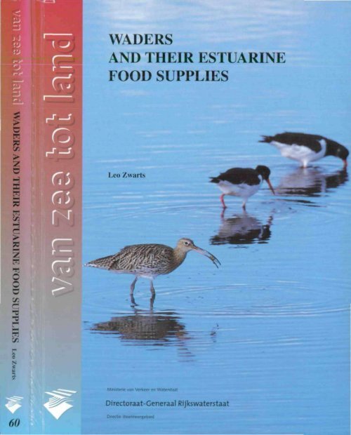
WADERS<br />
AND THEIR ESTUARINE<br />
FOOD SUPPLIES<br />
Len /warts<br />
••'ne van Ven<br />
Directoraat-Generaal Rijkswaterstaat<br />
..ubied
1. Schol helpt scholekster.<br />
STELLINGEN<br />
behoren<strong>de</strong> bij het proefschrift<br />
Wa<strong>de</strong>rs <strong>and</strong> <strong>their</strong> <strong>estuarine</strong> <strong>food</strong> <strong>supplies</strong><br />
van Leo Zwarts<br />
2. Aangezien <strong>de</strong> variatie in het daadwerkelijke voedselaanbod veelal meer<br />
wordt bepaald door <strong>de</strong> enorme variatie in <strong>de</strong> OOgStbare fractie van het voed<br />
sel dan door <strong>de</strong> variatie in het totale hoeveelheid voedsel. is het altijd lonend<br />
om bij on<strong>de</strong>rzoek naar predator-prooi-relaties <strong>de</strong> bereikbaarheid van het<br />
voedsel en <strong>de</strong> prooiselectie van <strong>de</strong> predator nauwkeurig te kwantificeren.<br />
3. Als dominante vogels min<strong>de</strong>r lichaarasreserves aanleggen dan suhdominan-<br />
te vogels. is dit niet omdat het dominant zijn zoveel energie kost. maar omdat<br />
vogels die hoog in <strong>de</strong> pikor<strong>de</strong> staan kennelijk met een kleinere energetische<br />
nood<strong>voor</strong>raad <strong>de</strong>nken te kunnen volstaan (contra J.M. Bowler (1994) Ar<strong>de</strong>a<br />
82: 241-248).<br />
4. De sterfte die optreedt bij het vangen van vogels met behulp van netten ten<br />
behoeve van wetenschappelijk on<strong>de</strong>rzoek uon.lt len onrechte nooit on<strong>de</strong>r<br />
worpen aan een kritische evaluatie. Zeker wanneer hel on<strong>de</strong>rzoek afhankelijk<br />
is van <strong>de</strong> terugvangst van individuele vogels moet <strong>de</strong>ze mortaliteit wor<strong>de</strong>n<br />
geschat.
plia^ohi. <br />
WADERS AND THEIR ESTUARINE FOOD SUPPLIES<br />
UITNODIGING<br />
lot het bijwonen van <strong>de</strong> ver<strong>de</strong>diging van het proefschrift<br />
en <strong>de</strong> daarbij behoren<strong>de</strong> stellingen op<br />
vrijdag 10 januari 1997 om vier tun preeies<br />
in het Aca<strong>de</strong>mie-gebouw. Broerstraat 5. Groningen<br />
Na afloop reeeptie in het Aca<strong>de</strong>mie-gebouw<br />
Leo Zwarts<br />
huidig adres:<br />
werk: RIZA<br />
Postbus 17<br />
8200 AA Lelystad<br />
of prise:<br />
Compagnonsweg 45/47<br />
8427 RH Ravenswoud<br />
tei. 0516-433905
5. Aangezien vele van <strong>de</strong> wei<strong>de</strong>- en moerasvogels die hier te l<strong>and</strong>e broe<strong>de</strong>n. het<br />
grootste <strong>de</strong>el van het jaar geeonecntreerd zijn in Afrikaanse moerasgebie<strong>de</strong>n,<br />
is <strong>de</strong> toekomst van <strong>de</strong>ze vogels in sterke mate afhankelijk van <strong>de</strong> gang van<br />
zaken in <strong>de</strong>ze overwinteringsgebic<strong>de</strong>n.<br />
6. Jaeht heeft een negatieve effect op <strong>de</strong> omvang van een dierpopulatie omdat.<br />
als gevolg van <strong>de</strong> toename in <strong>de</strong> schuwheid van <strong>de</strong> bejaag<strong>de</strong> dieren. het<br />
gebruik van hun leefgebied wordt beperkt. Dit indirecte effect iv waarschijn<br />
lijk van veel groter belang dan het direct meetbare effect van <strong>de</strong> verhoog<strong>de</strong><br />
mortaliteil als gevolg van het afschot.<br />
7. Mensen die in <strong>de</strong> tropen leven, crvarcn <strong>de</strong> natuur veelal als een bron van<br />
gc\aren en zel<strong>de</strong>n als een plek waar het aangenaam verpozen is. Dit bemoei-<br />
lijkt <strong>de</strong> export van <strong>de</strong> natuurbeschermingsgedachte vanuit <strong>de</strong> gematig<strong>de</strong> stre-<br />
ken naar <strong>de</strong> tropen.<br />
8. Het feit dat <strong>de</strong> meeste. /ells duur uitgevoer<strong>de</strong>. rapporten wor<strong>de</strong>n uitgebraeht<br />
zon<strong>de</strong>r dat titel en auteur op <strong>de</strong> rug wor<strong>de</strong>n vermeld, doet vermoe<strong>de</strong>n dat het<br />
<strong>de</strong> bedoeling is ze te bewaren in een bureaula en niet in een boekenkast.
Wa<strong>de</strong>rs <strong>and</strong> <strong>their</strong> <strong>estuarine</strong> <strong>food</strong> <strong>supplies</strong>
Ministerie van Verkeer en Waterstaat<br />
Directoraai-Generaal Rijkswaterstaat<br />
I)iredic IJsse 1 meergebied<br />
Van Zee tot L<strong>and</strong> 60<br />
Lelystad 1996<br />
ISBN 90-369-1183-4
WADERS AND THEIR ESTUARINE<br />
FOOD SUPPLIES<br />
Leo Zwarts<br />
Van Zee tot L<strong>and</strong> 60
Dil rapport vorm<strong>de</strong> tevens het proefschrift waarop <strong>de</strong><br />
auteur op 10 januari 1997 pnnnoveer<strong>de</strong> aan <strong>de</strong><br />
Rijksuniversiteil te Groningen.<br />
Als promotor trad op prof. dr. KH. Drent
figuren: Dick Visser<br />
omslagfoto: Jan van <strong>de</strong> Kant<br />
lulu's \un l<strong>and</strong>schappen, bo<strong>de</strong>mdieren en vogels: Jan van tic Kam<br />
overige loin's: Jan H. Wanink en Leo Zwarts<br />
vogeltekeningen: Jos Zwarts<br />
DTP en drukwerh Evers Litho & Druk<br />
codrdinatie productie: Henk Bos
CONTENTS<br />
Introduction 9<br />
1 Seasonal variation in body weight of the bivalves Macoma halihica. Scrobicularia plana,<br />
Mya arenaria <strong>and</strong> Cerasto<strong>de</strong>ma edule in the Dutch Wad<strong>de</strong>n Sea 25<br />
2 How the <strong>food</strong> supply harvestable by <strong>wa<strong>de</strong>rs</strong> in the Wad<strong>de</strong>n Sea <strong>de</strong>pends on the variation in energy<br />
<strong>de</strong>nsity, body weight, biomass. burying <strong>de</strong>pth <strong>and</strong> behaviour of tidal-flat invertebrates. 45<br />
3 Burying <strong>de</strong>pth of the benthic bivalve Scrobicularia plana (da Costa) in relation to<br />
siphon-cropping. 83<br />
4 Siphon si/e <strong>and</strong> burying <strong>de</strong>pth in <strong>de</strong>posit- <strong>and</strong> suspension-feeding benthic bivalves. 95<br />
5 Feeding radius, burying <strong>de</strong>pth <strong>and</strong> siphon length of Macoma halthica <strong>and</strong> Scnibicularia plana. 111<br />
6 The maerobenlhos fraction accessible to <strong>wa<strong>de</strong>rs</strong> often represents marginal prey. 127<br />
7 Doev an optimally foraging oystercatcher obey the functional response' 137<br />
8 Prey size selection <strong>and</strong> intake rate. 153<br />
9 Causes nl variation in prey profitability <strong>and</strong> its consequences lor the intake rate of 0\ stercatehers<br />
llticnuiiopiis oslralegus. 173<br />
10 Why Oystercatcher Haeinatopiis nstralegus cannot meet <strong>their</strong> daily energy requirements in a<br />
single low water period. 211<br />
11 Predicting seasonal <strong>and</strong> annual fluctuations in the local exploition of different prey by<br />
()\ steicatcher Haematopus oslralegus: a ten year study in the Wad<strong>de</strong>n Sea. 231<br />
12 Why knot Calklris eanutus take medium-sized Macoma bnliltica when six prey species are<br />
available. 267<br />
13 Annual <strong>and</strong> seasonal variation in the <strong>food</strong> supply harvestable by knot Calidrii caiuittis staging in the<br />
Wad<strong>de</strong>n Sea in late summer. 287<br />
14 Seasonal trend in burrow <strong>de</strong>pth <strong>and</strong> tidal variation in surface feeding of Xereis diverslcolor. 301
15 Versatility of male curlews (Numenius arquata) preying upon Nereis diversicolor: <strong>de</strong>ploying<br />
contrasting capture mo<strong>de</strong> <strong>de</strong>pen<strong>de</strong>nt on prey availability. 315<br />
16 How Oystercatchers <strong>and</strong> Curlews successively <strong>de</strong>plete clams. 333<br />
Samenvatting 345<br />
References 367
INTRODUCTION
That science is making progress, may clearly be illustrated<br />
with the growth of our knowledge about<br />
watlers. or shmebirds. <strong>and</strong> <strong>their</strong> <strong>food</strong> supply, the<br />
macrozoobenthos living in the intertidal mud <strong>and</strong><br />
s<strong>and</strong>flats. Forty years ago, the exciting phenomenon of<br />
the massive wa<strong>de</strong>r flocks passing through the Wad<strong>de</strong>n<br />
Sea was appreciated but not quantified, nor were the<br />
migratory pathways known in <strong>de</strong>tail. Now we know<br />
where the <strong>wa<strong>de</strong>rs</strong> breed, where they winter <strong>and</strong> how<br />
many millions stage in the Wad<strong>de</strong>n Sea. thanks to the<br />
many people who have been catching <strong>and</strong> counting<br />
birds the last <strong>de</strong>ca<strong>de</strong>s. Also die year-to-year variation<br />
in <strong>their</strong> <strong>food</strong> supply is known, as well as the factors<br />
causing these fluctuations, thanks to the NIOZ. in particular<br />
the perseverance ol Jan Beukema who started in<br />
1964 a biannual sampling programme of the macrozoobenthos<br />
in the western part of the Wad<strong>de</strong>n Sea. The<br />
annual number of scientific papers reflects this explosion<br />
of our knowledge in this field of research, as visualised<br />
with the frequency distribution of cited papers in<br />
the list of references.<br />
Do we not know enough about the Wad<strong>de</strong>n Sea?<br />
For scientists, this is an illogical question, because<br />
-._ sea<br />
INTRODUCTION<br />
iiiii<br />
1930-39 1940-49 1950-59 1960-69 1970-79 1980-89 1990-96<br />
Frequency distribution of cited papers in lis* of references.<br />
11<br />
there is no limit to the sky The mosl profitable research<br />
strategy must be a comparison between the<br />
well-studied Wad<strong>de</strong>n Sea <strong>and</strong> less-studied <strong>estuarine</strong><br />
systems elsewhere <strong>and</strong>. in<strong>de</strong>ed, expeditions to West<br />
Africa <strong>and</strong> elsewhere during the last 15 years, in which<br />
many workers from the Wad<strong>de</strong>n Sea took part, resulted<br />
m the mosl interesting papers. Clearly, these papers<br />
would not have been written without the knowledge<br />
built up during many years of research in the Wad<strong>de</strong>n<br />
Sea. Yet it remains of importance to continue research<br />
in the Wad<strong>de</strong>n Sea, <strong>and</strong> not only to monitor the annual<br />
fluctuations in animal life, because several fundamental<br />
questions have still not been answered. The question<br />
whether the population of birds using the intertidal<br />
Hals is limited by <strong>their</strong> <strong>food</strong> supply, has been a leading<br />
question in most of the bird research in the Wad<strong>de</strong>n<br />
Sea. The ten<strong>de</strong>ncy of *wa<strong>de</strong>rologists' in the Wad<strong>de</strong>n<br />
Sea. but also elsewhere, to focus on the problem of the<br />
carrying capacity is not surprising, because the bird<br />
species <strong>de</strong>pending on the tidal zone, have recently lost<br />
a substantial part of <strong>their</strong> feeding area in Europe <strong>and</strong><br />
Asia. Does the loss of refuelling stations during migration<br />
<strong>and</strong> the <strong>de</strong>creasing surface area of <strong>their</strong> overwintering<br />
grounds negatively affect the size of the bird<br />
populations'.' The question is simple, but appears to be<br />
extremely difficult to answer. Therefore, the best strategy<br />
is to break down the main question into many<br />
small, more or less answerable, questions. Most of the<br />
papers collected in this thesis <strong>de</strong>al with these <strong>de</strong>rived<br />
questions. To what extent the solution of the isolated<br />
questions contributes to the overall problem will help<br />
to <strong>de</strong>fine the research needs of the coming years.<br />
Our research has focused in <strong>de</strong>tail on the relationships<br />
between three <strong>wa<strong>de</strong>rs</strong>. Oystercatcher. Curlew <strong>and</strong><br />
Knot, <strong>and</strong> <strong>their</strong> <strong>food</strong> supply. On the tidal flats along the<br />
Frisian coast, we built hi<strong>de</strong>s on towers from which the<br />
feeding birds could be observed at short distance.
Thous<strong>and</strong>s of Oystercatchers <strong>and</strong> hundreds of Curlew s<br />
were individually marked with colour rings, so we<br />
were able to watch the same individuals for days or<br />
months <strong>and</strong>. some birds, even for years. Around these<br />
towers man\ thous<strong>and</strong>s of pegs were placed to be able<br />
to <strong>de</strong>scribe in <strong>de</strong>tail the searching path of individual<br />
birds <strong>and</strong> ihe feeding time spent per plot, for the same<br />
plots we <strong>de</strong>termined the average <strong>de</strong>nsity in which the<br />
different bird species foraged, the <strong>de</strong>nsity in which the<br />
different pre) species occurred in the substrate, but<br />
also the clay content of the substrate <strong>and</strong> the elevation.<br />
The burying <strong>de</strong>pth of the bivalves <strong>and</strong> the burrow<br />
<strong>de</strong>pth of the worms were measured in some selected<br />
plots.<br />
This thesis collects sixteen papers that have already<br />
been published as separate papers in six journals or as<br />
chapters in two books. Apart from some corrections of<br />
small errors, they were printed without changes. The<br />
first two papers <strong>de</strong>scribe the seasonal <strong>and</strong> annual variations<br />
in the <strong>food</strong> supply of the <strong>wa<strong>de</strong>rs</strong>. The next four<br />
papers <strong>de</strong>al with the burying <strong>de</strong>pth of bivalves. Five<br />
papers are about Oystercatchers. two about Knot, one<br />
about Curlews <strong>and</strong> one about Oystercatchers <strong>and</strong><br />
Curlews. All these papers have in common that ihev<br />
<strong>de</strong>al with the feeding <strong>de</strong>cisions of <strong>wa<strong>de</strong>rs</strong> <strong>and</strong> the antipredator<br />
behaviour of <strong>their</strong> prey. As shown below,<br />
some matters are raised in more than one paper.<br />
Sampling of the prey<br />
Chapter 1 <strong>de</strong>scribes the procedures to sample the<br />
macrozoobenthos <strong>and</strong> the way in which the biomass |g<br />
ash-free dry weight nr 2 ) of the bivalves was <strong>de</strong>termined.<br />
The samples in one of the study areas were<br />
taken once a month during nearly ten years. The<br />
lengths <strong>and</strong> weights of all collected prey were measured.<br />
This allowed to estimate the monthly growth for<br />
the different year classes (Ch. 11, 13 & 16). the mortality<br />
(Ch. 11. 16) <strong>and</strong> the somatic production (Ch. 111.<br />
Information about the temporal <strong>and</strong> spatial variation in<br />
biomass is given in chapter 2, 11 & 13.<br />
Burying <strong>de</strong>pth of the prey<br />
The majority of the niacio/oobenthos live buried<br />
safely beneath the surface, hence only a fraction of<br />
these prey are accessible to <strong>wa<strong>de</strong>rs</strong>. To measure the<br />
fraction living within reach of the <strong>wa<strong>de</strong>rs</strong> bill, during<br />
seven years we <strong>de</strong>termined the burying <strong>de</strong>pth of bi-<br />
INTRODUCTION<br />
12<br />
valves <strong>and</strong> worms each Fortnight (Ch. 2. 4. S. 12. 14 &<br />
16). In most species, the seasonal <strong>and</strong> annual variation<br />
in the accessible fraction was much larger than the<br />
variation in the numerical <strong>de</strong>nsity. Consequently, the<br />
fluctuation in the prey <strong>de</strong>nsity was much larger, if restricted<br />
to the prey actually accessible to <strong>wa<strong>de</strong>rs</strong>.<br />
Burying <strong>de</strong>pth <strong>and</strong> feeding mo<strong>de</strong><br />
There is no seasonal variation in the burying <strong>de</strong>pth nl<br />
Cockles Cerasto<strong>de</strong>rma edule <strong>and</strong> Soft-shell Clams<br />
Mya arenaria. but two oilier clams. Macoma balthica<br />
<strong>and</strong> Scrobicularia plana, which use <strong>their</strong> siphon to<br />
graze at the substrate, live close to the surface in summer<br />
<strong>and</strong> <strong>de</strong>eply buried in winter (Ch. 2. 3). The latter<br />
two species bury in winter so <strong>de</strong>eplv that they can just<br />
reach with <strong>their</strong> siphon the surface, whereas in summer<br />
they use a part of ihe siphon to graze at the surface (Ch.<br />
5). Since Cockles <strong>and</strong> Soft-shell Clam are suspension<br />
fee<strong>de</strong>rs, they use <strong>their</strong> siphon to reach the surface <strong>and</strong><br />
thus show no seasonal variation in burying <strong>de</strong>pth.<br />
Burying <strong>de</strong>pth <strong>and</strong> prey risk<br />
Deep-living prey have a much lower risk to be taken by<br />
a predator than shallow ones. Why do some bivalves<br />
risk <strong>their</strong> lives to be close in the surface? Burying<br />
<strong>de</strong>pth increases wilh size, because the larger bivalves<br />
invest relatively more in <strong>their</strong> siphon weight, although<br />
above a certain size burying <strong>de</strong>pth <strong>and</strong> siphon investment<br />
levels off (Ch. 3). There is a huge variation in<br />
burying <strong>de</strong>pth for bivalves of similar size. This may be<br />
attributed in part to variation in siphon weight (Ch. 3 &<br />
4). Bivalves with a light siphon live nearer to the surface,<br />
especially when <strong>their</strong> body reserves are low. For<br />
<strong>de</strong>posit-feeding bivalves, the selected burying <strong>de</strong>pth is<br />
the compromise between two opposite ten<strong>de</strong>ncies: to<br />
minimize predation risk by using the siphon to live as<br />
<strong>de</strong>eply as possible, <strong>and</strong> to maximize the intake rate by<br />
using the same siphon to extend the feeding radius<br />
around <strong>their</strong> burrow on the mud surface. Apparently..<br />
bivalves in a poor condition lake more risks.<br />
Burying <strong>de</strong>pth <strong>and</strong> siphon cropping<br />
Siphon cropping experiments (Ch. 4 & 5) revealed that<br />
bivalves move to the surface after they have lost a part<br />
of the siphon. Still unpublished experiments showed<br />
that juvenile flatfish. Common Shrimps Crangon vulgaris<br />
<strong>and</strong> juvenile Shore Crabs Cardnus maenas exert
INTRODUCTION<br />
The remnants of brushwood groynes <strong>de</strong>marcated 53 areas on ihe ndal falsi .1 I ruin ihe high sea wall, we could easilv counl<br />
Ihe feeding birds in all these areas.<br />
13
INTRODUCTION<br />
WHY FISH, SHRIMPS AND CRABS FACILITATE BIRD PREDATION<br />
ON BENTHIC BIVALVES<br />
Siphon ripping reduces hiin.ini.<strong>de</strong>plli.il bivalves. A The siphon Weight Breed<br />
ing radius ami (' burying <strong>de</strong>pth .it Macoma IS mm long between March <strong>and</strong><br />
November IMS'. Ihc solid line connectv the average values outri<strong>de</strong> the<br />
sure, ihe thin lines indicate ihe effect ol the excloaire which kepi out siphon-nip<br />
ping (tab, shrimps <strong>and</strong> cnl<br />
14<br />
Bailie Tellinids Macoma buliliicti can live<br />
safel) hid<strong>de</strong>n 03 the substrate because they<br />
are able to acquire oxygen <strong>and</strong> <strong>food</strong> by<br />
pushing <strong>their</strong> inhalant siphon through the<br />
mud to the surface. The siphon may even be<br />
Stretched more, <strong>and</strong> bent horizontally, lo<br />
graze ai the surface. Especiall) in the latter<br />
case, the protru<strong>de</strong>d siphon is an easy bite<br />
for predators. What happens if these<br />
siphon-nipping predators remove the tip of<br />
the siphon very often? Does the siphon become<br />
shorter, <strong>and</strong> if so. does the clam reduce<br />
its feeding radius on the surface <strong>and</strong>/or<br />
does it reduce its burying <strong>de</strong>pth?<br />
To answer these questions, we used<br />
cages of I x Im <strong>and</strong> 30 cm high. The top<br />
<strong>and</strong> si<strong>de</strong>s were covered b\ fine netting with<br />
a mesh width of 1-2 mm. which was line<br />
enough to exclu<strong>de</strong> juvenile Shore Crabs.<br />
Common Shrimps <strong>and</strong> fish. Alter a fortnight,<br />
but sometimes longer, we compared<br />
the burying <strong>de</strong>pth <strong>and</strong> siphon weights oi<br />
Macoma within (he cage <strong>and</strong> in the surroundings.<br />
F.ven within a fortnight, the<br />
siphons became heavier, which enabled the<br />
bivalves to increase <strong>their</strong> buiying <strong>de</strong>pth.<br />
The feeding radius on the surface was not<br />
measured directly, but could be estimated.<br />
after subtraction of the burying <strong>de</strong>pth, from<br />
the quantified relationship between siphon<br />
weight <strong>and</strong> siphon length. As shown, also<br />
the potential feeding radius increased alter<br />
the siphon-nipping predators were experimentally<br />
removed Siphon nipping als-1<br />
lecled (not shown i the hods, condilion of<br />
Macoma. Apparently, the continuous regrowth<br />
of the siphon took place at the expense<br />
of Ihe total body weight.
When hcnlhic bivalves extend llien siphon<br />
above the surface, the] often lose the mpot the<br />
siphon due to siphon ripping Common<br />
Shdmps <strong>and</strong> juvenile Shore Crabs.<br />
Does siphon nipping also affect the predation risk<br />
of Mamma' The exclusion of the siphon nippers<br />
caused an increase of the burying <strong>de</strong>pth; in some cases<br />
Macoma even reached ihe w inter <strong>de</strong>pth of 5 cm. The<br />
main predator of large Macoma is the Oystercatcher.<br />
The bill of this species is 7 to 8 cm long <strong>and</strong> since the<br />
bird may thrust its hill entirely into the mud. one mav<br />
ask w tether Ihe observed small increase of the bun. ing<br />
<strong>de</strong>pth is sufficient lo reduce the risk to be taken by<br />
()\ Mercaichcrs Detailed observations on the <strong>de</strong>pth selection<br />
ot Ovstercaichcrs feeding on Macoma are still<br />
lacking. However, there is enough indirect evi<strong>de</strong>nce<br />
that Oystercatchers igaoteMacoma living at 4 to6cm,<br />
because these prey, although siill accessible, are un<br />
INTRODUCTION<br />
15<br />
profitable, due to the increase of h<strong>and</strong>ling time with<br />
burying <strong>de</strong>pth. Therefore. Mamma are alreadv safe<br />
limn bird predation when they live 4 or 5 cm beneath<br />
the surface of the mud. I or the same reason. Macoma<br />
are only a summer prej for Owercatchers. because<br />
<strong>their</strong> increased winter <strong>de</strong>pth makes iheni too unattrachve<br />
io feed upon. Hence, the subtle reduction ol the<br />
burying <strong>de</strong>pth due to siphon grazing mav increase its<br />
value as pre) <strong>and</strong>. lluis. the risk lo be predated Concluding,<br />
siphon nipping bj fish, shrimps <strong>and</strong> crabs facilitates<br />
bird predation. or as Rudi Drent said immediate!;,<br />
when I first showed him the graph: "Schol helpt<br />
Scholekster" (fish helps bird).
INTRODUCTION<br />
•»o_i -. *-. * - »*<br />
mr';T^ X ^.... - • t<br />
• W i 1 v • -L * ilL" •<br />
*v^^a^^&<br />
The macro/oohenlhos sampled by a corer with a surface area of 178 cm 2 <strong>and</strong> 40 cm <strong>de</strong>ep The core was sieved through a I-mm mesh screen.<br />
so heavy a grazing pressure on the siphons in spring<br />
<strong>and</strong> early summer that the bivalves not only end up<br />
with short siphon, but also a poor body condition (see<br />
pag. 14-15). The prey are thus forced to live near the<br />
surface <strong>and</strong> expose themselves to a higher risk to be<br />
taken by birds.<br />
Only lean prey may be accessible<br />
Bivalves <strong>and</strong> worms living close to the surface are in a<br />
poor condition compared to congeners of the same size<br />
living more <strong>de</strong>eply. Since <strong>wa<strong>de</strong>rs</strong> can only feed upon<br />
bivalves that are within reach of the bill, the intake rate<br />
during feeding is overestimated when this is not taken<br />
into account (Ch. 6). The <strong>de</strong>gree of overestimalion can<br />
be calculated when the <strong>de</strong>pth selection is known, as<br />
well as ihe relationship between prey condition <strong>and</strong><br />
burying <strong>de</strong>pth.<br />
16<br />
Surface activity of worms<br />
Worms usually live out of reach of the bill, but they are<br />
extremely vulnerable to predation when they come to<br />
the surface to <strong>de</strong>fecate (e.g. Lugworms Arenicola marina)<br />
or to make feeding excursions at the surface (e.g.<br />
Ragworms Nereis divcisicolor). The tidal variation in<br />
the feeding activity of Ragworms is <strong>de</strong>scribed in chapter<br />
14 <strong>and</strong> the response of Curlews in chapter 15.<br />
Curlews use two sirategies when they feed on Ragworms.<br />
When the worms live in shallow burrows.<br />
Curlews walk slowly, carefully searching for burrow<br />
entrances, after which the worms are extracted from<br />
ihe burrows, but when the burrow <strong>de</strong>pths exceed the<br />
bill length, by which worms can safely retreat out of<br />
reach of the bird. Curlews walk fast to increase the encounter<br />
rale with worms emerging from <strong>their</strong> burrows.<br />
In practice. Curlews mix both Strategies <strong>de</strong>pending on
the burrow <strong>de</strong>pths <strong>and</strong> on the fraction of worms being<br />
actively feeding.<br />
Prey si/e selection hy <strong>wa<strong>de</strong>rs</strong><br />
The pre; si/c selection of a bird may be predicted, assuming<br />
that birds piobe lo a certain <strong>de</strong>pth <strong>and</strong> do this<br />
ai r<strong>and</strong>om, as shown for Oystercatcher (Ch. 8) <strong>and</strong><br />
Knot (Ch. 12). Comparison of the si/e frequency distribution<br />
of the prey taken with those of the size classes<br />
on offer, reveals that birds ignore the small size<br />
classes. These small prey are unprofitable, i.e. the intake<br />
rate during h<strong>and</strong>ling the prey is below the average<br />
intake rate during h<strong>and</strong>ling <strong>and</strong> searching combined.<br />
By ignoring these prey, ihe birds enhance <strong>their</strong> intake<br />
rate.<br />
INTRODUCTION<br />
Ignoring prey to maximize intake rate<br />
An experiment was set up to test w bether an Oystercatcher<br />
feeding on bivalves buried at different <strong>de</strong>pths<br />
maximized its intake rate (Ch. 7). Shallow prev could<br />
be h<strong>and</strong>led very fast <strong>and</strong> were thus highly profitable, ln<br />
conliasl. it tOOk much time to eal pre) fioin giealei<br />
<strong>de</strong>pths. The prediction was that the <strong>de</strong>cision to inclu<strong>de</strong><br />
these prey in the diet, or to ignore them, would <strong>de</strong>pend<br />
on the intake rate. It was found that the bird, conforming<br />
the prediclion. took all prey within reach of the bill<br />
at low prey <strong>de</strong>nsities, but only prey from the upper few<br />
cm when the prey occurred at high <strong>de</strong>nsities. However,<br />
the bird was able to eat more prey than the mo<strong>de</strong>l predicted<br />
for the high prey <strong>de</strong>nsities. The explanation w as<br />
that the bird selectively took only the prey thai could<br />
The observation lowers on ihe lidal Hals were strong enough lo resist winds with hurricane force <strong>and</strong> storm ti<strong>de</strong>s, but Ihe force of drifting ice<br />
was ioo much. Hence we had io rebuilt the towers alter everv severe w inter.<br />
','
INTRODUCTION<br />
WHY KNOT, OYSTERCATCHER AND CURLEW FEEDING ON<br />
SOFT-SHELL CLAMS TAKE DIFFERENT SIZE CLASSES<br />
10 20 30 40 50 60 70<br />
length of Mya (mm)<br />
A The burying <strong>de</strong>pth Of Mya as a I unit ion ol Shell BJ86, the ranee nl <strong>de</strong>plhs within<br />
which 80*1 ot ihe clams are found is indicated The si/e selection ol the accessible<br />
• shown tor Knot. Oystercatcher <strong>and</strong> Curlew. B Decline <strong>and</strong> growth Of the<br />
year das. 1979. Tin* step-wise <strong>de</strong>crease in the population is due to the successive<br />
predation of Shore Crabs l<strong>and</strong> not Knoti in late summer 1979, Ov.vicrcalchers in au<br />
tumn 1980 <strong>and</strong> Curlews m the winters of 1981/1982 <strong>and</strong> 1982/1983.<br />
18<br />
The life history of the Soft-shell<br />
Clam Mya armaria may be<br />
summari/ed in two simple<br />
graphs. After an initially high<br />
<strong>de</strong>nsity, there is nol a gradual.<br />
but a Step-wise, <strong>de</strong>crease in the<br />
population si/e. These abrupt<br />
<strong>de</strong>creases arc due lo Specific<br />
predators that exert a heavy pre-<br />
Jaiion pressure on the popula<br />
tion during a short time. Spat ol<br />
some months old are about live<br />
mm long <strong>and</strong> an easy prey for<br />
Shore Crabs <strong>and</strong> Common<br />
Shrimps. Also Knot may feed<br />
on them <strong>and</strong> continue to do so<br />
during the first winter. After the<br />
next growing season. Oyster<br />
catchers remove a high fraction<br />
of the population, after which<br />
Curlews exert a high predation<br />
pressure on the remaining spec<br />
imens during the next two win<br />
ters.<br />
Shore Crabs. Common<br />
Shrimps anil Knot only feed on<br />
first year Mya, because the next<br />
year the clams are loo large lo<br />
be swallowed <strong>and</strong>/or have in<br />
creased <strong>their</strong> burying <strong>de</strong>pth loo<br />
much to be accessible. Due to a<br />
further increase of the bun ing<br />
<strong>de</strong>pth. Oystercatchers cannot<br />
take Mya ol<strong>de</strong>r than two years,<br />
<strong>and</strong> Curlews eiams ol<strong>de</strong>r than<br />
four years. Hence, the increase<br />
of braying <strong>de</strong>pth with shell size<br />
explains why each predator
INTRODUCTION<br />
Ms,i invest 409 of (heir soli bod) in ilieir siphon. This allows them to filter I.MH.1 boas the water <strong>and</strong> nonetheless live <strong>de</strong>ep") buried.<br />
does not take specimens larger than observed.<br />
Why do Oystercatchers <strong>and</strong> Curlews ignore the<br />
smaller specimens'.' The optimal diet mo<strong>de</strong>l gives the<br />
explanation. Assuming thai Oystercatchers maximize<br />
<strong>their</strong> intake rate during feeding, the) have to ignore<br />
smaller than 17 mm. For the Curlews, the lower<br />
acceptance levd was calculated to be' 25 mm. Both<br />
bird species would only lower <strong>their</strong> intake rale were<br />
these small pre) inclu<strong>de</strong>d in <strong>their</strong> diet. Birds appear to<br />
obey litis profitability rule.<br />
Concluding, the profitable, ingestible <strong>and</strong> accessible<br />
fractions Of Mya may be <strong>de</strong>fined lor each predai. C<br />
19<br />
These fractions differ between predators. This explains<br />
the fiming of predation pressure bj the three<br />
bird species <strong>and</strong> the resource partilioning among these<br />
predators. The clams have to traverse several windi iw s<br />
of predalion during the first four years of <strong>their</strong> life, but<br />
every time they can only survive when the) bury<br />
<strong>de</strong>eply <strong>and</strong>. thus, have a long siphon.
*<br />
.- *»<br />
,,<br />
• * ^ .<br />
.r<br />
..--**•<br />
Feeding <strong>wa<strong>de</strong>rs</strong> have slill to make many <strong>de</strong>cisions after Ihey have<br />
<strong>de</strong>ci<strong>de</strong>d where to feed. e.g. how fast to walk, how <strong>de</strong>ep to probe <strong>their</strong><br />
bill into the suhsiraie <strong>and</strong> w Inch nl the encountered prey to take.<br />
be h<strong>and</strong>led extremely fast, presumably prey with<br />
slightly opened valves. This shows that <strong>wa<strong>de</strong>rs</strong> are versatile.<br />
They continuously make <strong>de</strong>cisions how to<br />
search for prey, which of the encountered prey to take<br />
<strong>and</strong> how to h<strong>and</strong>le them. All these <strong>de</strong>cisions are ma<strong>de</strong><br />
to maximize <strong>their</strong> intake rate during feeding.<br />
Available + profitable = harvestable<br />
Wa<strong>de</strong>rs feeding on tidal Hats encounter prey that may<br />
he too large to be ingested or too strong to be attacked<br />
successfully. Besi<strong>de</strong>s, variable fractions of the prey are<br />
not encountered because they live out of reach of the<br />
bill, whereas m visually hunting predators prey must<br />
also be <strong>de</strong>lected. These constraints can be used to <strong>de</strong>fine<br />
which prey are actually available. However, as explained<br />
above, <strong>wa<strong>de</strong>rs</strong> may voluntarily ignore available<br />
prey that are unprofitable. Since the acceptance<br />
threshold of prey <strong>de</strong>pends on the intake rate (Ch. 8 &<br />
11). this constraint is not fixed. However, by using the<br />
average intake rate the profitable fraction of the available<br />
prey may be <strong>de</strong>lineated. The fractions of available-<br />
INTRODUCTION<br />
20<br />
prey that are profitable are called harvestable. By <strong>de</strong>finition,<br />
the risk of a prey to be taken by a predator is<br />
zero when it is not harvestable. Moreover, due to the<br />
highly variable prey fraction being inaccessible <strong>and</strong><br />
unprofitable, it makes more sense to relate prey choice<br />
<strong>and</strong> intake rate of the predator to the harvestable prey<br />
biomass (Ch. 2. 7 & I 1-16; see also pag, 18-19).<br />
Intake rate <strong>and</strong> processing rate<br />
The intake rate during feeding was measured in Oystercatchers<br />
(Ch. 8-10. 16). Knot (Ch. 12) <strong>and</strong> Curlews<br />
(Ch. 15-16). Prey switching was <strong>de</strong>scribed as a strategy<br />
to maximize <strong>their</strong> intake rate (Ch. 11). The intake<br />
rate <strong>de</strong>pends on the <strong>de</strong>nsity of the harvestable prey, but<br />
also on average profitability of ihe prey taken. Because<br />
large prey are more profitable than small ones, the intake<br />
rate increases with prey size (Ch. 9). The optimal<br />
prey choice mo<strong>de</strong>l assumes that the intake rate is maximized,<br />
but the question may be raised why Oystercatchers<br />
would do so, because the intake rate usually<br />
exceeds the rate at which <strong>food</strong> can be processed<br />
Hence Oystercatchers are forced to slow down <strong>their</strong> intake<br />
rate <strong>and</strong>/or to make more digestive pauses. This is<br />
the reason why Oystercatchers cannot maintain <strong>their</strong><br />
daily energy requirements when <strong>their</strong> feeding time<br />
would be restricted to one low water period of six<br />
hours per day (Ch. 10).<br />
Prey <strong>de</strong>pletion<br />
Each wa<strong>de</strong>r species selects certain prey species <strong>and</strong><br />
size classes. In no ease can the diet be restricted to one<br />
single species over a period of years. Hence, all wa<strong>de</strong>r<br />
species have to take different prey species in the long<br />
run. Is the harvestable <strong>food</strong> supply always large<br />
enough? Wa<strong>de</strong>rs in<strong>de</strong>ed sometimes <strong>de</strong>plete <strong>their</strong> <strong>food</strong><br />
resources. Oystercatchers removed 80% of second<br />
year Soft-shell Clams within some months, alter<br />
which Curlews took a high proportion of the remaining<br />
clams after the next growing season (Ch. 16). Such<br />
a high predation pressure on a year class of prey seems<br />
to be an exception (Ch. 11). although <strong>wa<strong>de</strong>rs</strong> will often<br />
<strong>de</strong>plete highly profitable prey types such as thinshelled,<br />
shallow or large size classes<br />
Enhanced bird mortality at low intake rates<br />
A local <strong>de</strong>pletion of the highly profitable prey does not<br />
affect the survival of the <strong>wa<strong>de</strong>rs</strong>, as long as they are
able lo sw itch 10 oiher prey which guarantee an intake<br />
rate high enough to get the necessary amount of <strong>food</strong><br />
within the restricted time the tidal feeding areas are exposed.<br />
Generallv speakinc. Ihe Wad<strong>de</strong>n Sea offers the<br />
<strong>wa<strong>de</strong>rs</strong> a rich <strong>food</strong> supply. They can easily meet <strong>their</strong><br />
daily eiieigy lequiieineiits by switching between prey<br />
species <strong>and</strong> by roaming over a large area. The winter<br />
remains, however, a difficult period for <strong>wa<strong>de</strong>rs</strong> in the<br />
Wad<strong>de</strong>n Sea because of die enhanced costs of living<br />
<strong>and</strong> the lower intake rate (Ch. 2. 9. 11). That is why<br />
most wa<strong>de</strong>r species leave the Wad<strong>de</strong>n Sea in late summer<br />
or autumn to winter further south, but large numbers<br />
of Oystercatchers remain to w inter in ihe Wad<strong>de</strong>n<br />
Sea. Many birds die in severe winters, but even in mild<br />
winters the mortality increases when <strong>their</strong> intake rate is<br />
low(Ch. 11).<br />
What do we need to know about carrying<br />
capacity?<br />
Has our research contributed to answer the question<br />
about the carrying capacity? First, mo<strong>de</strong>ls <strong>de</strong>veloped<br />
in the laboratory to predict the intake rate during feeding<br />
as a function of prey <strong>de</strong>nsity, appear to be much loo<br />
simple to <strong>de</strong>scribe the natural situation. Predators do<br />
not feed in a mechanistic way. because they are versatile<br />
<strong>and</strong> continuously make <strong>de</strong>cisions. The optimal<br />
prey choice mo<strong>de</strong>l, based on ihe assumption that<br />
predators maximize <strong>their</strong> intake rate, appears to be a<br />
helpful tool to predict these <strong>de</strong>cisions.<br />
Second, the aggregation <strong>and</strong> functional responses<br />
of predators have always been <strong>de</strong>scribed in terms of<br />
bird <strong>de</strong>nsity <strong>and</strong> intake rate, respectively, in relation to<br />
prey <strong>de</strong>nsity. The implicit assumption is that the harvestable<br />
fraction is invariable, or at least not related lo<br />
prey <strong>de</strong>nsity. This is a misleading simplification, rarely<br />
mei in nature. We were able to <strong>de</strong>fine which prey will<br />
not be encountered by <strong>wa<strong>de</strong>rs</strong> <strong>and</strong> which of the encountered<br />
prey will be ignored due to <strong>their</strong> low yield.<br />
Due to these constraints, the actual <strong>food</strong> supply is<br />
much less than the total fcxxl supply. The feeding <strong>de</strong>nsity<br />
<strong>and</strong> intake rale of <strong>wa<strong>de</strong>rs</strong> are not simply related to<br />
the total fcxxl supply, due to the large variation in the<br />
fraction of prey actually harvestable. Hence the bird<br />
responses are more closely related to the harvestable<br />
<strong>food</strong> supply. By carrying out measurements on an Oystercatcher<br />
in a rather simple experimental condition,<br />
we were able to predict encounter rate with prey, in<br />
INTRODUCTION<br />
2'<br />
take rate <strong>and</strong> prey choice on the basis of prey characteristics.<br />
When extrapolated to the field situation, results<br />
were encouraging <strong>and</strong> allow predictions of |ieiiods<br />
of shortage <strong>and</strong> therefore enhanced risks (Ch. 11).<br />
In<strong>de</strong>ed, winters during which Oystercatchers would<br />
suffer due to a predicted low intake rate, agreed with<br />
periods with an enhanced mortality,<br />
Third, our research was based on the study of individuals.<br />
When we became acquainted with them, we<br />
became more <strong>and</strong> more aware how different they were.<br />
Individuals feeding on the same spot could lake differ-<br />
Black-hea<strong>de</strong>d Gull attempting to surprise a Curlew just alter n<br />
found a RagWOtm, this lime probablv uiihuui nieces. The risk that<br />
a prey is stolen increases « hen <strong>wa<strong>de</strong>rs</strong> eat large prey wilh long h<strong>and</strong>ling<br />
times. The kleptoparasiies may he congeners or other species,<br />
usually gulls
INTRODUCTION<br />
Worms appearing ai the surface are always highly profitable pre> lor <strong>wa<strong>de</strong>rs</strong> due in ihe shot! h<strong>and</strong>ling time. Grey Plovers can eai large Rag-<br />
WOnllS in ahoul 15 seconds.<br />
ent prey species, <strong>and</strong> if they look the same prey they<br />
could h<strong>and</strong>le them in a different way. These individual<br />
differences could often be attributed to the variation in<br />
the bill length (Ch. II. 15, 16). but the scxial behaviour<br />
of individuals also differed. Curlews in the non-breeding<br />
season subdivi<strong>de</strong>d the tidal fiats into vigorously<br />
<strong>de</strong>fen<strong>de</strong>d feeding territories, bin there were sectors ol<br />
'no mans l<strong>and</strong>' where other Curlews fed in loose<br />
flocks. This clearly shows thai to solve the problem of<br />
carrying capacity, il is not sufficient to measure the<br />
feeding <strong>de</strong>cisions of the individual <strong>wa<strong>de</strong>rs</strong> <strong>and</strong> the<br />
12<br />
anti-predator behaviour of the prey. In addition, we<br />
need <strong>de</strong>tailed measurements on the social dominance,<br />
intraspecific klepioparasitism <strong>and</strong> interference during<br />
feeding. All of us involved in the wa<strong>de</strong>r project <strong>de</strong>voted<br />
a great <strong>de</strong>al of effort to unravel the social behaviour<br />
of the birds, but so far this work has not<br />
emerged from ihe unpublished stu<strong>de</strong>nt reports. To<br />
complete the story I hope to have the opportunity to<br />
analyse this unique material together with my companion<br />
observers.
Long-term, broadly-based research can. of course,<br />
only be done when many people work together, <strong>and</strong><br />
this is certainly also true for this research project. I<br />
hope I have already personally expressed my gratitu<strong>de</strong><br />
to all of them. Here. 1 only mention the people being<br />
essential to the prosperity of the un<strong>de</strong>rtaking.<br />
first of all. I thank all my superiors in the foi mer<br />
'Rijksdienst <strong>voor</strong> <strong>de</strong> Usselmeerpol<strong>de</strong>rs'. later "Regionale<br />
Directie Flevol<strong>and</strong> van Rijkswaterstaat', still<br />
later 'Regionale Directie IJsselmeergebied van Rijkswaterstaat'<br />
<strong>and</strong> now a <strong>de</strong>partment within RI/.A. for<br />
<strong>their</strong> support, tolerance <strong>and</strong> patience. In its original set<br />
up. the research programme <strong>de</strong>alt with the ecological<br />
effect of the l<strong>and</strong> reclamation works along the mainl<strong>and</strong><br />
coast of ihe Wad<strong>de</strong>n Sea. I still highly appreciate<br />
the encouragement of Kees Berger <strong>and</strong> J.H. van Kampen<br />
to extend the research programme to answer also<br />
more fundamental questions. I am <strong>de</strong>eply convinced<br />
this has been a wise <strong>de</strong>cision.<br />
One of the aims was to measure the seasonal variation<br />
in <strong>food</strong> supply throughout the years. Hence, it was<br />
<strong>de</strong>ci<strong>de</strong>d to measure the fcxxl <strong>de</strong>nsity each month <strong>and</strong><br />
the burying <strong>de</strong>pth of the bivalves <strong>and</strong> worms even each<br />
fortnight. Such a series of measurements can only be<br />
built up if the field work continues during severe winter<br />
conditions <strong>and</strong> foul weather. It was thanks to the<br />
<strong>de</strong>dication of all members of the team tiiat these data<br />
could be collected with only a few missing data during<br />
a long series of years. Most of the samples of the macozoobenthos<br />
were taken by Jan Bronkema. Justinus<br />
v an Dijk. Sytse van <strong>de</strong> Meer <strong>and</strong> the late Lou Terpsira.<br />
The same team, together with Harm Hoekstra. built the<br />
towers, plotted the hundreds of study sites, measured<br />
the altitu<strong>de</strong> of these sites <strong>and</strong> collected the mud samples.<br />
The burying <strong>de</strong>pths of tens of thous<strong>and</strong>s of bivalves<br />
<strong>and</strong> worms were <strong>de</strong>termined for many years by<br />
Tonny van Dellen <strong>and</strong> Bert Toxopeus <strong>and</strong> later also by<br />
Justinus van Dijk <strong>and</strong> Lou Terpstra. The macrofauna<br />
INTRODUCTION<br />
Acknowledgements<br />
2i<br />
samples were sorted out in Ihe laboratory by Tonny<br />
van Dellen <strong>and</strong> Bert Toxopeus. In total, they must have<br />
<strong>de</strong>termined the lengths <strong>and</strong> weights of hundreds of<br />
thous<strong>and</strong>s of prey, whereas they also anal*, sed many<br />
hundreds of pellets, droppings <strong>and</strong> gizzard contents.<br />
The ash fraction <strong>and</strong> the energy <strong>de</strong>nsity were <strong>de</strong>termined<br />
by J.L. Straat. who also did much of the first<br />
calculations. Willem Hui/mgh kepi up the administration<br />
of all these data.<br />
Jan Wanink became involved in the research project<br />
as conscientious objector. I highly appreciated that<br />
he spent so much time in checking the huge data bases.<br />
<strong>and</strong> 1 am glad we have promised each other now to finisfa<br />
oil ihe several joint papers still in progress.<br />
I am especially grateful lo Piel Zegeis who worked<br />
day <strong>and</strong> night during several years to catch <strong>and</strong> count<br />
birds, it was mainly due to his perseverance that the<br />
bird work could be based on marked indiv iduals.<br />
Many Stu<strong>de</strong>nts were involved in the project: Joke<br />
Bloksma. Anne-Marie Blomert. Henrich Bruggemann.<br />
Jenny Cremer. Meinte Ifngelmoer. Bruno Ens.<br />
Peter Esselink. Roelof Hupkes, Doll" Logemann. Rick<br />
Looijen. Bertrin Roukema. Piet Spaak. Bauke <strong>de</strong><br />
Vries. Marja <strong>de</strong> Vries <strong>and</strong> Renske <strong>de</strong> Vries. all from<br />
the University of Groningen. Besi<strong>de</strong>s. Nienke<br />
Bloksma from the Van Hall Institute, Renee Slooff<br />
from the University of Lei<strong>de</strong>n. Tjarda <strong>de</strong> Koe <strong>and</strong> Jan<br />
Kom<strong>de</strong>ur from the University of Wageningen. Kees<br />
Hulsman from the University of Brisbane, <strong>and</strong> Carol<br />
Cumming from the University of Edinburgh. 1 have<br />
many cherished memories of the hours we spent together<br />
in the hi<strong>de</strong> or discussed the first results.<br />
I am extremely grateful to Rudi Drent. He was not<br />
only the supervisor of this project, but also my gui<strong>de</strong><br />
during nearly a quarter century of research. During all<br />
this lime, he ma<strong>de</strong> me leel at home at his institute, the<br />
Zoological Laboratory of the University of Groningen.<br />
I admire his sharp mind, but possibly still more his ca-
pacily to criticize work in an always constructive,<br />
friendly way.<br />
It was Rudi who taught me how to do research <strong>and</strong><br />
how to present the results in a talk, but it was John<br />
Goss-Custard who taught me how to write it up in<br />
clear English. His <strong>de</strong>tailed comments on nearly all my<br />
papers greatly improved the text. I know he can read<br />
<strong>and</strong> edit manuscripts amazingly fast but. summed over<br />
all the years, reading my drafts must have taken a lot of<br />
lime. I also like to thank several other colleagues who<br />
commented on drafts of ihe following chapters: Jan<br />
Beukema (Ch. 2). Anne-Marie Blomert (Ch. 2. 9. 10.<br />
11) Ban Ebbinge iCh. 11), Bruno Ens (Ch. 3. 4. 5. 6.<br />
7. 8. 14. 15. 16). Kaiel Essink (Ch. 14). Peter Evans<br />
si<br />
when I asked him to do this.<br />
It was a pleasure to enter the phase of writing up not<br />
completely as a solist. bul to work together with the coauthors<br />
Anne-Marie Blomert, Bruno Ens. Peter Esselink.<br />
John Goss-Custard. Jan Hulscher. Marcel Kersten<br />
<strong>and</strong> Jan Wanink. Anne-Marie was also a great<br />
help at the very last stage when there was hardly time<br />
left to correct ihe proofs. She. <strong>and</strong> Rob Bijlsma. also<br />
carefully read ihe Dutch summary.<br />
Finally. I thank Peter Evans. Peter <strong>de</strong> Wil<strong>de</strong> <strong>and</strong><br />
Wim Wolff who were prepared to be members of the<br />
reading committee.
Chapter 1<br />
SEASONAL VARIATION IN BODY WEIGHT<br />
OF THE BIVALVES<br />
MACOMA BALTH1CA, SCROBICULARIA PLANA, MYA<br />
ARENARIA AND CERASTODERMA EDULE<br />
IN THE DUTCH WADDEN SEA<br />
Leo /.v.ails<br />
published in Nclh. J. Sea Res 2S: 231-24S (19911<br />
25
5*^<br />
&Z<br />
VI-<br />
•HyjjwS*-**.?; Wr<br />
J*-**<br />
•"••'*'•<br />
• • ><br />
'*\W*
SEASONAL VARIATION IN BODY WEIGHT OF BIVALVES<br />
SEASONAL VARIATION IN BODY WEIGHT OF THE BIVALVES<br />
MACOMA BALTHICA, SCROBICULARIA PLANA, MYA ARENARIA AND<br />
CERASTODERMA EDULE IN THE DUTCH WADDEN SEA<br />
The paper <strong>de</strong>als with the seasonal <strong>and</strong> annual variations in the weight of the soft parts of four bivalve species,<br />
Macoina balihica. Scrobicularia plana, Mya armaria <strong>and</strong> Cemsio<strong>de</strong>rnui edule from tidal flats of<br />
the Dutch Wad<strong>de</strong>n Sea. The paper reviews methodology <strong>and</strong> points to error sources. The variation in ashfree<br />
dry weight (AFDW) between individuals of the same size collected at the same time <strong>and</strong> place could<br />
be attributed to age, parasitic infestation, gametogenesis. burying <strong>de</strong>pth <strong>and</strong> siphon size. The allometric<br />
relations between weight of soft parts <strong>and</strong> size are given in equations, averaged per month.<br />
The body weight of all four bivalve species peaks in May <strong>and</strong> June at a level approximately twice<br />
the lowest value, which occurs in November to March. The extent of this seasonal fluctuation varies,<br />
however, from year to year. The presence of gametes explains a part of the peak weight in summer. The<br />
winter loss of body weight is less at low temperatures, due lo reduced energy expenditure when the animals<br />
are inactive. No large differences were found between the seasonal change in body weight in the<br />
Wad<strong>de</strong>n Sea <strong>and</strong> elsewhere in the temperate zone.<br />
Introduction<br />
Large seasonal variations occur in the biomass of<br />
macrozoobenthic animals living on intertidal Bats in<br />
the temperate /.one. Taking all species together, <strong>their</strong><br />
biomass in the Wad<strong>de</strong>n Sea is twice as high in summer<br />
as in winter (Beukema 1974). As has been well documented<br />
in the tellinid bivalve Macoma balihica (L.).<br />
this difference is partly due to summer recruitment,<br />
but predominantly results from somatic growth in late<br />
spring <strong>and</strong> early summer <strong>and</strong> loss of weigh! later in the<br />
season (Lammens 1967. Beukema 1982b. Beukema &<br />
Despiez 1986. Beukema el al. 1985, Essink & Bos<br />
1985).<br />
Somatic growth of bivalves can be consi<strong>de</strong>red in<br />
two components: an increase in shell si/e <strong>and</strong> an<br />
improvement in body condition, i.e. a change in flesh<br />
weight at constant shell size. The seasonal variation in<br />
body condition has important implications for predators,<br />
such as wading birds Charadrii. which <strong>de</strong>pend on<br />
the macrozoobenthos. For them, a reduction in flesh<br />
content must be compensated by a corresponding<br />
increase in the number of prey captured if the same<br />
<strong>food</strong> consumption is to be maintained.<br />
27<br />
As part of a study on the interaction bet*<br />
<strong>wa<strong>de</strong>rs</strong> <strong>and</strong> <strong>their</strong> fcxxl supply, this paper <strong>de</strong>scribes the<br />
seasonal <strong>and</strong> annual fluctuations in the flesh content of<br />
four bivalve species. Macoma balihica, Scrobicularia<br />
plana (Da Costa), Mya arenaria (L.) <strong>and</strong> Cerasto<strong>de</strong>rma<br />
edule (L.). It is shown thai ihe magnitu<strong>de</strong> in the<br />
seasonal variation differs between these species <strong>and</strong><br />
from year to year. The four species contribute a major<br />
share to the total biomass of the macrozoobenthos in<br />
the Wad<strong>de</strong>n Sea. with exception of Scrobicularia<br />
(Beukema 1976). Scrobicularia was locally, however,<br />
an important species, contributing one quarter to the<br />
total benthic biomass (Zwarts 1988b).<br />
Methods<br />
Area<br />
Animals were sampled over 11 years. 1976 to 1986. in<br />
the Dutch Wad<strong>de</strong>n Sea along the mainl<strong>and</strong> coasts of<br />
the provinces Groningen
SEASONAL VARIATION IN BODY WEIGHT OF BIVALVES<br />
Fig. I. Siw.lv sites along ihe mainl<strong>and</strong> coast of the Dutch Wad<strong>de</strong>n Sen.<br />
Seven ol the nine stud) sites were situated in, or close to, the main study sue.<br />
average emersion lime of 35 <strong>and</strong> 46%. respectivelv<br />
(Zwarts 1988b). The clay content (particles < 2 pm)<br />
varied between 2% <strong>and</strong> 11 % <strong>and</strong> the median grain si/e<br />
iexcluding the fraction < 16 um) varied between 70<br />
<strong>and</strong> 110 um. Most samples were taken at sites just<br />
below mean sea level with a clay content of 4 to h c k<br />
<strong>and</strong> a median grain size of 95 um. The data for the<br />
different study sites were pooled, since, in contrast to<br />
other studies (Sutherl<strong>and</strong> 1982a. Cain & Luoma 1986.<br />
Bonsdorff & Wenne 1989. Harvey & Vincent 1989.<br />
199()i. no systematic differences in body weight were<br />
<strong>de</strong>lected between the sites (Zwarts 1983). <strong>de</strong>spite<br />
pronounced sile-<strong>de</strong>pen<strong>de</strong>ni differences in the species<br />
growth rates (Zwarts 1988b).<br />
Concentrations of chlorophyll a in the water of<br />
nearby gullies, given in yearbooks of Rijkswaterstaat<br />
("Kwaliteilson<strong>de</strong>r/oek in <strong>de</strong> Rijks wateren') were used<br />
as a measure of fcxxl supply. The sea water temperature<br />
<strong>and</strong> the frequency of ice days were both<br />
measured daily at the nearby station Holwerd (source:<br />
"Jaarboeken <strong>de</strong>r waterhoogten': Rijkswaterstaat): ice<br />
days are <strong>de</strong>fined as days during which ice was present<br />
in the Wad<strong>de</strong>n Sea near the sampling station.<br />
Procedures<br />
(me samples were sieved with a I-mm mesh sieve.<br />
28<br />
Animals were pul in sea water <strong>and</strong> transported to the<br />
laboratory within a few hours. Samples were stored al<br />
2 to 4 °C for up to 36 hour or <strong>de</strong>ep-frozen at -20 °C. if<br />
not h<strong>and</strong>led within that period.<br />
Bivalve length was measured to the nearest mm<br />
with vernier callipers along ihe anterior-posterior axis.<br />
Shell height <strong>and</strong> width were also measured in a subsample<br />
of the collected bivalves. Height was <strong>de</strong>fined<br />
as the greatest distance between the dorsal <strong>and</strong> ventral<br />
margins of the clam. Width was taken as the greatest<br />
distance between the two valves when the clam was<br />
closed. Age class was <strong>de</strong>termined from winter rings.<br />
Any infestation of Macoma by the parasitic tremato<strong>de</strong><br />
Parvatrema affinis (Swennen & Ching 1974) was<br />
noted. The reproductive condition was subjectively<br />
scored by macroscopic examination of the visceral<br />
mass according to criteria given by Caddy (1967): (1)<br />
1/4 or less. (2) 1/2. (3) 3/4 or (4) >3/4 of the digestive<br />
gl<strong>and</strong> covered by gonad tissues, or (5) absent after<br />
spawning.<br />
Either all individuals, or samples of animals within<br />
10 to 20 mm-classes, were selected for weight <strong>de</strong>termination.<br />
Specimens > 11 mm long were immersed<br />
briefly in boiling water to extract the flesh. Any flesh<br />
remaining (e.g. the adductor <strong>and</strong> sometimes the<br />
mantle edge) was cut out. The flesh was dried at 70 °C
Tahle 1 Weight loss ('•- ± SE) m Macoma (12to21 mm, n = 960<br />
specimens! sUsted III sea waler at 4 "C for I). I. 2 or .' daw after<br />
inlkviion. Average wejghl ol each mm-class on da) u is set to um<br />
Subsequent changes are expressed as relative <strong>de</strong>viation on day I to<br />
3. The differences are weakly significant according to a one was<br />
analysis of variance (R J *»0.23 p*»0 03, n = 26). The percentage<br />
ash (± SE) differs significantly es<br />
Macoma<br />
AFDW. % nsli. ",<br />
Scrobicularia<br />
\ll>w. c y ash.'<br />
100 21 2 ±0.9 HK) 30.0 ± 1.2<br />
101.8 ±3.3 I2.8±l.() 94.1 ±2.6 17.6 ±0.7<br />
29<br />
of stomach emptying, since about a quarter of the ash<br />
disappeared. Therefore no correction was ma<strong>de</strong> for the<br />
duration ol the storage.<br />
i l) Immersion in boiling water mav have dissolved<br />
flesh. This effect also appeared to be negligibly small,<br />
even when the immersion lime was 13 s (Table 2),<br />
Immersion halved the percentage ash. partly because<br />
salt dissolved but mainly because of the loss of s<strong>and</strong><br />
particles. The immersion time was kepi as short as<br />
possible <strong>and</strong> ihe flesh removed as soon as the shells<br />
Stalled to gape. No correction was ma<strong>de</strong> for this,<br />
possibly very small, loss of AFDW.<br />
(3) The AFDW of bivalves < 11 mm long could not<br />
be compared directly with that of the larger bivalves<br />
When the shells o( small bivalves are ignited, organic<br />
material in the hard parts (viz. eonchine) disappears<br />
along with water tightly bound in the shell. To<br />
<strong>de</strong>termine how huge an error this introduced, samples<br />
of shells were cleaned by placing them in a solution of<br />
coOagenase at 37 °C for 24 h. so that all the flesh could<br />
be easily removed. The AFDW of the shells, bound<br />
water inclusive, was low (Fig. 2): 2.6% of the DW oi<br />
the shell in Macoma. 1.99 in Scrobicularia (no spat).<br />
2,9% in Mya <strong>and</strong> 2.2'.. in ("< rastodt rma. These values<br />
are in agreement with data of llibberi (1976),<br />
Beukema (19X0. 1982a), K-leef et al. (1982), <strong>and</strong><br />
Goulletquer & Wolowicz (1989). Nonetheless, the<br />
contribution of the shell itself to the total AFDW ol the<br />
shell <strong>and</strong> flesh together varied between 15% <strong>and</strong> 40%.<br />
li was greatest in Cerasto<strong>de</strong>rma in winter, when the<br />
DW of the shell was 14 to 15 times that of the flesh, li<br />
was least in Mamma in summer when the DW ol tin.*<br />
shell was still 5 limes that of ihe llesh. In view of this<br />
large contribution ma<strong>de</strong> by the AFDW of ihe shell.<br />
Rg. 2 was used lo estimate how much should be subtracted<br />
from the total AFDW on those occasions when<br />
soli <strong>and</strong> hard parts of bivalves had not been separated.<br />
this being usually the bivalves < 11 mm long.<br />
(4) The DW was <strong>de</strong>termined for all si/e classes, bin<br />
sometimes the ash content was not measured. The<br />
percentage ash appeared in<strong>de</strong>pen<strong>de</strong>nt of size but<br />
varied seasonal!) digs. 3 <strong>and</strong> 4), The average percentage<br />
ash contenl per month was used to convert<br />
DW into AFDW on those occasions when samples had<br />
not been ignited. A similar seasonal variation in ash<br />
content was found in Macoma by Beukema & <strong>de</strong><br />
Bruin (1977). but it occurred at a lower level, probably
SEASONAL VARIATION IN BODY WEIGHT OF BIVALVES<br />
Catching <strong>and</strong> weighing wa<strong>de</strong>r*, building hi<strong>de</strong>s, sampling Ihe <strong>food</strong> supply, measuring shell lengths <strong>and</strong> observing birds from the hi<strong>de</strong>: il had all<br />
in common that il was team work.<br />
30
SEASONAL VARIATION IN BODY WEIGHT OF BIVALVES<br />
31
Fig. 2. AFDW ol the shell as a function ol size in Cerasto<strong>de</strong>rma<br />
in = 1351). Macoma m = 703), Mya (n = 308) <strong>and</strong> Scrobicularia<br />
In = 158). The allonieinc functions refer lo bivalves < 20 nun The<br />
o.ikT.iiions aie high: r > 0.99, except lor Scrobicularia ir = 0.98).<br />
Despite this, the relationships appear lo <strong>de</strong>viate Irom linearity since<br />
Ihev are concave.<br />
because they stored the animals in running sea water<br />
at a temperature of 5 to 10 °C.<br />
Analysis<br />
The mean AFDW was <strong>de</strong>termined for each mm size<br />
class on each sampling date. The regressions of<br />
ln( weight) on ln(size) were calculated for each<br />
sampling date (Table 3). The average number of animals<br />
sampled per size class varied between 5 in Mya<br />
<strong>and</strong> 43 in Macoma.<br />
The variation in AFDW within each mm-class<br />
<strong>de</strong>termined the number of specimens nee<strong>de</strong>d to reach<br />
a 95% probability thai ihe st<strong>and</strong>ard error lay within<br />
59 of the mean (Table 4). This variation was very<br />
small in Cerasio<strong>de</strong>rma. so only 3 specimens were<br />
nee<strong>de</strong>d. But in the more variable Scrobicularia, the<br />
sample si/e must Iv six times larger, which is one of<br />
the reasons of ihe relatively poor correlation in the<br />
allometric equations in this species (Table 3).<br />
SEASONAL VARIATION IN BODY WEIGHT OF BIVALVES<br />
»<br />
Tahle 3. Overview of the data eollecled on the relation between<br />
Int AFDW) <strong>and</strong> In(lcngth): number of regression analyses<br />
performed (formulaeI. Ihe average correlation (rl. Ihe average<br />
number of min classes used IIII. the average number ol specimens<br />
weighed IVI <strong>and</strong> the avenge range (mm I over which the regressions<br />
were calculated.<br />
species formulae r n jr range<br />
Mm limn it,: .9915 12.7 549 7-21<br />
Scrobicularia 183 .9464 S 1 137 28-42<br />
Mya 228 .9900 I4.u 68 17-67<br />
Cerasto<strong>de</strong>rma 139 .9846 10.7 224 0.29<br />
94-<br />
70<br />
C. edule<br />
i i i<br />
J F M A M J J A S O N D<br />
Fig. 3. Seasonal variation in ash contenl (± SE) of bivalves < 11<br />
mm. including the shell. One-way analyses ol variance show that<br />
season has j highly significanl effect on Ihe ash comenl: Macoma<br />
iR- = 0.28, p < 0.001. n = 1205). Scnsbicularia (ft? = 0.74.<br />
p < 0.02. n = 18). Mya (R-" = 0.07. p < 0.001. n = 170) <strong>and</strong><br />
Cerasto<strong>de</strong>rma i R- = 0.26. p < 0.001. n = 4211.
SEASONAL VARIATION IN BODY WEIGHT OF BIVALVES<br />
Table 4. Variation in AFDW of three bivalve specie- when all specimens were weighed <strong>and</strong> separately cremated: month: month of sampling.<br />
n: number of mm-classes: \: number ot specimens; RSI): st<strong>and</strong>ard <strong>de</strong>viation as percentage oi the average weight ± SE; x nee<strong>de</strong>d: sample size<br />
in or<strong>de</strong>r lo reach a SE which is 5'i of the mean.<br />
./,, ;• . USD • tuu<strong>de</strong>d<br />
Macoma<br />
Scrobicularia<br />
Cerasto<strong>de</strong>rma<br />
J F M A M J J A S O N D<br />
Fig. 4. Seasonal vanalion in ash conlenl (± SE) of the soft ptlts oi<br />
bivalves > 11 mm. Oneway analyses of variance show thai season<br />
has a highly significant effect on the ash content: Macoma<br />
(R* = 0.05. p < 0.001. n = 44601. Scrobicularia (R- = 0.12.<br />
01, n = 6970), Mya
SEASONAL VARIATION IN BODY WEIGHT OF BIVALVES<br />
Tulile 5, The length of the shell as a function ol Ihe heighl <strong>and</strong> width: a is intercept l± SE). b is slope (± SE), RSD is ihe st<strong>and</strong>ard <strong>de</strong>v lalion<br />
as a percentage of the mean <strong>and</strong> calculated as follows: RSI) was <strong>de</strong>termined lor ihe ratio height/length <strong>and</strong> width/length, separately per si/e<br />
class <strong>and</strong> then averaged because the ratio <strong>de</strong>pen<strong>de</strong>d on the si/e. All specimens were collected alive in Ihe main simlv site<br />
species b a '" n /v'V/l •,<br />
Macoma - height IJ265± 0.005 -0.134 ±0.059 0.995 621 3.09<br />
Scrobicularia - height 1.188 ±0.008 1.746 ±0.185 0.993 .347 2.80<br />
Mya - height 1.632 ±0.007 0.077 ±0.139 0.997 .348 3.74<br />
Cerasto<strong>de</strong>rma - height 1.209 ±0.004 -own ± 0.085 0.998 425 2.74<br />
Mm IIIII,I - width 1.895 ±0.015 2.574 ±0.101 0.980 621 6.87<br />
Scrobicularia - width 2.87(1 ±0.027 .3.180 ±0.254 0.985 .347 4.26<br />
width 2.617 ±0.016 1.622 ±0.182 0.995 348 5.46<br />
<strong>de</strong>rma - width 1.274 ±0.123 1.457 ±0.008 0.994 425 4.77<br />
were in heller condition than those shallowly buried<br />
(Zwarts 19X6). This difference was substantial in<br />
Scrobicularia <strong>and</strong> Macoma. but small in Mya <strong>and</strong><br />
Cerasto<strong>de</strong>rma (Zwarts & Wanink 1991).<br />
(5) Macoma infested by Parvatrema were, on<br />
40<br />
4<br />
35 fk<br />
30<br />
2 5<br />
Jl<br />
_<br />
as<br />
E<br />
- g 20<br />
o<br />
U-<br />
<<br />
15<br />
10 -<br />
5 -<br />
/ \V.<br />
^V^<br />
y \<br />
2y<br />
0 i—I 1 I I 1 I I I 1 I<br />
J F M A M J J A S O N D<br />
Pig, 5. \l 1)W of the sott pans ..I Macoma 13 min long during<br />
1986. divi<strong>de</strong>d into three year classes in = 294). The avenge weights<br />
oi thud- <strong>and</strong> ioiinhve.il animals ate, respectively, I 12 <strong>and</strong> 1.16<br />
limes the weight of second year specimens.<br />
M<br />
average, including the additional weight of the parasites.<br />
Is'.; heavier than uninfested specimens, though<br />
the difference was greater in spring <strong>and</strong> summer than<br />
in autumn (Fig. 6).<br />
(6) Body weight appeared to be related to siphon<br />
weight (Zwarts 1986. Zwarts & Wanink 19X9). Siphon<br />
weight <strong>de</strong>pends on the frequency with which the<br />
shellfish are cropped (<strong>de</strong> Vlas 19X5) <strong>and</strong> this affects<br />
the weight the animal (Trevallion 1971. Hodgson<br />
1982a. Zwarts 1986). Cropping by flatfish, crabs <strong>and</strong><br />
shrimps is highest in summer (<strong>de</strong> Vlas 1985) <strong>and</strong> so<br />
may explain why body weight in Scrobicularia varied<br />
more in late summer than in winter (Fig. 7). The<br />
greater summer variation may also lie attributed lo<br />
variable rates of gamelogenesis <strong>and</strong> spawning, neither<br />
of which was completely synchronised. The expectalion<br />
was that the same factors would cause a<br />
larger variation during the summer in the body weight<br />
of Macoma. but no significant seasonal trends in the<br />
variation of body weight were found.<br />
Allometric relations<br />
The slope of the regression of ln(weight) on ln(length)<br />
should remain constant if the relative variation in bodyweight<br />
is equal in all size classes. In such cases, the<br />
intercept can be used as a condition in<strong>de</strong>x to <strong>de</strong>scribe<br />
the common fluctuations in all size classes. Ihe<br />
slopes, however, differed significantly between<br />
months (Tables 6 to 8). except in Scrobicularia. in<br />
which only a small range of size classes was available<br />
anyway (Table 3). The overall regression for Scrobicu-
i<br />
60<br />
50<br />
40<br />
30<br />
20<br />
10<br />
0<br />
• INFESTED<br />
O UNINFESTED<br />
88 7.2 7.5 90 91 11.6 100%<br />
M 0 N<br />
Fig. 6. AFDW (± SE) of ilie Sofl pans of Macoma 15 mm lone<br />
during 1986. with a distinction ma<strong>de</strong> between uninlesied <strong>and</strong> those<br />
iiut were infested b) the tremato<strong>de</strong> Parvatrcma affinis. The SE of<br />
the uninlesied indiv iduals was always less than 0.5 mg <strong>and</strong> so could<br />
not be indicated. The percentages along die lower bor<strong>de</strong>r indicate<br />
the <strong>de</strong>gree of infestation of the population A two-way analysis ol<br />
variance reveals that month <strong>and</strong> infeation explain • MI'IIII'H .mi pan<br />
of Ihe variance iR-' = 0.32 <strong>and</strong> 0.04, respectively*. Since the<br />
interaction term is also Hgnifinrnt, the differences in weight<br />
between the infested <strong>and</strong> uninlesied animals are not equal for each<br />
month; n = 2726.<br />
laria calculated from 45 equations for which r > 0.99.<br />
with slope <strong>and</strong> intercept ± SE. is:<br />
ln(mg) = 2.900 ± 0.089 ln(mm) - 5.044 ± 0.322.<br />
Both the slopes <strong>and</strong> the intercepts for Macoma<br />
reached a minimum in early spring <strong>and</strong> a maximum in<br />
late sinnmer. The slopes <strong>and</strong> intercepts for Mya <strong>and</strong><br />
Cerasto<strong>de</strong>rma were low in May-June <strong>and</strong> remained<br />
high in autumn <strong>and</strong> winter. Essink (1978) found<br />
differences in the value of the slope of Cerasto<strong>de</strong>rma<br />
between the years, but no seasonal variation.<br />
The body weight of all species was low in February<br />
<strong>and</strong> March <strong>and</strong> high in May <strong>and</strong> June (Fig. 8). The<br />
seasonal variation in body weight of Mya <strong>and</strong><br />
Cerasto<strong>de</strong>rma was 1.5 limes larger in the smaller size<br />
classes than in the larger ones. This large difference<br />
did not occur in Macoma. in which the small animals<br />
SEASONAL VARIATION IN BODY WEIGHT OF BIVALVES<br />
35<br />
Fig. 7. The relative si.mdard <strong>de</strong>viation iKSL): st<strong>and</strong>ard <strong>de</strong>viation as<br />
percentage Of the mean ± SKI of the AI-'DW of ihe soli pails of<br />
Scrobicularia during the course of the year. The one-way analysis<br />
of variance shows that the RSD differs per month iK = 030,<br />
p < 0.001. n = 139). The RSD was calculated over 139 si/e classes<br />
for which the AFDW was known in at least 5 individual specimens<br />
which were collected on the same dale <strong>and</strong> ihe same spol.<br />
Tabic 6. Macoma. Average slope lb ±SE) <strong>and</strong> average intercept (a<br />
± SE) per month of the regression lnimg AFDW of ihe sofl pots)<br />
against In (mm length). Regressions are selected for which r>0.99.<br />
The slopes differ significantly per month IR-' = 0.28. p
lahle 7. Mya. Average slope (b ± SE) <strong>and</strong> average interccpl la ±<br />
si i per month of ihe regression Intmg AFDW of the soft partsi<br />
againsi Inlinni length). Regressions are selected for which r > 0.99.<br />
The slopes differ significantly per month (R-* = 0.22. p< 0.000] >. as<br />
well as the intercepts i R-' = 0.31. p < 0.0001).<br />
month h a n<br />
1 3.351 ± 0.073 •6.dl'li 0.324 4<br />
2 3.382 ± 0.061 -6.825 ±0.215 10<br />
3 3.270 ± 0.058 -6.342 ± 0.228 II<br />
4 3.056 ± 0.086 -5.514 ±0.244 17<br />
5 2.996 ± 0.039 •4.955 ±0.148 is<br />
6 3.1 It) ±0.085 -.0.345 13<br />
7 3.258 ± 0.043 •5.988 ±0.131 17<br />
s 3.153 ±0.041 -5.793 ±0.122 31<br />
9 3.344 ±0.048 -6.439 ±0.195 24<br />
in 3.224 ±o nso -M)46± 0.214 9<br />
M 3.192 ±0.033 -6.058 ±0.109 15<br />
12 3.330±0.060 -6.539 ±0.231 7<br />
average 3.199 ±0.019 •5.932 ±0.069 17(,<br />
lahle 8. (', nistn<strong>de</strong>rma. Average slope (b ± SE) <strong>and</strong> average<br />
intercept ta ± SE) per month of the regression Inimg All >\\ ol ihe<br />
soft parts i againsi lilt mm length I. Regressions are selecled for<br />
vv Inch r > 0.99. The slopes differ significantly per month (R : = 0.32,<br />
p = 0.0021. as well as ihe intercepts (R- = 0.40. p < 0.00011.<br />
monlli b a n<br />
1 3.014 ±0.228 -4.747 ± 0.627 3<br />
2 3.390 ± 0.057 -5.943 ±0.181 3<br />
3 3.480 ± 0.235 -6.263 ± 0.768 4<br />
4 3.137*0.160 -4.933 ± 0.576 4<br />
5 2.886 ±0.122 -3.957 ± 0.449 8<br />
6 2.969 ± 0.027 -4.004 ± 0.046 3<br />
7 3.128 ±0.098 -4.644 ± 0.334 4<br />
8 2.974 ±0.094 -4.429 ± 0.252 21<br />
9 - 0.085 -4.620 ± 0.224 13<br />
10 3.259 ±0.173 -4.276 ± 0.527 6<br />
II 3 414 ±0.140 -5.804 ±0.435 7<br />
12 3.659 ±0.147 -6.699 ±0.436 s<br />
average 3.157 ± 0.046 -4.977 ±0.145<br />
SEASONAL VARIATION IN BODY WEIGHT OF BIVALVES<br />
SJ<br />
36<br />
were in a relatively good condition in January to May.<br />
compared to the larger ones. The reverse applied in<br />
June to October.<br />
Seasonal <strong>and</strong> annual weight variation<br />
The seasonal weight variations during the last eight<br />
years of the study period of the size class at the mid<br />
point of the regressions (Table 3) are shown in Fig. 9.<br />
140<br />
M. biiltlm a<br />
120 - mfn 1Q0-<br />
60<br />
f M A M J S O N D<br />
Fig. 8. Seasonal variation of AFDW of the soft parts in three si/e<br />
classes of Macoma, Scrobicularia, Mya <strong>and</strong> Cerasto<strong>de</strong>rma. The<br />
average annual weight has been set to 100 <strong>and</strong> the monthly weights<br />
are given as percentage <strong>de</strong>viation: the inset displays Ihe absolute<br />
values See Tallies 6 to 8 for the numbers of eases per month.
240-<br />
SEASONAL VARIATION IN BODY WEIGHT OF BIVALVES<br />
1979' 1980 1881 1982 1983 1984 1985 Bee<br />
Fig. 9. Fluctuation in AFDW ol the soli pans ol Macoma 115 mm). Scrobiciihiriu (35 mini. A/v«(30 mml <strong>and</strong> Cerasto<strong>de</strong>rma (20 mm) during<br />
a period of 7.5 years. For more than one sampling date per month, ihc average weighi is given. The lower panels show the variation in<br />
chlorophyll a concentration I mg dm 'I in nearby gullies, the average sea waler temperature i Ci <strong>and</strong> the frequency of ice days. All lines..<br />
sea •••• aier temperature, are drawn by eye.<br />
37
SEASONAL VARIATION IN BODY WEIGHT OF BIVALVES<br />
Table 9. Correlations between ho.lv condiiion ol loui bivalve Species tea vv.iiei temperature <strong>and</strong> chlorophyll a concenliations: same data as<br />
given in lig. 9, All corrcialions are highly significant (p < 0.00! i; n is given between brackets.<br />
Scrobicularia Mya Cerasti temperature tMorophyUa<br />
Muci min 059(78) 0.74 1901 0.69(66) 0.48(91)<br />
fi wbicularia 0.59 (78) 0.56(54) 0.59(79| 039(59)<br />
Mya 0.65(65) 0.48(91)<br />
Cerasto<strong>de</strong>rma 0.54 (67) 032(50)<br />
temperature 0.44(70)<br />
This figure also shows the concentration of chlorophyll<br />
a in the surface water in the gullies -a measure of<br />
the available <strong>food</strong> supply- <strong>and</strong> monthly mean sea<br />
water temperatures. With all data pooled, significantly<br />
positive correlations between the bodv weight of the<br />
four species <strong>and</strong> both sea water temperatures <strong>and</strong><br />
chlorophyll a concentrations were found (Table 9).<br />
Weight variation in winter<br />
Body weights were low in mild winters but remained<br />
relatively high when winter temperatures were low<br />
(Fig. 9). To investigate this further, a selection was<br />
ma<strong>de</strong> of measurements of body weights taken during<br />
adjacent months in the period November to February.<br />
The changes in body weight, relative to the preceding<br />
month, appeared to be in<strong>de</strong>pen<strong>de</strong>nt of <strong>food</strong> supply, but<br />
higher sea water temperature had a significant negative<br />
effect on body weight in three of the four species<br />
dig. 10). The slopes did not change when <strong>food</strong> supply<br />
was entered into the multiple regressions. The relationships<br />
shown in Fig. 10, suggest that winter is a<br />
starving period during which the <strong>de</strong>crease of body<br />
weight <strong>de</strong>pends on the temperature-related cost oi<br />
living.<br />
Weight variation <strong>and</strong> gametogenesis<br />
Seasonal variations in body weight during summer<br />
have been attributed to the <strong>de</strong>velopment <strong>and</strong> spawning<br />
of gametes (e.g. Hughes 1970b). The contribution of<br />
gonads to total body weight can be estimated from the<br />
individual weights of animals at different reproductive<br />
stages. Figure 11 shows that Scrobicularia 35 mm<br />
long with few or no gametes -either before the Start of<br />
the gametogenesis or after spawning- weighed about<br />
200 mg. whereas individuals with gametes had a body<br />
38<br />
weight of about 250 mg- On this basis the increment in<br />
body mass due to seasonal <strong>de</strong>velopment of the gonads<br />
works out at about 20%. similar to the figure<br />
mentioned earlier for Macoma. However, the presence<br />
nl gametes did not explain the whole variation in body<br />
weight between May <strong>and</strong> August. There was still a<br />
significant seasonal variation in body weight for<br />
specimens with equal gamete scores. Thus the<br />
<strong>de</strong>crease of body weighi alter June appears to have<br />
been in<strong>de</strong>pen<strong>de</strong>nt of the <strong>de</strong>velopment or loss of the<br />
gametes<br />
The effects of season <strong>and</strong> gamete <strong>de</strong>velopment<br />
were similar over two years (Fig. 11). Nonetheless,<br />
there was a remarkable difference between the summers<br />
of 1981 <strong>and</strong> 1982 (Fig. 9). The relatively high<br />
body weight in 1981 can be attributed to gametogenesis.<br />
In June <strong>and</strong> July 1981, 98% of the individuals<br />
reached gamete stage 3 or 4. whereas in 1982<br />
this was only true for 45%.<br />
In conclusion, reproductive tissue explains only a<br />
part of the enhanced summer weight of Scrobicularia,<br />
whereas the differences between summers can be<br />
attributed to the variation in the amount of gametes<br />
produced.<br />
Discussion<br />
Weight change, growth <strong>and</strong> spawning<br />
The body weight in Macoma in the Wad<strong>de</strong>n Sea is at<br />
lis highest in May <strong>and</strong> June (Beukema & <strong>de</strong> Bruin<br />
1977, Beukema et al. 1985. Beukema & Desprez<br />
1986. this paper: Figs. 5, 8, 9) <strong>and</strong> Cerasto<strong>de</strong>rma,<br />
Scrobicularia <strong>and</strong> Mya reach maximum condition in<br />
the same months (Figs. 7. 8). In NW. Europe, this is
20<br />
10<br />
0<br />
-10<br />
-20h<br />
2 3 4 5 6 7 8 9<br />
sea temperature (°C)<br />
SEASONAL VARIATION IN BODY WEIGHT OF BIVALVES<br />
M. balihica<br />
r=-0 23<br />
p. 0 28<br />
n. 23<br />
Fig. 10. Relative monthly changes m AFDW I'i I as a Innelion ol<br />
Ihe average sea waler tcinperalurc during that same month in Hop io<br />
boOom) Macoma (15 mini. Scrobicularia 135 mnn, Mya (30 mm)<br />
I 'mi (20 mm). These data are also given in Fig. 9 <strong>and</strong><br />
refer to the winter period (November-February).<br />
10<br />
39<br />
the period during which shell growth is also greatest in<br />
Macoma (Beukema & <strong>de</strong> Bruin 1977, Beukema ei al.<br />
19X5. Beukema & Desprez 1986, Desprez etal. 1986),<br />
in Scrobicularia (Wanink & Zwarts unpubl.). Mya<br />
uk & Bos 1985) <strong>and</strong> Cerasto<strong>de</strong>rma (Kristensen<br />
1957. Hancock ct Franklin 1972. Ankar 19X0. Fssink<br />
& Bos 1985. Desprez et al. I98n). All species thus appear<br />
to be ill a good condition during the main growing<br />
season. In<strong>de</strong>ed, in a comparison between years,<br />
length increment <strong>and</strong> body weight at (he em\ of the<br />
growing season in Macoma were found to be closely<br />
Correlated (Beukema ei al. 1985).<br />
The weight of the gametes relative to the total l>. id}<br />
weight in Macoma was estimated at 24'. in the<br />
laboraton (<strong>de</strong> Wil<strong>de</strong> & Berghuis |97Si. at 15 <strong>and</strong> WM<br />
in the field in different years in the same place<br />
(Beukema et al. 1985) <strong>and</strong> at 7 <strong>and</strong> 27 f 3/4 of Ihe digestive gl<strong>and</strong> was covered hv gonad lissucs.<br />
while II <strong>and</strong> III are intermediate classes. IVI reiers to individuals<br />
after spawning The results of two-Way analyses of variance arc<br />
given: the effect of the factors (month <strong>and</strong> gonad) is highly<br />
-iimilicant. as well as the interaction between both fact.
e<br />
70--<br />
60-<br />
'* 50<br />
CO<br />
13<br />
a. 40-<br />
10<br />
/ •%!<br />
SEASONAL VARIATION IN BODY WEIGHT OF BIVALVES<br />
•83<br />
•85<br />
r,0.79 /<br />
p-0.02/<br />
&A—86<br />
so*<br />
'<br />
y<br />
«8?<br />
I<br />
20<br />
I I<br />
30<br />
weight increment (mg)<br />
Fig. 12. Relation between highest annual body weight af Macoma<br />
in the eastern pan of the Dutch Wad<strong>de</strong>n Sea (Fig. 91 <strong>and</strong> the annual<br />
weight increment of a 7-mm specimen in the western Wad<strong>de</strong>n Sea<br />
(dala Irom Beukema & Ca<strong>de</strong>e 1991). Tit* years concerned are<br />
indicated<br />
August (Fig. 11). There are two cohorts each year in<br />
southern areas (Hughes 1972. Bachelet 1981. Worrall<br />
ei al. 1983. Essink et al 1991). Spawning causes a<br />
20% reduction of body weight <strong>and</strong> occurs in a period<br />
during which animals lose weight (Fig. II). The<br />
species improves its body condition during September<br />
<strong>and</strong> even October (Fig. 8).<br />
In contrast, a seasonal <strong>de</strong>crease in body weight as<br />
a consequence of spawning was not found in either<br />
Mya or Cerasto<strong>de</strong>rma (Fig. 8). The reason is that, just<br />
like Macoma. but not in Scrobicularia. spawning<br />
occurs during the growing season: in June for Mya<br />
(Munch-Petersen 1973) <strong>and</strong> in May-June for Cerasto<strong>de</strong>rma<br />
(Baggerman 1953. Boy<strong>de</strong>n 1971, Kingston<br />
1974, Newell & Bayne 1980, Yankson 1986).<br />
Annual differences<br />
Beukema & Ca<strong>de</strong>e (1991) showed that the year-toyear<br />
variability in weight gain, <strong>and</strong> other parameters of<br />
growth rate, in Mamma <strong>de</strong>pend on the <strong>food</strong> supply.<br />
i.e. the abundance of diatoms during the spring<br />
months. The annual weight gain measured in the<br />
western part of the Dutch Wad<strong>de</strong>n Sea (Beukema &<br />
CadtSe 1991) <strong>and</strong> the annual variation in the peak<br />
40<br />
condition, measured 100 km to the east (Fig. 9).<br />
appear to be highly correlated (Fig. 12). This suggests<br />
that there is a similar common pattern of annual<br />
fluctuations in the feeding conditions for the<br />
macrozoobenthos over vast areas (see Figs. 4, 7 <strong>and</strong> 9<br />
in <strong>de</strong> Jonge & Essink 1991).<br />
Regional differences<br />
Figures 13-16 summarize the available measurement<br />
on body weighi of the lour species from elsewhere,<br />
<strong>and</strong> compares them with the data from the study sites<br />
in the eastern part of the Dutch Wad<strong>de</strong>n Sea. Since the<br />
seasonal trends <strong>and</strong> annual variations in Macoma on<br />
Balgz<strong>and</strong>, 1(X) km Io the west, closelv resemble those<br />
from our study sites (Beukema & <strong>de</strong> Bruin 1977.<br />
Beukema et al. 1985. Beukema & Desprez 1986). they<br />
are not presented to avoid cluttering Fig. 13. Several<br />
conversions had to be done in or<strong>de</strong>r to make the<br />
different dala sets comparable; see legends to Figs. 13-<br />
16. In general, the seasonal variations in ihe Wad<strong>de</strong>n<br />
Sea <strong>and</strong> elsewhere did not differ (very) much: the<br />
summer peak was about as high, <strong>and</strong> the winter weight<br />
was about 40 to 5096 below the summer weight There<br />
were, however, some interesting differences.<br />
The summer peak in Macoma. reached in May <strong>and</strong><br />
June in the Wad<strong>de</strong>n Sea (Fig. 13). occurred a month<br />
later in the Baltic Sea. (Pekkarinen 1983, Bonsdorfl &<br />
Wenne 1989) <strong>and</strong> Nova Scotia. Canada (Cranford et<br />
al. 1985). but a month or two earlier in S. France<br />
(Bachelet 1980). The low weight in the French<br />
population during the summer, <strong>and</strong> the subsequent<br />
increase in body weight in September, has been<br />
attributed to the occurrence of two spawning periods<br />
(Bachelet 1980, see Harvey & Vincent 1989 for a<br />
review). A <strong>de</strong>tailed analysis of the regional variation in<br />
the improvement of the condition in spring has been<br />
given by Beukema & Desprez (1986).<br />
The seasonal variation in body weight of<br />
Scrobicularia in S. Engl<strong>and</strong> (Bryan & Hummerstone<br />
1978. Boates & Goss-Custard 1989) <strong>and</strong> the Wad<strong>de</strong>n<br />
Sea is similar (Fig. 14). though Scrobicularia retain a<br />
remarkable high winter weight in N. Wales (Hughes<br />
1970b). The great variation in the body weight in SW.<br />
France can partly be attributed to systematic<br />
differences in sites studied (Bachelet 1979. 1981).<br />
The seasonal variation of Mya in the Wad<strong>de</strong>n Sea<br />
was similar to thai recor<strong>de</strong>d elsewhere (Munch-
a<br />
E<br />
400 - S. plana<br />
35 mm<br />
320<br />
240<br />
160<br />
BO<br />
SEASONAL VARIATION IN BODY WEIGHT OF BIVALVES<br />
N-WALES »|1)<br />
S-EW31AN0 A(2) v*(3) 0(4)<br />
SWFRANCE D(5|<br />
I I I I I i ' i ' ' i<br />
J F M A M J J A S O N D<br />
.;i<br />
Ki|>. 13, Seasonal variation in Ihe AFDW of<br />
the soft parts of Macoma (15 mm) in seven<br />
studies compared with the results ohiamed at<br />
ihe study sues in the eastern pan ol ihe Duich<br />
Wad<strong>de</strong>n Sea (dark: monthly range between 25<br />
<strong>and</strong> 75 percentiles; light: ranges between 10-<br />
25 en 75-90 percentiles). Other studies < 11<br />
BoOBdorff/Jt Weune 11989); they give DW for<br />
specimens 13 mm long; percentages ash Irom<br />
Fig. 4 are used lo estimate AFDW these<br />
VallKS lire iiiullipliedbv 1.52 to obtain AFDW<br />
of individuals 15 mm long I Table 6). I-I<br />
I'ekkarineii (1983); concilium nuiev of DW is<br />
given; these are convened to weights, ana<br />
which ihe percentage ash given in her paper<br />
are used to estimate AFDW. (3) Madsen .v<br />
Jensen il>)S7); they prcsenl Ihe condition<br />
in<strong>de</strong>x of AFDW. which is transformed into the<br />
weight of an animal of 15 mm. (4i Chambers<br />
& Milne 11975a): thev relale DW to shell<br />
height; <strong>their</strong> relaiion between shell height <strong>and</strong><br />
length is used io calculate DW ol bivalves Is<br />
mm long; percentage ash. given in Fig. 4. is<br />
used io estimate AFDW (5) tjcss-Custard ei<br />
al. (1977a). (6) Bachelet 11980). (7) Heukema<br />
& Desprez (I •••<br />
Fi)>. 14. Seasonal variation in the AFDW of<br />
the soft parts of Scrobicularia (35 mm) in live<br />
sludies. compared with ihe eastern pan of the<br />
Dutch Wad<strong>de</strong>n Sea (dark: monthly range<br />
between 25 <strong>and</strong> 75 percentiles: light: ranges<br />
between 10-25 <strong>and</strong> 75-90 percentiles). Other<br />
studies; i 11 Hughes 11970b); he presents DW<br />
as a function of si/e; percentage ash. given in<br />
le 2. is used lo calculate AFDW. (2)<br />
Bryan & Itonmerstone I ITS. I j) Worrali «••<br />
.1/ (1983); weights of a st<strong>and</strong>ard annual M><br />
mm long are mulliplied by I 57 to obtain<br />
AFDW of individuals 33 mm long I this paper).<br />
(4) Boates & Goss-Custard (I9S9). (5)<br />
Bachelet (1979. 1981)
240 - M. arenaria<br />
30 mm<br />
200<br />
160<br />
D 120<br />
80<br />
40-<br />
160<br />
120- -<br />
g 80<br />
i i i<br />
40-<br />
C. edule<br />
- 20 mm<br />
0<br />
a<br />
A<br />
SEASONAL VARIATION IN BODY WEIGHT OF BIVALVES<br />
S-NORWAY 0(1)<br />
SWSWEDEN •(?)<br />
E-DANMARK A(3)<br />
NOVASCOTIA(CAN) v(4)<br />
MASS. |USA) o(5)<br />
SENGLAND 0(61<br />
M M 0 N D<br />
M ~\<br />
AM i II | D \ v<br />
1 l_ L 1 1 1 :<br />
•<br />
IHrTTTm^, •*<br />
n 'll<br />
W^ ^IJ<br />
I'lilWril !<br />
SWSWEOEN •11)<br />
EENGLAND »2)<br />
N-WALES a (3)<br />
WWALES 0(4)<br />
SWALES V7(5)<br />
S-ENGLAND •(6)0(7)D( 9)<br />
I I I I<br />
M M 0 N<br />
42<br />
V<br />
Fig. 15. Seasonal vanaiion in the AFDW ol<br />
the soil pans of Mya (30 mm) in six ttudiee,<br />
compared with the eastern pal' of the Dutch<br />
Wad<strong>de</strong>n Sea ulaik monthly range between 25<br />
<strong>and</strong> 75 percentiles; lighl i.inges between 10*<br />
25 en 75-90 percentiles), Oihei studies ili<br />
W uither & Gray (1985) present DW;<br />
percentage ash irom Fig 4 is used to estimate<br />
AFDW. i2l Miiller & Rosenberg il'isvi<br />
<strong>de</strong>termined AFDW for specimens shell<br />
inclusive: IS mg is subtracted to allow for the<br />
AFDW o! ihe shell (Fig. 2' Ol Munch<br />
Peterson (I97."i gives fresh weight: AFDW is<br />
assumed lo he 17.6% of fresh weight 'own<br />
data). I4I tiiierson el al. (1988): they preseni<br />
DW; percentage ash from Fig, J is used to<br />
estimate AFDW. (5) Edwards & Huebner<br />
119771. (6) Warwick & Price 119751.<br />
Fig. 16. Seasonal variation in the AFDW of<br />
ihe soft pans ot Cerasto<strong>de</strong>rma (2(1 mm) in<br />
eight studies, compared with ihe eastern pan<br />
of the Dutch Wad<strong>de</strong>n Sea (dark: monthly range<br />
between 25 <strong>and</strong> 75 percentiles; light: ranges<br />
between 10-25 cn 75-9(1 percentilesi. Other<br />
studies: 111 Miiller & Rosenberg 1198.".): they<br />
<strong>de</strong>termined AFDW lor specimens including<br />
the shell: 27 mg is subtracted to allow for the<br />
AFDW of the shell (Fig. 2). (2) GosM-Custttrd<br />
ei al. (1977a). (3) Sutherl<strong>and</strong> (1982a. 1982c).<br />
(41 Juries 11979); DW is given lor specimens<br />
25 mm long; these are divi<strong>de</strong>d by two to Obtain<br />
DW of individuals 2(1 mm long, aller which<br />
percentages ash from Fig. 4 are used lo<br />
esinnaie AFDW. I5I Newell & Baync (1980)<br />
give DW; percentages ash from Fig. 4 are used<br />
lo esinnaie vFDW ; since they relate AFDW to<br />
shell height. Table 5 is used to convert tins to<br />
shell length. (6) Warwick & Price (19751: I""I<br />
Hibberl (1976). (8) Hancock & Franklin<br />
(1972); they give DW; percentage! ash from<br />
are used lo estimate AFDW.
SEASONAL VARIATION IN BODY WEIGHT OF BIVALVES<br />
In winter, all wa<strong>de</strong>r species have to eat more prey to compensate for Ihe poor condition of <strong>their</strong> prey: Bar-tailed Godwii (left). Redshank (right).<br />
(irev Plover Ibouom).<br />
.:
Petersen 1973. Warwick & Price 1975. Moller &<br />
Rosenberg 1983. Winther & Gray 1985. Emerson et<br />
al. 1988). although the summer weights in Massachuscits<br />
(Edward & Huebner 1977) were lower (Fig.<br />
15). There was also a reasonable similarity in the<br />
seasonal variations in the body weight of<br />
Cerasto<strong>de</strong>rma in Swe<strong>de</strong>n (Moller & Rosenberg 1983).<br />
E. Engl<strong>and</strong> (Goss-Custard et al. 1977a). S. Engl<strong>and</strong><br />
<strong>and</strong> Wales (Hancock & Franklin 1972. Warwick &<br />
Price 1975. Hibberi 1976. Jones 1979. Sutherl<strong>and</strong><br />
1982a. 1982c) <strong>and</strong> the Wad<strong>de</strong>n Sea (Fig. 16).<br />
Weight change <strong>and</strong> scope for growth<br />
II" Ihe negative relation between winter temperature<br />
<strong>and</strong> change in body weight (Fig. 10) is a general<br />
phenomenon, very low body weights are to be expected<br />
in southern areas during winter. The average<br />
winter sea water temperature is close to 0 °C in SW.<br />
Swe<strong>de</strong>n (Moller & Rosenberg 1983), 2-4 °C in the<br />
Wad<strong>de</strong>n Sea, 6-7 °C in Wales. Irel<strong>and</strong> <strong>and</strong> France <strong>and</strong><br />
14 °C in Portugal (Hughes 1972. Bachelet 1980.<br />
Desprez el al. 1991). Despite this large variation, there<br />
is no evi<strong>de</strong>nce, however, of a latitudinal variation in<br />
change in body weights during winter (Figs. 13-16).<br />
The annual variations in the weights of the soft<br />
parts of the bivalves <strong>de</strong>pend on the energy budget, <strong>and</strong><br />
thus on the balance of total energy intake <strong>and</strong> energy<br />
<strong>de</strong>m<strong>and</strong>s. The intake rate <strong>de</strong>pends on the <strong>food</strong><br />
consumption <strong>and</strong> thus the available <strong>food</strong> supply, while<br />
the energy <strong>de</strong>m<strong>and</strong>s <strong>de</strong>pend primarily on ambient<br />
temperature. The <strong>de</strong>crease in body weight oi Macoma<br />
in mid summer can be explained by the <strong>de</strong>cline in <strong>food</strong><br />
supply at a time when energy <strong>de</strong>m<strong>and</strong>s reach a peak<br />
because of the high temperatures (Beukema et al.<br />
1985. Hummel 1985c). The weight reduction in July<br />
may be as great as 20'i in years when the sea water<br />
temperature is between 18 <strong>and</strong> 20 °C. but with July<br />
SEASONAL VARIATION IN BODY WEIGHT OF BIVALVES<br />
44<br />
temperatures of 15 or 16 °C. Macoma are able to<br />
maintain iheir body weight I Beukema et al. 1985).<br />
Laboratory experiments (Hummel 1985b) confirm<br />
that a change in body weight <strong>de</strong>pends on a<br />
combination of temperature <strong>and</strong> <strong>food</strong> supply. The<br />
apparent absence of a latitudinal variation in winter<br />
weight (Figs. 13 to 16) would suggest that the higher<br />
eosis of living in the more southern areas are offset by<br />
a higher fcxxl intake (<strong>and</strong> <strong>food</strong> supply) during winter.<br />
Implications for birds<br />
Winter is a difficult period for <strong>wa<strong>de</strong>rs</strong>. Firstly, the<br />
fraction of prey which is accessible to them is (much)<br />
lower than in the summer (Zwarts & Wanink 1989).<br />
The fraction of large Scrobicularia accessible for<br />
(iv stercatcbei Haematopus ostralegus is 40% in<br />
summer but nearly i)% in winter (Zwarts & Wanink<br />
1989 <strong>and</strong> 1991). Secondly, they have to eat more prey<br />
io compensate for the poor condition of the prey. The<br />
data summarized in this paper show dial <strong>wa<strong>de</strong>rs</strong> have<br />
to find 1.5 to 2 times more prey in winter than in<br />
summer to maintain the same level of daily <strong>food</strong><br />
consumption. For Scrobicularia. it has been shown<br />
that the seasonal variation in the weights of the prey<br />
actual I \ accessible to Oystercatchers is even larger,<br />
because prey within reach of the bill has less-thanaverage<br />
body weight (Zwarts & Wanink 1991).<br />
Thirdly, the energy <strong>de</strong>m<strong>and</strong>s of <strong>wa<strong>de</strong>rs</strong> increase when<br />
wind forces increase <strong>and</strong> temperatures <strong>de</strong>crease: the<br />
daily <strong>food</strong> consumption of an Oystercatcher increases<br />
by 40-50%, from 30-35 to 45-50 g AFDW, as the<br />
ambient temperature drops from 10 to 0 °C (Kersten &<br />
Piersma 1987). The effect of severe winter conditions<br />
on the energy <strong>de</strong>m<strong>and</strong>s of ihe birds themselves is thus<br />
not fully compensated by the better body condition of<br />
the prey that results from low temperatures (Fig. 10).
Chapter 2<br />
HOW THE FOOD SUPPLY HARVESTABLE BY<br />
WADERS IN DE WADDEN SEA DEPENDS ON THE<br />
VARIATION IN ENERGY DENSITY, BODY WEIGHT,<br />
BIOMASS, BURYING DEPTH AND BEHAVIOUR OF<br />
TIDAL-FLAT INVERTEBRATES<br />
Leo Zwarts & Jan H. Wanink<br />
published in: Neih. J. Sea Res. 11 • -141 -47611 W3 i<br />
«5
f<br />
*<br />
/<br />
dcT *A<br />
•J -/•<br />
Si<br />
"<br />
/ •<br />
•J<br />
r-<br />
r<br />
f
FOOD SUPPLY HARVESTABLE BY WADERS<br />
HOW THE FOOD SUPPLY HARVESTABLE BY WADERS IN DE<br />
WADDEN SEA DEPENDS ON THE VARIATION IN ENERGY DENSITY,<br />
BODY WEIGHT, BIOMASS, Bl IRYING DEPTH AND BEHAVIOUR OF<br />
TIDAL-FLAT INVERTEBRATES<br />
For several reasons, <strong>wa<strong>de</strong>rs</strong> in the Wad<strong>de</strong>n Sea face a large seasonal <strong>and</strong> annual variation in <strong>their</strong> <strong>food</strong><br />
supply. Observations on a tidal flat in the Dutch Wad<strong>de</strong>n Sea have shown that:<br />
- (I) The average energy <strong>de</strong>nsity of ten invertebrate prey species varies between 21 <strong>and</strong> 23 kJ g '<br />
AFDW. In Scrobicularia plana <strong>and</strong> Mya arenaiia. but not Macoma balibica. the energy <strong>de</strong>nsity is 10%<br />
lower in winter than in summer.<br />
- (2) Depending on the species, the body weights of prey of similar size are 30 to 60% lower in winter<br />
than in summer.<br />
- (3) The year-to-year fluctuation in st<strong>and</strong>ing crop biomass is larger in some species than in others, the<br />
difference <strong>de</strong>pending mainly on the frequency of successful recruitment. The overall biomass of the<br />
macrobenthos in winter is half of that in summer, but the timing of the peak biomass differs per species.<br />
- (4) The burying <strong>de</strong>pth varies per species: Cerasto<strong>de</strong>rma edule live just beneath the surface, while<br />
Macoma. Scrobicularia. Mya. Areiiicola marina <strong>and</strong> Nereis diversicolor bury more <strong>de</strong>eply <strong>and</strong> the<br />
majority of these prey live out of reach of the bird's bill. In all six species, burying <strong>de</strong>pth increases with<br />
size. There is no seasonal variation in <strong>de</strong>pth of Cerasto<strong>de</strong>rma <strong>and</strong> Mya, but the four other species live at<br />
most shallow <strong>de</strong>pth in early summer <strong>and</strong> most <strong>de</strong>eply in mid winter. Burying <strong>de</strong>pths in winter vary from<br />
year to year, but are unrelated to temperature. Neither has temperature any effect on <strong>de</strong>pth within<br />
months. For Knot Calidris caiiutits feeding on Macoma. the fluctuation in the accessible fraction was the<br />
main source of variation in the biomass of prey mat is actually harvestable, i.e. the biomass of prey of<br />
suitable size that is accessible.<br />
Accordingly, the paper reviews the available data on the temporal variations in accessibility.<br />
<strong>de</strong>tectability. ingestibility, digestibility <strong>and</strong> profitability of prey for <strong>wa<strong>de</strong>rs</strong>. Only a small part of the prey<br />
is harvestable since many accessible prey are ignored because of <strong>their</strong> low profitability, while many<br />
profitable prey are inaccessible. The profitability of prey <strong>de</strong>pends on <strong>their</strong> size <strong>and</strong> weight but also on<br />
<strong>their</strong> <strong>de</strong>pth in the mud. since h<strong>and</strong>ling time increases with burying <strong>de</strong>pth. A simple biomechanical rule<br />
explains why the h<strong>and</strong>ling time of small prey increases with bill length <strong>and</strong> why large, long-billed<br />
<strong>wa<strong>de</strong>rs</strong> ignore a disproportionately larger part of the small prey. The fraction <strong>de</strong>tectable for visually<br />
feeding <strong>wa<strong>de</strong>rs</strong> is usually very low. especially when the temperature of the substrate is below 3 to 6 °C.<br />
Wa<strong>de</strong>rs vary <strong>their</strong> prey choice over the year in response to the changes in the availability <strong>and</strong> profitability<br />
of <strong>their</strong> different prey species. The <strong>food</strong> supply harvestable by <strong>wa<strong>de</strong>rs</strong> is much lower in winter than in<br />
summer. For <strong>wa<strong>de</strong>rs</strong> wintering in the Wad<strong>de</strong>n Sea. the <strong>food</strong> supply may be characterized as<br />
unpredictable <strong>and</strong> usually meagre. Wa<strong>de</strong>rs wintering in NW. Europe are concentrated in coastal sites<br />
where the average surface temperature is above 3 °C. This probably cannot be explained by a greater<br />
burying <strong>de</strong>pth, <strong>and</strong> only partly by a lower body condition, of prey in col<strong>de</strong>r areas. Yet the harvestable<br />
fraction is lower in col<strong>de</strong>r sites, especially for sight-feeding <strong>wa<strong>de</strong>rs</strong>, as invertebrates arc less active at low<br />
temperatures. However, the lower energetic cost of living <strong>and</strong> reduced chances of the prey being covered<br />
by ice may also contribute to the <strong>wa<strong>de</strong>rs</strong>' preference for warmer sites.<br />
• 7
Introduction<br />
This paper <strong>de</strong>scribes the seasonal <strong>and</strong> annual variation<br />
m ihe <strong>food</strong> supply of birds foraging on the intertidal<br />
tlais in the Wad<strong>de</strong>n Sea. A quantitative analysis of<br />
actual <strong>food</strong> <strong>supplies</strong> <strong>de</strong>m<strong>and</strong>s not only a <strong>de</strong>scription of<br />
the fluctuations in energy <strong>de</strong>nsity, body condition <strong>and</strong><br />
total biomass of the several potential prey species<br />
present, but also an investigation of the variations in<br />
the fraction of the pre\ that is available as well as profitable<br />
to the birds. Large prey are usually profitable<br />
(i.e. energetically worth consuming) but not available<br />
(i.e. <strong>de</strong>tectable, accessible <strong>and</strong> ingestible). On the other<br />
h<strong>and</strong>, small prey are often readily available but are<br />
[ejected because of <strong>their</strong> low profitability. Prey that arc<br />
harvestable. <strong>de</strong>fined as profitable as well as available.<br />
Often comprise only a small fraction of the total<br />
biomass of ptev present. In Knot Calidris caniiiiis. a<br />
wading bird specializing on eating hard-shelled prey.<br />
89% of the prey biomass consisted of animals that<br />
were too large or loo small or lived too <strong>de</strong>eply lo be<br />
taken (Zwarts & Blomert 1992, Zwarts etal. 1992).<br />
Fluctuations in the harvestable fcxxl supply have in<br />
be measured precisely before answers can be given to<br />
questions such as: why do diet <strong>and</strong> intake rate in<br />
<strong>wa<strong>de</strong>rs</strong> vary seasonally? why do <strong>wa<strong>de</strong>rs</strong> leave the<br />
Wad<strong>de</strong>n Sea to winter further south? In<strong>de</strong>ed, this kind<br />
of information is essential for any study of the<br />
relationship between predators <strong>and</strong> <strong>their</strong> lood supply.<br />
Il may also help us to explain how predators coexist.<br />
since it clarifies the <strong>de</strong>gree to which there is overlap in<br />
the harvestable fcxxl supply exploited by different<br />
species (Zwarts & Wanink 1984).<br />
Several aspects of the seasonal <strong>and</strong> annual variation<br />
in the fcxxl supply of shorebirds have already been<br />
<strong>de</strong>scribed. Unique series of measurements are available<br />
on the year-to-year variation in the biomass of<br />
benthic prey in the Wad<strong>de</strong>n Sea (Beukema et al. 1993).<br />
There is little seasonal variation in the energy <strong>de</strong>nsit)<br />
per g AFDW of tidal invertebrates (Beukema & <strong>de</strong><br />
Bruin 1977. Chambers & Milne 1979). Beukema<br />
(1974) showed that in winter the biomass of all macrobenlhic<br />
animals combined is about half of that in<br />
summer. This difference is mainly due to a <strong>de</strong>crease in<br />
the flesh content of individual prey (Hancock &<br />
Franklin 1972. Beukema & <strong>de</strong> Bruin 1977. Chambers<br />
& Milne 1979. Zwarts 1991). Seasonal variation in the<br />
FOOD SUPPLY HARVESTABLE BY WADERS<br />
48<br />
JFMAMJJASOND JFMAMJ J A SOND<br />
Ki|i. I. Seasonal varialion in the energv <strong>de</strong>nsit) ik.l g ' AFDW ±<br />
SE) ul Scrobicularia plana <strong>and</strong> Mya iircnuriti. Results nf one-way<br />
analyses ol variance are given.<br />
burying <strong>de</strong>pth of benthic animals has been studied by<br />
Reading & McGrorty (1978). Zwarts & Wanink<br />
(1989) <strong>and</strong> Zwarts & Esselink (1989).<br />
This paper presents additional data from the<br />
Wad<strong>de</strong>n Sea on seasonal <strong>and</strong> annual variations in (I)<br />
the energy <strong>de</strong>nsity. (2) llesh weight of prey of constant<br />
si/e. (3) total biomass. <strong>and</strong> (4) burying <strong>de</strong>pth of shorebird<br />
prey. Taken together, these components comprise<br />
the main sources ol variation in the harvestable <strong>food</strong><br />
supply of the birds. We conclu<strong>de</strong> that (1) the variation<br />
in the accessible fraction may be larger than the<br />
fluctuation in the total biomass of the prey actually<br />
present, (2) the extent of the seasonal variation in the<br />
flesh weight <strong>and</strong> in the accessible fraction differs<br />
greatly between prey species. (3) the <strong>food</strong> supply<br />
harvestable by <strong>wa<strong>de</strong>rs</strong> is much lower in winter than in<br />
summer, <strong>and</strong>, therefore the most-studied shorebird.<br />
Oystercatcher Haematopus ostralegus, achieves a<br />
higher intake rate in summer than in winter. (4) low<br />
mud temperature in winter reduces the <strong>de</strong>tectable prey<br />
fraction, but probably has no effect on the burying<br />
<strong>de</strong>pth <strong>and</strong> body condition of the prey, <strong>and</strong> (5) large<br />
<strong>wa<strong>de</strong>rs</strong> ignore a disproportionately large portion of the<br />
smaller, unprofitable prey.
Methods<br />
The study sites were situated on a tidal flat in the<br />
eastern part of the Dutch Wad<strong>de</strong>n Sea. along the<br />
mainl<strong>and</strong> coast of Ibc province Friesl<strong>and</strong> (53 25'N.<br />
6°04'E), <strong>and</strong> have been <strong>de</strong>scribed before by Zwarts<br />
(1991) <strong>and</strong> Zwarts el al. (1992). The siles were situated<br />
just below mean sea level. Macrozoobenthos was<br />
sampled monthly in site N. while <strong>de</strong>pth measurements<br />
were usually ma<strong>de</strong> in the nearby site D (Fig. 1 of<br />
Zwarts et al. 1992). The substrate in both sites was<br />
soft, averaging 5 to (fik claj I fraction < 2 uni).<br />
Seventy-three or 292 sediment cores (15 cm 0. 40<br />
cm <strong>de</strong>ep) were taken in site N almost every month<br />
from 1980 to 1986. <strong>and</strong> more infrequently between<br />
1977 <strong>and</strong> 1979. The cores were sieved through a l-mm<br />
mesh screen. The animals were taken to the laboratory<br />
to measure <strong>their</strong> length, dry weight <strong>and</strong> ash-free dry<br />
weight (AFDW) according to methods given by<br />
Zwarts (1991). The length of Ragworms, Nereis<br />
diversicolor, was <strong>de</strong>fined as the maximum length of a<br />
worm creeping along a ruler in sea water (Esselink &<br />
Zwarts 1989). The length of broken worms was<br />
esiimated from the relation between width of the tenth<br />
segment <strong>and</strong> the length of intact worms (Esselink &<br />
Zwarts 1989). The length of Lugwonns Arenicola<br />
marina referred only to the body without tail,<br />
measured as the worm suspen<strong>de</strong>d for some seconds by<br />
the head in a pair of forceps.<br />
The <strong>de</strong>pth measurements were collected at low<br />
ti<strong>de</strong>, once or twice a month over the seven-year period<br />
1980 to 1986. We used a corer (0 15 cm) thai was<br />
pushed 40 cm into the mud. The extracted core was<br />
laid down on a table <strong>and</strong> broken open. The burying<br />
<strong>de</strong>pth of the bivalves was <strong>de</strong>fined as the distance<br />
between the mud surface <strong>and</strong> the upper edge of the<br />
shell. The burrow <strong>de</strong>pth of Nereis <strong>and</strong> Arenicola<br />
equalled the distance between the surface <strong>and</strong> the<br />
<strong>de</strong>epest point of <strong>their</strong> U- or J-shaped burrow. The<br />
methods are <strong>de</strong>scribed more fully elsewhere (Zwarts<br />
1986, Esselink & Zwarts 1989. Zwarts & Wanink<br />
1989). The collected animals were taken to the<br />
laboratory to <strong>de</strong>termine length <strong>and</strong> AFDW of each<br />
individual.<br />
The energy <strong>de</strong>nsity of ihe well-dried flesh was<br />
measured with a Parr-1665 adiabatic calorimeter. All<br />
<strong>de</strong>terminations were done in duplicate or triplicate for<br />
FOOD SUPPLY HARVESTABLE BY WADERS<br />
.9<br />
each sample. The energy <strong>de</strong>nsity is given per g AFDW;<br />
ash content was <strong>de</strong>termined by furnace ashing ai 550<br />
°C. A correction was ma<strong>de</strong> for the endothcrmic<br />
reaction during the combustion of the Shore Crab<br />
Carcintis maenas (Fame 1966). since half of its dry<br />
weight consisted of CaO •<br />
Sea water temperature was measured daily by<br />
Rijkswaterstaat at 8 a.m. at the nearby station of<br />
Holwerd. SPSS (Norusis 1988) was used for all<br />
.statistical analyses.<br />
Results<br />
Seasonal variation in energy <strong>de</strong>nsity<br />
Zoobenthos biomass is usually measured in terms ot<br />
ash-free dry weight (AFDW). Predator consumption is<br />
often expressed the same way. the implicit assumption<br />
being that prey weight reflects fcxxl value <strong>and</strong> that the<br />
energy <strong>de</strong>nsity does not differ between prey species or<br />
seasons. Enough data were available in three species to<br />
check for any seasonal variation in the energy <strong>de</strong>nsity<br />
of llesh. No significant difference was found in ihe<br />
tellinid bivalve Macoma bultbiax according lo a oneway<br />
analysis of variance (R 2 = 0.04. p = 0.79, n = 60).<br />
Energy <strong>de</strong>nsity, however, varied seasonally in another<br />
tellinid bivalve. Scrobicularia plana, <strong>and</strong> in the Soilshell<br />
Clam, or Gaper. Mya arenaria (Fig. 1). Both<br />
species reached lowest values in March <strong>and</strong> highest in<br />
May or June. This trend was evi<strong>de</strong>nt within each year<br />
of sampling, even though the energy <strong>de</strong>nsity of<br />
Scrobicularia also varied between the years (Zwarts &<br />
Wanink 1991). These seasonal differences were<br />
significant i see lig. I). but they amounied to not more<br />
than 2 kJ. or 10%.<br />
Although previous studies had found no seasonal<br />
variation in the energy <strong>de</strong>nsity of all three species<br />
(Macoma. Gilbert 1973. Beukema & <strong>de</strong> Bruin 1977.<br />
Chambers & Milne 1979: Scmhicularia: Hughes<br />
1970b <strong>and</strong> Mya: Edwards & Huebner 1977. Winther &<br />
Gray 1985). a seasonal variation in energy <strong>de</strong>nsity<br />
might be expected. Starvation in w inter <strong>and</strong> spawning<br />
in summer lead to changes in the biochemical<br />
composition of the body (e.g. Ansell & Trevallion<br />
1967. Beukema & <strong>de</strong> Bruin 1977. Pieiers.-/ al. 1980.<br />
Pekkarinen 1983. Dare & Edwards 1975. <strong>de</strong> Vooys<br />
1975. Mayes & Howie 1985). Gametes alone may add
Mytllus edults 4m% -<br />
Nephtys hornbergii — ^ -<br />
FOOD SUPPLY HARVESTABLE BY WADERS<br />
•w<br />
Nereis diversicolor H < •w ro<br />
Cerasto<strong>de</strong>rma edule i- i # S<br />
N<br />
C ^ 8<br />
Macoma balthlca y I • 8<br />
IIS<br />
Scrobicularia plana * •<br />
Mya arenana<br />
-m<br />
s mm Crangon crangon s \<br />
mm Crangon crangon s \<br />
mm s \<br />
mm \<br />
Carcinus maenas<br />
+<br />
21<br />
'<br />
22<br />
' , *<br />
23<br />
*<br />
energy content (kJ-g 1 AFDW)<br />
Fig. 2. Average energ) <strong>de</strong>nsity (kJ g ' AFDW ± SE) Ol ten niver-<br />
tebrates; number of measurements are unhealed. According to a<br />
iine-vvav analysis of variance. Ihe -peek's differ significantly:<br />
Ra=0.05,p=0.027.n=423).<br />
al leasi 20'. to the body weight (e.g. <strong>de</strong> Wil<strong>de</strong> &<br />
Berghuis 1978. Zwarts 1991). so a difference between<br />
the energy value of gametes <strong>and</strong> other flesh would<br />
affect the energy <strong>de</strong>nsity of the entire animal.<br />
However, <strong>de</strong> Wil<strong>de</strong> & Berghuis (1978) found that<br />
gamete production in Macoma would raise the energy<br />
<strong>de</strong>nsity of females <strong>and</strong> lower it for males, since the<br />
energy <strong>de</strong>nsity of eggs was 24.7 kJ g ' <strong>and</strong> of sperm<br />
IS.9 kJ g '. 3 kJ above <strong>and</strong> below the average energy<br />
value of Macoma llesh. respectively. At the population<br />
level, it is thus unlikely that gametogenesis would<br />
cause the energy value of an average Macoma to vary<br />
50 : 50. On the other h<strong>and</strong>, the study of <strong>de</strong> Wil<strong>de</strong> &<br />
Berghuis (I97SI shows how <strong>food</strong> value may vary<br />
between individual prey <strong>and</strong> that predators may be<br />
able to increase <strong>their</strong> rate of energy intake by selecting<br />
female pre\ (see e.g. S/aniawska 1984 for Common<br />
Shrimp Crangon crangon: Zwarts & Blomert 1990 for<br />
Fiddler Crab ilea tangeri).<br />
There were also significant differences in the<br />
energy <strong>de</strong>nsities of ten tidal invertebrates consi<strong>de</strong>red<br />
9<br />
us<br />
f<br />
50<br />
(Fig. 2). Although the worm species had. on average, a<br />
higher energy <strong>de</strong>nsity than ihe bivalves, the highest<br />
energy <strong>de</strong>nsity was found in the Common Mussel<br />
Mytilus edulis. Chambers & Milne (1979) found thai,<br />
in ihe Ythan estuary. E. Scotl<strong>and</strong>, the average energy<br />
<strong>de</strong>nsity differed between Mytilus (22.2 kJ g ' AFDW).<br />
Nereis (21.8 U g '». the Edible Cockle Cerasto<strong>de</strong>rma<br />
edule (20.6 kJ g-i) <strong>and</strong> Macoma (20.0 kJ g 1 ). The<br />
species ranked in exactly the same or<strong>de</strong>r as in fiy 2,<br />
bul the values were in all eases below those found in<br />
our study area.<br />
ln most other studies, estimates of energ) <strong>de</strong>nsit)<br />
are similar to those we found. Using conversion factors<br />
for fat. glycogen <strong>and</strong> protein. Dare & Edwards (1975)<br />
arrived al an average energy <strong>de</strong>nsity for Mytilus oi 23.3<br />
kJ g '. very close to the value given in Fig. 2. The<br />
energ) <strong>de</strong>nsit) measured by Bayne & Worrall (1980)<br />
was slightly higher (24 kJ g '. assuming that ashcontent<br />
was 10%), but Hepplesion (1971) found a<br />
slightly lower value: 22.6 kJ g '. The average value we<br />
found for Macoma is halfway between those given by<br />
Chambers & Milne (1979) (20.0 kJ g ') <strong>and</strong> Beukema<br />
& <strong>de</strong> Bruin (1977) (22.9 kJ g •). The published values<br />
for other bivalves are also similar to ours. Thus.<br />
Swennen (1976) found 21.7 kJ g ' for Cerasto<strong>de</strong>rma,<br />
Hughes (1970b) 21.4 kJ g 1 for Scrobicularia, <strong>and</strong><br />
Edwards & Huebner (1977) <strong>and</strong> Winther & Graj<br />
(1985) found 20.8 <strong>and</strong> 21.7 kJ g*', respectively, for<br />
Mya.<br />
Although a correction of 0.3 kJ g' 1 was ma<strong>de</strong> for<br />
the endothennic reaction of CaCO, (see Methods i. the<br />
energ) <strong>de</strong>nsity oi Carcinus was low. This might be due<br />
to the low energy <strong>de</strong>nsity of the organic component of<br />
the skeleton (Zwarts & Blomert 1990). This explanation<br />
is strengthened by Klein Breteler (1975)<br />
who found an energy <strong>de</strong>nsity of 23 kJ g ' in moulting<br />
Can inns with little skeletal material. The presence of<br />
the skeleton probahlv also <strong>de</strong>presses the energy<br />
<strong>de</strong>nsity of the amphipod Corophium voluiaior where,<br />
according to Chambers & Milne (1979) <strong>and</strong> Boates &<br />
Smith (1979). respectively, the energy <strong>de</strong>nsity is only<br />
19.9 or 20.2 Ug-'.<br />
As fat has a higher energy <strong>de</strong>nsity than proteins <strong>and</strong><br />
carbohydrates. Species differences in biochemical<br />
ci imposition, as well as the amount of skeleton present,<br />
would be expected to cause species differences in<br />
energy <strong>de</strong>nsity. The energy <strong>de</strong>nsitv of Coropfuum is
less than that of bivalves, partly because its fat contenl<br />
is only 1.7% (Napolitano & Ackman 1989) compared<br />
with around IO 1 /} in bivalves Tellina tenuis (Ansell &<br />
Trevallion 1967). Mstilus (Dare & Edwards 1975) <strong>and</strong><br />
Macoma (Beukema & <strong>de</strong> Bruin 1977). Fat content also<br />
varies regionally within a species; for example, the fat<br />
content oi Macoma in the Baltic Sea is iw ice as high as<br />
in ihe Wad<strong>de</strong>n Sea (Pekkarinen 1983). Such a regional<br />
variation in fat content may explain why the energ)<br />
<strong>de</strong>nsity of marine invertebrates from the northern<br />
region is. on average, higher than those from more<br />
southern shores. Thus Wacasey & Atkinson (19X7)<br />
found a gr<strong>and</strong> mean of 22.7 kJ g ' for many invertebrate<br />
species from the Canadian Arctic. Brev el<br />
ul. (1988) arrived al a mean of 23 k.l g ' lor invertebrates<br />
from the Baltic Sea. ln contrast, this study<br />
found a mean of 21.8 kJ g ' for the Wad<strong>de</strong>n Sea. while<br />
Dauvin & Joncourt (1989) found a value of only 20.5<br />
kJ g ' in the English Channel.<br />
In conclusion, ihe seasonal, regional <strong>and</strong> species<br />
variation in the energy <strong>de</strong>nsity of <strong>estuarine</strong> invertebrates<br />
is not very large but. at 10%, might be<br />
enough lo explain a diet shift of predators which might<br />
otherwise be difficult to un<strong>de</strong>rst<strong>and</strong> if the simplification<br />
is accepted that prey weight is assumed to<br />
be equivalent to fcxxl value. But as will be show n in the<br />
next section, the variation in flesh weight of prey of<br />
constant si/e is much larger <strong>and</strong> thus likely to be<br />
ecologically more important.<br />
Seasonal variation in bod) weight at the same<br />
length<br />
The seasonal <strong>and</strong> annual variations in (he condition of<br />
FOOD SUPPLY HARVESTABLE BY WADERS<br />
the four most important bivalve species in our stud)<br />
area have already been <strong>de</strong>scribed (Zwarts 1991):<br />
Mamma, S, mhicitlaria, Mya <strong>and</strong> Cerasto<strong>de</strong>rma of<br />
similar size coniained. in May <strong>and</strong> June. 1.7 to 2.1<br />
tunes as much flesh as in February <strong>and</strong> March. This<br />
section therefore <strong>de</strong>als only with the seasonal variation<br />
in the llesh weight of other benthic species. All<br />
available weight measurements were combined <strong>and</strong><br />
the average weight per cm (in worms) <strong>and</strong> mm (in<br />
bivalvesi M/C class calculated. The common regression<br />
between weight <strong>and</strong> body length was calculated<br />
for these average weights (Table 1). The slope of the<br />
weight-size regression differed seasonally in Mytilus<br />
as also found by Bayne & Worrall (1980). Craeymeersch<br />
et al. (1986) <strong>and</strong> Cayford & Goss-Custard<br />
(1990). The regression equation for Carcinus closel)<br />
resembled that already published by Klein Breteler<br />
(1975). The equation for Corophium was similar to<br />
that given by Birklund (1977). but the predicted<br />
weights were somewhat below those given by Boaies<br />
& Smith (1979) <strong>and</strong> Miiller & Rosenberg (1982) <strong>and</strong><br />
somewhat above those of Goss-Custard (1977a) <strong>and</strong><br />
Hawkins (1985). A comparison was not possible in the<br />
worm species in view of the lack of st<strong>and</strong>ardisation in<br />
the measurement of body size. Weight measiiteiiienis<br />
were expressed as <strong>de</strong>viations from the mean for each<br />
size class predicted by the [egressions in Table 1.<br />
The average monthlv <strong>de</strong>v iaiions from the long-term<br />
mean, set to 100. are shown in Fig. 3. The seasonal<br />
variations in Mytilus were very large compared with<br />
those recor<strong>de</strong>d in the four bivalve species mentioned<br />
above. The change in condition is given separately for<br />
two si/e classes, since larger Mussels reach <strong>their</strong> peak<br />
TaMc I. Fxpiinenti.il relationship belvv ecu body weight (AFDW ot the llesh i.mil rnulv si/e( shell length or worm length, nul carapace width in<br />
Carcinus maeiurs). a <strong>and</strong> h are ihe intercept imJ slope, respectively, ot the regression: lining AFDW) .le.imsi Inliiim. bin cm in Ihc worm<br />
species). The regressions wen calculated for the mean weights of k size claw, weighted for sample size mi The data are irom 10-12 yean <strong>and</strong><br />
all seasons, hut Corophium volutator were ool) collected in summer.<br />
species b range<br />
•<br />
Mytilus eiluli.s ^J.5% 2.840<br />
Nephtys htmbergii<br />
,!iii-rsnnliir<br />
•0.183 2.017<br />
Arenicola marina +1.198<br />
Can inns rnaenns •1925 1S7I<br />
Corophium volutator -5244 2.800<br />
51<br />
0.995 10756 67 2-75 mm<br />
0.962 263 11 2-12 eo<br />
0.996 3586 22 1-13 cm<br />
0.992 1831 13 l-l 3 cm<br />
0.998 772 49 2-61) mm<br />
0.994 526 9 2-10 mm
180<br />
160<br />
140<br />
120<br />
100<br />
M<br />
GO<br />
40<br />
120 i<br />
5100<br />
a<br />
"8<br />
too<br />
80<br />
120<br />
IOO<br />
80-<br />
1961 Q N. diversicolor<br />
j i i i i i I i I i_<br />
\<br />
J F M A M J J A S O N D<br />
Fig. 3, Average seasonal variation in the ISHIV condition ol Msiilus<br />
edulis, given separately for small <strong>and</strong> largei Mussels, <strong>and</strong> three<br />
worm species: small samples (< 1(1 animalsl in parentheses. The<br />
average AFDW per size class, predicted hv the regressions given in<br />
Tabic I, were set to 100 <strong>and</strong> all weight measurements were<br />
expressed as percentage <strong>de</strong>viation <strong>and</strong> av eraged per month; n is total<br />
number ol individuals weighed. The trends also are shown for two<br />
separate years in \erei.s diversicolor to show the year-to-year<br />
variation in body condition.<br />
FOOD SUPPLY HARVESTABLE BY WADERS<br />
52<br />
condition later in the year (Fig. 3; Dare 1975, Dare &<br />
Edwards 1975). A <strong>de</strong>crease in (he body weight of<br />
Mussels in the Wad<strong>de</strong>n Sea after late summer has<br />
already been observed by Everards (1973) <strong>and</strong> Pieters<br />
el al. (1979). In contrast, Craeymeersch et al. (1986)<br />
found the lowest body condition in June <strong>and</strong> the<br />
highest in winter in Mussels from the Eastern Scheldt<br />
(SW. Netherl<strong>and</strong>s). A great weight loss in May or June<br />
due to spawning, <strong>and</strong> a weight recovery after that, was<br />
also noted for Mussels on the British Isles (Baird 1966.<br />
Dare 1975. Dare & Edwards 1975. Bayne & Worrell<br />
1980. Cayford & Cioss-Ctisiard 1990). The geographical<br />
variation in winter condition will be discussed<br />
later.<br />
At first sight, there seemed to be little seasonal<br />
variation in the body condition of Nereis (Fig. 3).<br />
However, when the data for different years were<br />
consi<strong>de</strong>red separately, (shown for two years in Fig. 31,<br />
large fluctuations emerged. Moreover, the seasonal<br />
timing of the peak <strong>and</strong> base weights varied between<br />
vcats by one or two months: the body condition was<br />
usually low in March or April, high in June or July <strong>and</strong><br />
again low in July to November. Metiam (1979) found<br />
low body weights in winter, <strong>and</strong> to a lesser extent also<br />
in May. As spawning occurs when the temperature in<br />
spring rises above 6 °C (Bartels-Hartege & Zeeck<br />
1990). the annual variations in the timing of the <strong>de</strong>crease<br />
in body condition in spring may reflect annual<br />
variations in the timing of gamete release associated<br />
with temperature. This may also explain the geographical<br />
variation in liming in ihe loss of condition<br />
which in "southern Engl<strong>and</strong> seems to be in March <strong>and</strong><br />
April (Dales 1951. Olive & Garwood 1981). compared<br />
With April <strong>and</strong> May in the Wad<strong>de</strong>n Sea (Essink el al.<br />
1985) <strong>and</strong> May in southern Swe<strong>de</strong>n (Moller 1985).<br />
In accordance with <strong>de</strong> Wil<strong>de</strong> & Berghuis (1979b).<br />
Arenicola reached a low condition in hue winter <strong>and</strong><br />
again in late summer, following a peak in condition in<br />
June (Fig. 3). Beukema & <strong>de</strong> Vlas (1979) showed that<br />
large worms (common in s<strong>and</strong> but rare in muddy areas<br />
as our study area) reached <strong>their</strong> peak weight later in ihe<br />
season. Gamete release occurs in August to November<br />
(Faike & Berghuis 1979. <strong>de</strong> Wil<strong>de</strong> & Berghuis 1979b).<br />
which probably explains ihe low body weight in<br />
autumn.<br />
As in Nereis <strong>and</strong> Arenicola. the seasonal variation<br />
in condition was relatively small in Nephtys hombergh
I Fig. 3). Peak condition was reached in June, while the<br />
poorest condition occurred in late winter <strong>and</strong> again in<br />
July, possibly due to emission of oocytes. The timing<br />
of spawning differs geographically (Smidt 1951.<br />
Kirkegaard 1978, Oyenekan l986,Mathivat-Lallier&<br />
Ca/aux 1991). Olive et al i 1985) also found that ihe<br />
pattern of seasonal change in body condition varied<br />
annually. When spawning occurred, the body weight<br />
was high in April <strong>and</strong> very low in June, due to the<br />
discharge ol gametes. In contrast, in a year wilh<br />
spawning failure, the body weight in spring remained<br />
low.<br />
No seasonal variation was found in the weight of<br />
Carcinus. Possible seasonal changes in the condition<br />
of Corophium could not be explored since this species<br />
was only collected in summer. However. Boates &<br />
Smith (1979) reported a <strong>de</strong>crease in body condition of<br />
Corophium after spring.<br />
To conclu<strong>de</strong>, the seasonal changes in body condition<br />
are caused by weight changes in reproductive<br />
<strong>and</strong> in other body tissues. In Macoma. Mya <strong>and</strong> Cera<br />
sin<strong>de</strong>rma. the highest body condition is attained in<br />
early summer at a time of maximum growth. As a<br />
consequence, the weight loss due to spawning, which<br />
coinci<strong>de</strong>s with maximum growth, is masked by the<br />
rapid increase in body mass (Zwarts 1991 <strong>and</strong> .sources<br />
cited in that paper). In contrast, spawning of Scrobicularia.<br />
Mytilus <strong>and</strong> several worm species takes<br />
place either before or after the period of maximum<br />
growth, with the result that the change in body<br />
condition during the year is more bimodal than<br />
unimodal.<br />
Year-to-year variation in total biomass per species<br />
The biomass of the prey in the substrate <strong>de</strong>pends on<br />
<strong>de</strong>nsities Of different size classes as well as on <strong>their</strong><br />
condition. The previous section <strong>de</strong>alt with the variation<br />
in body weight in prey of similar size so. in or<strong>de</strong>r to<br />
un<strong>de</strong>rst<strong>and</strong> Ihe seasonal <strong>and</strong> annual variation in the<br />
total biomass present, it would also be necessary to<br />
show the mortality <strong>and</strong> growth in various cohorts. As<br />
ihis information will be published separately, we only<br />
show here the annual variation in biomass, accompanied<br />
by a brief <strong>de</strong>scription of the occurrence of<br />
the successive cohorts responsible for the year-to-year<br />
variation.<br />
The biomass ot Macoma (shell length I to 25 mm)<br />
FOOD SUPPLY HARVESTABLE BY WADERS<br />
53<br />
varied between 7 <strong>and</strong> 66 g nr 2 (Fig. 4A). This species<br />
occurred at a <strong>de</strong>nsity of 200-300 in-' in 1977 to 1979,<br />
but <strong>de</strong>nsity increased to nearly 2(XXJ nr 2 at the time of<br />
the successful spat fall in 1979. Because of the small<br />
size of spat, however, the biomass at that time was only<br />
7 g m : . the lowest level ever observed in ihe study<br />
area. But subsequently, as the animals grew, biomass<br />
increased <strong>and</strong> the year class 1979 dominated total<br />
Macoma biomass for several years, because the<br />
meagre spatfalls in 1981. 1983. 1984 amounted to less<br />
than KH) m -. The 1985 spatlall (500 spat in 'l was the<br />
first large one in si\ v cars.<br />
The biomass oi Scrobicularia (shell length 4 to 50<br />
mm) was high (40 to 70 g m* 2 ) in 1979 to 1982 (Fig.<br />
4B) with all individuals belonging to the year class of<br />
1976. Hardly any recruitment occurred during the len<br />
years of sampling. The population born in 1976 died<br />
out in 1983 <strong>and</strong> the variation in biomass shown relets<br />
only lo this one year class.<br />
The year-to-year change in biomass of Mya (shell<br />
length 1 to 103 mm) (Fig. 4C) was dominated by two<br />
year classes: 1976 (from which 250 animals m 2 were<br />
still present in autumn 1977) <strong>and</strong> 1979 (800 spat nr 2 in<br />
August) There were only JO spat nr 2 in August 1983<br />
<strong>and</strong> even less in other years, so the year class 1979<br />
largely <strong>de</strong>termined the variation in biomass over the<br />
following 7 years. The peak biomass occurred when<br />
this cohort was 5 to 6 years old.<br />
The biomass of Cerasto<strong>de</strong>rma I shell length I to 41<br />
mm) varied between 0 <strong>and</strong> 73 g m 2 (Fig 4D), w lule its<br />
numerical <strong>de</strong>nsity varied between 0 <strong>and</strong> 1550 n m -'.<br />
Spatfall occurred in 1976. 1979 <strong>and</strong> in live successive<br />
years: 1982 to 1986. However, spat <strong>de</strong>nsity in August<br />
was only about 1(X) nr : in three of these years i 1979.<br />
1985 <strong>and</strong> 1986) <strong>and</strong> about 500 nr 2 in 1982 <strong>and</strong> 1983.<br />
We found 1400 spat m 2 in August 1984. <strong>and</strong> the<br />
spatlall in 1976 must have been in the same or<strong>de</strong>r of<br />
magnitu<strong>de</strong>, since Ihe following year the <strong>de</strong>nsity of 1+<br />
Cockles was still 600 nr 2 . Cerasto<strong>de</strong>rma is a w intersensitive<br />
species (Beukema 1989) so, as elsewhere in<br />
the Wad<strong>de</strong>n Sea. hardly any survived the severe<br />
winters of 1978/79 <strong>and</strong> 1985/86 (Beukema et al.<br />
1993). Although the winter of 1984/85 was as severe<br />
as the other two. the biomass was only reduced by a<br />
quarter, in contrast to other sampling sites in the<br />
Wad<strong>de</strong>n Sea (Beukema ei al. 1993), Sixty percent of<br />
the Cockles died, but this had onlv a small effect on the
50<br />
40<br />
30<br />
20<br />
10<br />
0<br />
70<br />
60<br />
50<br />
40<br />
30<br />
20<br />
10<br />
0<br />
70<br />
£60<br />
S5C<br />
CO<br />
E 30<br />
o<br />
•*"• 20<br />
c<br />
c 10<br />
o<br />
3 °<br />
§ 70<br />
60<br />
50<br />
40<br />
30<br />
20<br />
10<br />
0<br />
12<br />
10<br />
8<br />
6<br />
A<br />
2<br />
0<br />
M. edulis<br />
1.39-2 56<br />
T^V^ /. ~.'t~<br />
1977 78 79 80 ' 81 ' 82 ' 83 84 85 86<br />
FOOD SUPPLY HARVESTABLE BY WADERS<br />
200<br />
150<br />
100<br />
50<br />
TOTAL BIOMASS<br />
94.06l28.96<br />
O<br />
ICE~<br />
85 ' 86<br />
JU<br />
1 7Q ' 7n ' on ' Q1 '<br />
1977' 78 ' 79 ' 80 ' 81 ' 82 ' 83 ' 84 ' 85 ' 86<br />
Fig. 4. Variation in the hiomasslg AFDW in -I of five bivalve <strong>and</strong> three worm species, <strong>and</strong> in the total biomass of all species during nine yean;<br />
mean ± SD. calculaled over S4 sampling periods, is given: ice periods are indicated in Ihe panel I.<br />
54
total biomass since most of those that died belonged lo<br />
the 0+ cohort, while most of the ol<strong>de</strong>r age classes<br />
survived the winter, as has been reported elsewhere<br />
(Ha*-*cocl A. Urquharl 1964).<br />
Mytilus (shell length I to 54 mm) was rarely found<br />
betore 1983. Subsequently, there weie three spatfalls<br />
w ith 45, 400 <strong>and</strong> 2000 spat m 2 in August 1983, 1984<br />
<strong>and</strong> 1985. respectively. Most did not survive the<br />
autumn <strong>and</strong> only a few percent of the 1983 <strong>and</strong> 1984<br />
cohort was still alive the following year, so the biomass<br />
curve 1lig. 41-) refers only to two year classes.<br />
The biomass oi Nereis (1 to 22 cm) varied betw ecu<br />
I <strong>and</strong> 14 g m -' ilig. 41). The biomass was high in the<br />
autumn following a successful settlement of juveniles.<br />
as occurred in ihe summers of 1979, 1980. 1981 <strong>and</strong><br />
1986 when Mill 300 to 350 worms m 2 were found to<br />
be present in August.<br />
There was recruitment oi Arenicola onlj in 1978<br />
when 30 juveniles m • were found. The biomass curve<br />
(Fig. 4G) refers to members of this cohort being 2 to 7<br />
cm long in 1978 <strong>and</strong> 5 to 10 cm in 1974. The species<br />
was found only inci<strong>de</strong>ntally in later years.<br />
Nephtys (1 to 12 cm) occurred at <strong>de</strong>nsities of 0 to<br />
40 worms m 2 . equivalent to 0 lo 2 g in ' in biomass<br />
terms (Fig. 4H). The biomass reached, as in Nereis, a<br />
high value some months after a consi<strong>de</strong>rable settlement<br />
had occurred in the summers of 1982 <strong>and</strong> 1983.<br />
As in other Wad<strong>de</strong>n Sea areas (Beukema et al. 19931,<br />
the species was absent or very rare alter severe winters.<br />
Four bivalve species, Macoma. Scrobicularia, Mya<br />
<strong>and</strong> Cerasto<strong>de</strong>rma, contributed ihe lion's share lo the<br />
toial biomass of the macrozoobenthos (Fig. 41). The<br />
highest biomass was about 70 g AFDW m 2 for each of<br />
these species, which is several times as much as the<br />
average biomass per species calculated over all<br />
sampling dates. Cerasto<strong>de</strong>rma <strong>and</strong> Scrobicularia were<br />
absent in several years, <strong>and</strong> Mya also occurred at only<br />
very low <strong>de</strong>nsities in some years. The variability in<br />
biomass oi Macoma was less extreme, as was also the<br />
case for Nereis.<br />
The values given for the total biomass inclu<strong>de</strong>d not<br />
only the eight species shown, but also the contribution<br />
from four other species. Nereis virens (0.1 I g in •'.<br />
averaged over all sampling dates) was rare, except in<br />
1980 when its biomass was over 1 g DO* 2 . Carcinus<br />
(0.12 g nr 2 ) occurred in late summer at a <strong>de</strong>nsity of 5<br />
to 15 specimens m 2 . Corophium was only found in<br />
FOOD SUPPLY HARVESTABLE BY WADERS<br />
55<br />
1977. with 270 individuals m -' <strong>and</strong> a biomass s-H<br />
0.2 g nv 2 . Lamce conchilega was very rare <strong>and</strong> onlv<br />
Obsei ved before the severe w inter of 1978/79.<br />
Two worm species. Heteromastits fiuformii <strong>and</strong><br />
Scoloplos armiger, were not sampled <strong>and</strong> the Mud<br />
Snail Hydrobia ulvae was sampled only from 1981<br />
onwards. During those 5 years. Hydrobia occurred at<br />
high <strong>de</strong>nsities of io to 20 thous<strong>and</strong> snails tn : . But as<br />
mosl of the snails were juveniles, the total biomass was<br />
not high, vary ing beiw ecu 2 <strong>and</strong> 5 'J. nv-. Together with<br />
HeteromastUS <strong>and</strong> Scoloplos ihe values for Hydrobia<br />
have not Iieen inclu<strong>de</strong>d in Fig. 41. On average, the<br />
resulting un<strong>de</strong>restimation must have been about 5 to<br />
10 gm \<br />
It should be noted that all biomass values were<br />
obtained with a I-mm mesh screen. Hence bivalves • I<br />
mm long were rarely found, <strong>and</strong> many somewhat<br />
larger specimens must also frequently have been<br />
missed. As a consequence, spatlall was never noticed<br />
before August. A 0.5 mm sieve, mounted below a I<br />
min sieve, showed that the proportion of Nereis<br />
passing through the I mm sieve, but retained below on<br />
the finer sieve, increased Irom 22 r 5 mm were completely<br />
sampled: 90.66.51 <strong>and</strong> 28% of the si/e classes<br />
2. 3, 4 <strong>and</strong> 5 mm. respectively, passed through the<br />
I-mm sieve <strong>and</strong> were retained on the 0.5 mm sieve.<br />
However, we suspect that Corophium was the only<br />
species for which a 0.5 mm sieve, instead of a 1 mm<br />
sieve, would have resulted in much higher biomass<br />
esiimates.<br />
The total biomass in the study site (Fig. 41) was<br />
about four limes higher than the average biomass of<br />
the macrobenthos on the tidal Hats of the Dutch<br />
Wad<strong>de</strong>n Sea (Beukema 1976). The species composilion<br />
in the samples was also different. Scrobicularia is<br />
rare in the Dutch Wad<strong>de</strong>n Sea. but common along the<br />
Frisian mainl<strong>and</strong> coast, while ihe reverse is ihe case in<br />
Arenicola. The intertidal substrate along the Frisian<br />
Coast consists of mud <strong>and</strong> muddy s<strong>and</strong>, whereas 85%<br />
ol tidal Hals of the Wad<strong>de</strong>n Sea are s<strong>and</strong>y with a clay<br />
contenl of < 39E (<strong>de</strong> Glopper 1967. Zwarts 1988b). The<br />
different species composition in our study area<br />
compared with the Wad<strong>de</strong>n Sea as a whole, can be<br />
un<strong>de</strong>rstood as the distribution of macrohenthic species
present is related to substrate composition <strong>and</strong> tidal<br />
height (Beukema 1976. Dankers & Beukema 1984.<br />
/.warts 1988b). Nevertheless, it is remarkable that<br />
Corophium, a species that usually reaches high<br />
<strong>de</strong>nsities in soft substrates on the higher part of (he<br />
shore (Beukema 1976). was not common in our study<br />
site. It has been shown that the presence of<br />
Cerasto<strong>de</strong>rma <strong>and</strong> Arenicola prevented settlement of<br />
Corophium (Jensen 1985. Flach 1992). <strong>and</strong> probably<br />
the high <strong>de</strong>nsities of Cerasto<strong>de</strong>rma <strong>and</strong> Scrobicularia<br />
in our study site has had the same negative effect.<br />
The year-to-year variability in the biomass was<br />
large in several species, e.g. Cerasto<strong>de</strong>rma, but rather<br />
small in Macoma (Fig. 4). The trends shown in Fig. 4.<br />
though referring to a relatively short period, lit the<br />
general pattern <strong>de</strong>scribed for three sites in the Wad<strong>de</strong>n<br />
Sea sampled for up lo 25 years (Beukema el al. 1993).<br />
Following recruitment, the change in biomass is the<br />
result of the interaction between growth <strong>and</strong> mortality<br />
rates in one or more year classes. Thus. Cerasto<strong>de</strong>rma<br />
<strong>and</strong> Mytilus grew last <strong>and</strong> <strong>their</strong> mortality was high<br />
(Beukema 1982a). so that the maximum biomass of a<br />
cohort was reached only 1 or 2 years after settlement.<br />
In contrast. Mya is a long-lived species <strong>and</strong> ii took 5-6<br />
years before the total biomass of a cohort began to<br />
<strong>de</strong>crease (Fig. 4C; Beukema 1982b). Macoma is also a<br />
long-lived species (Fig. 4A; Beukema 1980). but in<br />
contrast to other bivalves in the tidal zone, recruitment<br />
failure occurred less often, so that several cohorts<br />
could be found simultaneously. Thus, regular recruitment<br />
contributed to the rather stable biomass of<br />
Macoma. The occurrence of severe <strong>and</strong> mild winters<br />
also had a strong impact on the year-to-year variation<br />
in biomass. In the severe winters of 1978/79, 1984/85<br />
<strong>and</strong> 1985/86. there were mass mortalities in the coldsensitive<br />
species Cerasto<strong>de</strong>rma. Nephtys <strong>and</strong> Lattice.<br />
as already <strong>de</strong>scribed by Beukema (1979. 1985). This<br />
was usually followed in the next summer by a very<br />
successful recruitment in both bivalves <strong>and</strong> worms<br />
(Beukema 1982b).<br />
Seasonal variation in total biomass per species<br />
Figure 5 shows seasonal variation in biomass over the<br />
last 8 years, during which the biomass was usually<br />
sampled each month. Sampling was not always<br />
possible, for instance when ice covered the mudflats.<br />
Data for missing months were therefore interpolated<br />
FOOD SUPPLY HARVESTABLE BY WADERS<br />
56<br />
J FMAMJ JASOND<br />
_i i i i i i i i i i—i—i-<br />
J FMAMJJASOND<br />
Ki«. 5. Seasonal variation in iliehiiiiii.is..- Al DW in ± SF.ioi live<br />
bivalve <strong>and</strong> three worm species, <strong>and</strong> in ihe total biomass of all<br />
species, calculated foreighl years. 1979 to 1986.
on the basis of the preceding <strong>and</strong> the following month.<br />
Macoma (Fig. 5A) reached <strong>their</strong> maximum biomass in<br />
May <strong>and</strong> June. Scrobicularia. Mya <strong>and</strong> Arenicola (Fig.<br />
sR. C & H i in June. ( erosto<strong>de</strong>rma <strong>and</strong> Nereis (Fig. 5D<br />
& F) in June to October, <strong>and</strong> Mytilus <strong>and</strong> Nephtys (Fig.<br />
51; &. CD even later. The biomass remained at about the<br />
same level during the winter half of the year in<br />
Macoma <strong>and</strong> Scrobicularia. while it <strong>de</strong>creased during<br />
these months in Cerasto<strong>de</strong>rma, Nereis <strong>and</strong> Nephtys.<br />
Taking all species together, the peak biomass occurred<br />
in June <strong>and</strong> the lowest value in March. The seasonal<br />
trend shown lor ihe total biomass (Fig. 51) closely<br />
resembled the graph given for the Balgz<strong>and</strong> area. 90<br />
km to the west (Beukema 1974).<br />
There was a consi<strong>de</strong>rable increase in biomass<br />
during the 3 to 4 months between late winter <strong>and</strong> mid<br />
summer. The ratio of ihe highest to the lowest biomass<br />
value was rather low in Scrobicularia <strong>and</strong> Macoma<br />
(1.6 <strong>and</strong> 1.8. respectively), but consi<strong>de</strong>rably higher in<br />
Nereis (2.6), Mya (2.9) <strong>and</strong> Cerasto<strong>de</strong>rma (3.3). To<br />
establish the <strong>de</strong>gree to which this difference was due to<br />
a change in ihe body weight of animals ol similar size,<br />
we calculated the ratio between highest <strong>and</strong> lowest<br />
body weight as given in Fig. 3 <strong>and</strong> in Fig. 8 of Zwarts<br />
(1991). In all species, about 6XW6 of the seasonal<br />
variation in biomass was due to a change in body<br />
condition. Thus, only 40%. of the difference can be attributed<br />
to growth <strong>and</strong> change in numbers. In<br />
Scrobicularia <strong>and</strong> Mamma, however, the ratio<br />
highest/lowest biomass was about as large as the ratio<br />
highesi/lowesi condition, implying that, in these<br />
species, the increases in biomass due to growth were<br />
counterbalanced by <strong>de</strong>creases in biomass due to<br />
mortality.<br />
The seasonal change in body condition explains<br />
nearly all the variation in biomass over the year in<br />
Macoma. Scrobicularia <strong>and</strong> Mya digs. 4. 5: Fig. 8 in<br />
Zwarts 1991). However, Cerasto<strong>de</strong>rma reached the<br />
highest biomass in July lo September, at a time when<br />
ihe average body condition had already <strong>de</strong>creased by<br />
This is also true for Mytilus which attained the<br />
highest biomass in autumn, <strong>de</strong>spite the body condition<br />
peaking in June. The explanation for these exceptions<br />
is that ihe seasonal trajectories of somatic growth <strong>and</strong><br />
shell growth were not i<strong>de</strong>ntical. The shell continued to<br />
grow at a higher rale than the flesh, apparently causing<br />
tlesh weights at a given length to stop increasing or<br />
FOOD SUPPLY HARVESTABLE BY WADERS<br />
57<br />
worm length (cm)<br />
Fig. 6. Burying <strong>de</strong>pth as a function of body size in summer <strong>and</strong><br />
winter in six benthic species Winter refers to the period December<br />
I" I ehnurv in Macoma balihica. December to April in Areniiolu<br />
marina, <strong>and</strong> December to March in the four other species. Summer<br />
refers to the nionlhs June lo August, except in Macoma (Mav to<br />
July) <strong>and</strong> Arenicola (May to August). Number of cases is given,<br />
rum Zwarts & Wanink 11989) for the bivalves <strong>and</strong> Esselink &<br />
Xvv.irts i l')S9) for Nereis diversicolor
even to start <strong>de</strong>creasing. Shell growth continued for<br />
longer periods in summer <strong>and</strong> autumn Mytilus <strong>and</strong><br />
Cerasto<strong>de</strong>rma than in any of the other bivalve species<br />
Moreover, in these two species, the period of shell<br />
growth was shorter in the ol<strong>de</strong>r than in young animals<br />
I Wanink & Zwarts in prep.). Since the contributions ol<br />
the young 0+ <strong>and</strong> I + year classes to total biomass w ere<br />
higher in Mytilus <strong>and</strong> Cerasto<strong>de</strong>rma than in Macoma<br />
<strong>and</strong> Mya, the biomass peak of the former two species<br />
Iel I even later than in the other bivalve species.<br />
Seasonal variation in <strong>de</strong>pth<br />
Birds collect buried prey by probing <strong>their</strong> bill into the<br />
substrate. Since they do not dig for prey, bill length sets<br />
a limit to the fraction of the macrobenthos that is<br />
actually accessible io these birds. This section<br />
<strong>de</strong>scribes the seasonal variation in the burying <strong>de</strong>pth of<br />
Macoma. Scrobicularia. Cerasto<strong>de</strong>rma <strong>and</strong> Mya, <strong>and</strong><br />
the burrow <strong>de</strong>pth of Nereis <strong>and</strong> Arenicola. As the<br />
bivalve species remain immobile when attacked by<br />
surface predators or sampled by us, <strong>their</strong> accessibility<br />
to <strong>wa<strong>de</strong>rs</strong> may be <strong>de</strong>termined exactly by measuring the<br />
<strong>de</strong>pth at which they live. Fortunately, the burrows of<br />
Nereis <strong>and</strong> Arenicola are sufficiently conspicuous to<br />
be traced in cores of muddy sediments to <strong>de</strong>tennine the<br />
maximum <strong>de</strong>pth to which a worm may retreat when<br />
attacked.<br />
Burying <strong>de</strong>pth in bivalves <strong>and</strong> burrow <strong>de</strong>pth in<br />
worms were a function of size (Fig. 6). In or<strong>de</strong>r to<br />
investigate the seasonal variation in <strong>de</strong>pth, a selection<br />
was ma<strong>de</strong> of the length classes with the largest number<br />
of measurements, being 10 to 20 mm for Macoma. 30<br />
to 40 mm for Scrobicularia, 30 to 50 mm for Mya, 10<br />
to 35 mm for Cerasto<strong>de</strong>rma. 7 to 14 cm in Nereis <strong>and</strong> 4<br />
to 11 cm in Arenicola. Since <strong>de</strong>pth increased within<br />
these size ranges (Fig. 6), all <strong>de</strong>pth measurements<br />
were corrected to the mid-point length of ihe selected<br />
size classes. The burrow <strong>de</strong>pth oi Arenicola refers to<br />
worms living in mud <strong>and</strong> not in <strong>their</strong> usual habitat of<br />
(muddy) s<strong>and</strong>. It remains to be shown that the burrows<br />
ma<strong>de</strong> by Arenicola in s<strong>and</strong> are as <strong>de</strong>ep as in mud.<br />
There was little or no seasonal variation in the<br />
burying <strong>de</strong>pths of Mya <strong>and</strong> of Cerasto<strong>de</strong>rma, respectively.<br />
The other species lived close to the surface in<br />
June <strong>and</strong> burrowed <strong>de</strong>eply in winter (Fig. 7). Reading<br />
& McGrorty (1978) found a seasonal variation in the<br />
burying <strong>de</strong>pth of Macoma in the Wash, eastern<br />
FOOD SUPPLY HARVESTABLE BY WADERS<br />
58<br />
Engl<strong>and</strong>, that was similar to the trend shown in Fig. 7<br />
<strong>and</strong> suggest that <strong>de</strong>pth is governed by day length <strong>and</strong><br />
not by temperature. We also found that <strong>de</strong>pth increased<br />
after June, when the sea water temperature continued<br />
to increase for two months, <strong>and</strong> <strong>de</strong>creased again after<br />
December, when the temperature continued to<br />
<strong>de</strong>crease foi two months. I he seasonal variation "I the<br />
burying <strong>de</strong>pth of Macoma I Fig. 7,\i was thus synchronised<br />
with day length (Fig. 7C). resulting in a very<br />
high correlation of monthly averages of <strong>de</strong>pth with day<br />
length (r = -0.98). <strong>and</strong> a lower one with sea water<br />
temperature (r = -0.79). As in Macoma. Scrobicularia<br />
burrowed more <strong>de</strong>eply from July onwards, but in<br />
contrast to Macoma. they remained at <strong>their</strong> winter<br />
<strong>de</strong>pth until April. Hence, die average <strong>de</strong>pth of Scrobicularia<br />
was better correlated with temperature<br />
(r = -0.93) than with day length (r = -0.85). This is also<br />
true for Arenicola: r = -0.81 for <strong>de</strong>pth against day<br />
length, while r = -0.53 for <strong>de</strong>pth againsi temperature.<br />
The two correlations were equal in the case ot Nen is<br />
(<strong>de</strong>pth-day length: r = -0.84: <strong>de</strong>pth-temperature:<br />
r=-0.87).<br />
lo investigate the effect of temperature, in<strong>de</strong>pen<strong>de</strong>nt<br />
of day length, we further analysed the <strong>de</strong>pth<br />
measurements of Macoma. Scrobicularia <strong>and</strong> Nereis<br />
within separate months. The 126 sampling dates were<br />
divi<strong>de</strong>d per month into 7 classes of sea water<br />
temperature (Fig. 8). Two-way analyses of variance<br />
revealed that the differences in <strong>de</strong>pth between the<br />
months were highly significant (R- was 0.569. 0.674<br />
<strong>and</strong> 0.578 for Macoma. Scrobicularia <strong>and</strong> Nereis, respectively)<br />
while temperature did not add significantly<br />
to the explained variance in any of the three species. As<br />
Fig. 8 shows, <strong>de</strong>pth was in<strong>de</strong>pen<strong>de</strong>nt of sea water<br />
temperature in March <strong>and</strong> April, so temperature was<br />
obviously not a trigger tor Macoma. Scrobicularia <strong>and</strong><br />
Nereis to move up from <strong>their</strong> winter <strong>de</strong>pth refuge (Fig.<br />
8). Neither was there a relation between <strong>de</strong>pth <strong>and</strong><br />
temperature in the summer months, although it was<br />
noticeable that Nereis lived closer to the surface ai<br />
lower temperatures in late summer.<br />
The expectation that low temperatures in winter<br />
would prompt worms <strong>and</strong> bivalves to live al greater<br />
<strong>de</strong>pths in or<strong>de</strong>r to reduce the risk of being frozen was<br />
based on the finding that the mortality among several<br />
species of macrobenthos is high during frost periods<br />
(Beukema 1989). Depth increases were not found.
However, for obvious reasons, we ma<strong>de</strong> no <strong>de</strong>pth<br />
measurements when mudflats were actually frozen.<br />
The data for the December to February period revealed<br />
no relation between sea water temperature in the range<br />
from -1 to 6 "C <strong>and</strong> the burying <strong>de</strong>pth of Macoma.<br />
Scrobicularia <strong>and</strong> Nereis. In contrast, Esselink &<br />
Zwarts (1989) conclu<strong>de</strong>d thai in winter Nereis lived in<br />
<strong>de</strong>eper burrows at lower temperatures. However, <strong>their</strong><br />
winter period referred to the longer period of 15<br />
November to 30 March, during which there was a<br />
simultaneous <strong>de</strong>crease of temperature <strong>and</strong> burrow<br />
<strong>de</strong>pih from November until February <strong>and</strong> an increase<br />
for both in March (Fig. 7): hence, seasonal <strong>and</strong><br />
temperature effects were confoun<strong>de</strong>d. Nonetheless, it<br />
remains likely that Nereis do <strong>de</strong>epen <strong>their</strong> burrows as<br />
the winter temperature drops. First, the digging of<br />
<strong>de</strong>eper burrows by worms after a sud<strong>de</strong>n fall in<br />
temperature was observed by Esselink & Zwarts<br />
11989). Second, Nereis were found in remarkably <strong>de</strong>ep<br />
burrows shortly after a cold spell by Linkc (1939) <strong>and</strong><br />
Beukema (1979). Although not confirmed in this<br />
study, a direct response in burrow <strong>de</strong>pth by Nereis<br />
remains a distinct possibility.<br />
There were large differences in ihe burying <strong>de</strong>pths<br />
between the eight winter <strong>and</strong> seven summer periods<br />
studied i fig. 9). Macoma lived at <strong>de</strong>pths ol only 3 to 4<br />
cm in the winters of 1982/83 <strong>and</strong> 1984/85. but at<br />
<strong>de</strong>pths ol 6 to 7 cm in the winters of 1979/80. 1980/81<br />
<strong>and</strong> 1986/87. The summer <strong>de</strong>pth of Macoma also<br />
varied between years by between 1 <strong>and</strong> 2 cm.<br />
Scrobicularia reached a winter <strong>de</strong>pth of 12 to 14 cm in<br />
the first three winters when the strong year class of<br />
1976 was still abundant, but not subsequently as the<br />
population collapsed. Again. Nereis lived at greater<br />
<strong>de</strong>pths in the first three winters than in the last five.<br />
Figure 9 confirms that these variations in <strong>de</strong>pth were<br />
not associated with sea waler temperature. For<br />
example, ihe two severe winters of 1984/85 <strong>and</strong><br />
1985/86 did not bring about an increase in burying<br />
<strong>de</strong>pth of any of the three species.<br />
We conclu<strong>de</strong> that the seasonal variation in burying<br />
<strong>de</strong>pth oi Mamma <strong>and</strong> Scrobicularia was not regulated<br />
by changes in temperature. This was also true for<br />
Nereis, although this species is thought to burrow<br />
<strong>de</strong>eper when temperature <strong>de</strong>creases sharply. In separate<br />
papers, we will show that the seasonal variation<br />
in <strong>de</strong>pth of Macoma <strong>and</strong> Scrobicularia can be at-<br />
FOOD SUPPLY HARVESTABLE BY WADERS<br />
»<br />
J F M A M J J A S O N D<br />
Iii;. 7. Seasonal variation in A. burying <strong>de</strong>pth of Cerasto<strong>de</strong>rma<br />
edule (10-35 mm; n = 1802). Macoma hulilu, a t10-20 mm: n =<br />
121241. Scrobicularia plana 130-50 mm: n = 14305) <strong>and</strong><br />
arenaria (30-50 mm: n = 1396). B. burrow <strong>de</strong>pth of Nereis<br />
diversicolor (7-14 cm: rt = 1946) avA Arenicola marina IA-\ 1 cm; n<br />
= 1611 <strong>and</strong> C. sea waler icnipcutures <strong>and</strong> daylight period between<br />
civil twilights. The <strong>de</strong>pth measurements were corrected tor ihe<br />
increase of <strong>de</strong>pth with size (f-ig. 6) to a Cerasto<strong>de</strong>rma of 20 mm.<br />
Macoma of 15 mm. Scrobicularia olI" 35 mm. MyOOt 10 mm. Nereis<br />
of 10 cm <strong>and</strong> Arenicola of 8 sin The <strong>de</strong>pth measurements are<br />
averaged for seven ' to 1986) <strong>and</strong> sea water temperature<br />
for 15 years (1972 io 1986).
E<br />
o<br />
£ i<br />
CL<br />
'.<br />
T3<br />
i 1c<br />
*12<br />
14-<br />
16-<br />
18-<br />
J F M A M J J A S O N D<br />
FOOD SUPPLY HARVESTABLE BY WADERS<br />
60<br />
tributed partly to variation in siphon weight <strong>and</strong> also<br />
thai ihe difference in <strong>de</strong>pth between winters <strong>de</strong>pends<br />
on the size of the siphon.<br />
Seasonal variation in the accessible fraction of<br />
Macoma <strong>and</strong> Scrobicularia<br />
Figures 7 to 9 show the average seasonal variation in<br />
the burying <strong>de</strong>pth of Macoma. Scrobicularia <strong>and</strong><br />
Nereis. In or<strong>de</strong>r to establish how many prey were<br />
really accessible to buds, ii is necessary to measure ihe<br />
proportions that were out of reach of <strong>their</strong> bills. This is<br />
shown in lig. 10 (the upper 2.4.6 cm. <strong>and</strong> below 6 cm.<br />
for Macoma) <strong>and</strong> in Fig. 11 (the upper 4, 6. 8 cm. <strong>and</strong><br />
below 8 cm for Scrobicularia).<br />
The dala lor Scrobicularia are only given for ihe<br />
first lour years of sampling, since the species was too<br />
rare during the last 3 years to provi<strong>de</strong> a reliable <strong>de</strong>pth<br />
distribution. Data similar to those shown in Figs. 10<br />
<strong>and</strong> 11. have already been given for Nereis by Esselink<br />
& Zwarts (1989). As the results show, the seasonal<br />
variation in the accessible fraction varied consi<strong>de</strong>rably<br />
between years. The response of the <strong>wa<strong>de</strong>rs</strong> will be<br />
consi<strong>de</strong>red in several sections of Discussion.<br />
Discussion<br />
Response of <strong>wa<strong>de</strong>rs</strong> to fluctuations in <strong>their</strong> <strong>food</strong><br />
supply<br />
The variation in biomass modifies the feeding<br />
conditions for <strong>wa<strong>de</strong>rs</strong> in several ways. The greater part<br />
of the seasonal variation in biomass (Fig. 5) may be<br />
attributed to the variation in weight of individual prey<br />
of similar size (Fig. 3; Fig. 8 in Zwarts 1991), to<br />
growth in length <strong>and</strong> to changes in the prey <strong>de</strong>nsity<br />
(Beukema 1976. Goss-Custard el al. 1977a). A <strong>de</strong>crease<br />
in the prey condition could directly affect the<br />
daily consumption rate, unless the birds are able to<br />
compensate by either an extension of the feeding<br />
period <strong>and</strong>/or an increase of <strong>their</strong> rate of attacking<br />
Fig. 8. Burying <strong>de</strong>pth of Maconui balihica 115 mm) <strong>and</strong><br />
Scrobicularia plana (35 mm) <strong>and</strong> burrow <strong>de</strong>pth of Nereis<br />
diversicolor (I<strong>de</strong>m) during the course of the year, split up tor seven<br />
categories ol sci water temperature. The graphs are based on the<br />
same data as in Fig. 7.
prey. A <strong>de</strong>crease in the prey <strong>de</strong>nsitv causes an increase<br />
of the search time per prey <strong>and</strong> may therefore reduce<br />
the intake rate (Goss-Custard 1970a. 1977c. Hulscher<br />
1976. Qost -Qua <strong>and</strong> •• al 1977c, Sutherl<strong>and</strong> 1982b.<br />
Wanink & Zwarts 1985. Zwarts etal. 1992).<br />
The year-to-year variation in the biomass of the<br />
individual species is so large (Fig. 4: Beukema et al.<br />
1993), that the birds cannot restrict <strong>their</strong> diet only to<br />
one or two prey species. They have to leam how to<br />
search <strong>and</strong> h<strong>and</strong>le different prey species, or move on to<br />
other areas. Depending on the pattern of occurrence of<br />
different prey, <strong>wa<strong>de</strong>rs</strong> have to adjust <strong>their</strong> diet <strong>and</strong>. as a<br />
consequence, often have to switch between alternative<br />
feeding areas. For example. Cerasto<strong>de</strong>rma was Ihe<br />
major prej foi Oystercatchers in our study area.<br />
However, this species was absent during four successive<br />
years (fig. 4), so many birds left the area <strong>and</strong><br />
spread out over surrounding mussel banks. The few<br />
birds remaining in the study area took Macoma.<br />
Scrobicularia, Mya <strong>and</strong> Nereis, whose biomass remained<br />
high (Fig. 4).<br />
This raises ihe question as to whether birds that<br />
switch from one prey to another are able to achieve a<br />
similar intake rate, or wbethel the) are forced simply<br />
to make the best of a bad job. The Oystercatcher is the<br />
only wa<strong>de</strong>r species for which enough data are<br />
available to indicate how the intake rate <strong>de</strong>pends on the<br />
prey species <strong>and</strong> the si/e classes taken. The intake rate<br />
of Oystercatchers has been measured in 253 studies.<br />
compiled by Zwarts et al. (1996b). Intake rates vary<br />
between I <strong>and</strong> 3 mg s ', but. surprisingly, do not differ<br />
between prey species. Within a species, the greater part<br />
of the variance can be explained by prey size: the<br />
larger the prey, the higher the intake rate. In addition,<br />
the intake rate in the winter half of the year is<br />
significantly lower than in the summer half of ihe year<br />
(Table 2). When the data summarised in Table 2 are<br />
split up per month, the intake rate of Oystercatchers<br />
appears to peak in mid summer, than to <strong>de</strong>crease until<br />
mid winter <strong>and</strong> to increase from March onw aids<br />
ll was io be expected that intake rate should vary<br />
tonally, since the condition of the prey is 30 to 60%<br />
lower in winter than in summer I Fig. 3: Zwarts 1991).<br />
Moreover, prey <strong>de</strong>nsities mav <strong>de</strong>crease during winter.<br />
while at the same time the accessible fractions of<br />
Macoma <strong>and</strong> Scrobicularia <strong>de</strong>cline (Figs. 10. II).<br />
/.warts & Wanink (1991) show that the seasonal<br />
FOOD SUPPLY HARVESTABLE BY WADERS<br />
61<br />
H 8<br />
s<br />
"*"> 0<br />
o><br />
c<br />
S 1<br />
E 4<br />
12<br />
• •••'••: 3630 373B Q»<br />
M. balihica<br />
1333 1742<br />
S. plana<br />
•3« . Ol . US)<br />
1980 1981 1982 1983 1984 1985 1986<br />
lit;. 1. Burying <strong>de</strong>pth of Macoma balihica (15 mm) <strong>and</strong><br />
Scrobicularia plana 135 mm) <strong>and</strong> burrow <strong>de</strong>pth of Nereis<br />
iliMisicoIor (10 cm) at each sampling dale during the con<br />
seven years; sample si/e in each year is indieaied. The lower panel<br />
shows the average sea water temperature per month.
FOOD SUPPLY HARVESTABLE BY WADERS<br />
S'O'N'D<br />
Fig, 10. Seasonal variation in the accessihilitv „\ Mamma hallluca<br />
(15 mm) over 7 years The proportion of the population living in the<br />
upper 2.4 <strong>and</strong> 6cm is sh.vv n<br />
62<br />
variation in condition of the prey actually taken by<br />
buds mav be even larger ih.m indicated bj the mean<br />
condition for the population as a whole. The condition<br />
of Scrobicularia vanes with burying <strong>de</strong>pth: the<br />
condition of shallow bivalves is about half of those that<br />
live more <strong>de</strong>eply <strong>and</strong> the same has been found in other<br />
bivalves <strong>and</strong> in \ereis. Ihe consequence is thai onl\<br />
lean prey are accessible in winter <strong>and</strong> thai Oystercatchers<br />
feeding on Scrobicularia. for instance, face a<br />
seasonal variation in the llesh weight of the prey they<br />
actually take, which is 1.3 times greater than ihe<br />
variation in the entire population (Zwarts & Wanink<br />
1991). Since most studies summarised in Table 2 have<br />
not taken this into account, the feeding conditions in<br />
winter are even worse than indicated.<br />
It should be noted that Table 2 expresses the intake<br />
rale in terms of dry flesh, because energy <strong>de</strong>nsity was<br />
rarely measured. Since our study showed that the<br />
energy <strong>de</strong>nsity oi Scrobicularia <strong>and</strong> Mya. is III'.<br />
lower in winter than in summer (Fig. I), the seasonal<br />
difference in intake rale is even larger in these two<br />
species when expressed in terms of energy, me critical<br />
quantity.<br />
Feeding <strong>wa<strong>de</strong>rs</strong> must make many <strong>de</strong>cisions: where<br />
to iced, for which prey species to search <strong>and</strong> which<br />
size class to select. These <strong>de</strong>cisions can only be<br />
Un<strong>de</strong>rstood if the prey that are actually available are<br />
known <strong>and</strong> <strong>their</strong> profitability measured. In view of this,<br />
the next three sections attempt to <strong>de</strong>fine several aspects<br />
of prey availability in <strong>wa<strong>de</strong>rs</strong>. After <strong>de</strong>aling with prey<br />
profitability, the results from all four sections are<br />
consi<strong>de</strong>red to <strong>de</strong>scribe ihe fraction of the prey thai is<br />
harvestable. Finally, all this information is used to<br />
analyse prey switching in <strong>wa<strong>de</strong>rs</strong> <strong>and</strong> to discuss lo<br />
what <strong>de</strong>gree the distribution of <strong>wa<strong>de</strong>rs</strong> over the wintering<br />
areas is related to a <strong>de</strong>terioration of <strong>their</strong><br />
harvestable <strong>food</strong> supply between late summer <strong>and</strong><br />
w inter in the tidal Hats in NW. Europe.<br />
The accessible prey fraction<br />
Benthic prey are accessible to <strong>wa<strong>de</strong>rs</strong> only if they live<br />
within reach of the bill. The accessibility of immobile<br />
prey (benthic bivalves) will be discussed first, followed<br />
by an analysis of the more complex situation of<br />
mobile prey (e.g. worms). Although bivalves are<br />
capable of changing <strong>their</strong> position in the substrate, the<br />
attachment of very thin nylon threads to Macoma.
Tahle 2. The intake rate ol < lystereatcheis feeding on eight prey<br />
species during the motet halt of the year (October-Match) <strong>and</strong> sum<br />
met i vpril-Sepiemhen. The average intake rates (nig AFDW B**)i<br />
SD relei in different studies i sample si/e indicated) summarized hv<br />
Zwarts el,./. m press) A two-way analysis ol variance shows thai<br />
there was i significai iiiiieivenee between intake rate in winter <strong>and</strong><br />
summer IR ; = 0.145; p < l).(K) 11, but that the intake rale did not ditler<br />
between the prey species |R- = 0.04; p = 0.58).<br />
wauer MMUM '<br />
X SD V X syi v<br />
Macoma batthka (1 2.42 66 9<br />
Siniliiitiliirti pinna 1.72 0.61 8 2.2U 1<br />
1 ma edule 2.19 12 iss ''I. fi<br />
Mya armaria 2 SJ 1 1<br />
Msulus ,;liihs (XI 0.61 27 250 1 23 12<br />
erricohr 1.74 li 1 •<br />
FOOD SUPPLY HARVESTABLE BY WADERS<br />
0.91<br />
8<br />
Arenicola marina ii 3.10 1<br />
hum ma linnrea 1.40 1 o<br />
all species 1.92 0.71 52 2.ftl 0.92 18<br />
Scrobicularia <strong>and</strong> Mya, ihat allowed <strong>their</strong> <strong>de</strong>pth to be<br />
monitored continuously, revealed that they scarcely<br />
changed <strong>their</strong> position. Even more importantly, when<br />
attacked, they did not move <strong>their</strong> position but withdrew<br />
<strong>their</strong> foot <strong>and</strong> siphon(s) within the shell <strong>and</strong> closed the<br />
valves firmly (unpubl. data). Burying <strong>de</strong>pth of the four<br />
bivalve species studied is thus a good measure of <strong>their</strong><br />
accessibility to <strong>wa<strong>de</strong>rs</strong>.<br />
Clearly, an Oysiercaicher with a bill length of 7 cm.<br />
cannot take Scrobicularia living at 8 cm or more, but<br />
where exactly is the limit between prey that have<br />
reached the <strong>de</strong>pth refuge <strong>and</strong> those that are still in<br />
danger? There are two uncertainties in answering this<br />
question. First, the burying <strong>de</strong>pth of bivalves has been<br />
<strong>de</strong>fined as the distance between the surface of the<br />
substrate <strong>and</strong> ihe upper edge of the shell, but the birds<br />
must probe more <strong>de</strong>eply, cither to grasp the prey before<br />
being able to lift it to the surface or to eat the llesh in<br />
situ. Second, the probing <strong>de</strong>pth of birds mas vary. The<br />
probing <strong>de</strong>pth exceeds the bill length when birds probe<br />
up to <strong>their</strong> eyes in mud. although usually the probing<br />
<strong>de</strong>pih is less than the bill length. For instance.<br />
63<br />
Ha. II. Seasonal variation in the accessibility Ol Scrobicularia<br />
plana. (35 mml over 4 years. The proportion of the population living<br />
in the upper 4.6 <strong>and</strong> 8 cm is shown.<br />
Oystercatchers feeding on Macoma or .Si rohu idaria<br />
probe <strong>their</strong> 7.5 cm long bill on average 3 to 4 cm into<br />
the substrate | Hulscher 1982, Wanink & Zwarts 1985).<br />
<strong>and</strong> the 2.7 cm long bill of S<strong>and</strong>erling Calidris alba is<br />
pushed only 2 cm into the substrate on average<br />
((ierritsen&Meiboom 1986).<br />
Three studies have exactlv <strong>de</strong>iermined the <strong>de</strong>pth at<br />
which prey are taken: S<strong>and</strong>erlings preying on three<br />
crustacean species. Curlews Numerous arquata<br />
feeding on Mya <strong>and</strong> Oystercatchers on Scrobicularia.<br />
Captive S<strong>and</strong>erlings were offered fro/en isopods or
s<strong>and</strong> crabs buried at different <strong>de</strong>pths (Myers el al.<br />
1980). The feeding attempts varied between shallow<br />
surface pecks <strong>and</strong> <strong>de</strong>ep probes that reached the base of<br />
the bill (2.7 cm). Sixty percent of the prey was taken<br />
from the upper 1 cm <strong>and</strong> none from below the<br />
maximum probing <strong>de</strong>pth of 2.7 cm. Curlews probe<br />
<strong>their</strong> bill <strong>de</strong>eply into the substrate when searching for<br />
Mya. When a prey is found, they pull up the siphon <strong>and</strong><br />
eat in situ the remaining llesh from the gaping shell.<br />
Zwarts & Wanink (1984) located Mya eaten by<br />
Curlews of known bill length <strong>and</strong> measured the<br />
burying <strong>de</strong>pths. All the prey taken were at <strong>de</strong>pths<br />
within the bird's bill length, but predation risk was<br />
much higher for those living less <strong>de</strong>eply (Zwarts &<br />
Wanink 1984. 1989). The same was found in an experiment<br />
with a captive Oystercatcher feeding on<br />
Scrobicularia living at various <strong>de</strong>pths (Wanink &<br />
Zwarts 1985).<br />
In conclusion, the risk of a bivalve being taken by a<br />
bird is zero when its burying <strong>de</strong>pth exceeds the bill<br />
length, hut increases closer to the surface. The data on<br />
<strong>de</strong>pth distribution in bivalves (Figs, o to II) may be<br />
used to i<strong>de</strong>ntify for each wa<strong>de</strong>r species which prey are<br />
within reach of Ihe bill, [irrespective of whether all prey<br />
from the upper 4 or 6 cm are assumed to be selected by<br />
Oystercatchers, all are accessible to these birds from<br />
April up to <strong>and</strong> including September (Fig. 10). The<br />
accessible fraction in mid winter vanes Irom year lo<br />
year. Hardly any Macoma were living in the upper 4<br />
cm in the winters of 1979/80. 1980/81 <strong>and</strong> 1986/87.<br />
whereas in the winter 1982/83. all occurred within ihe<br />
upper 4 cm. Due to the large year-to-year variation in<br />
the accessible fraction (Fig. II), Scrobicularia is<br />
clearly an unpredictable <strong>food</strong> source for Oystercatchers.<br />
at least in winter.<br />
The bill length of Knot varies between 3 <strong>and</strong> 3.6<br />
cm. Since ii has been shown that the closely-related<br />
S<strong>and</strong>erling took all prey from the upper 2 cm of the<br />
sediment, equivalent to 3/4 of its bill length (Myers et<br />
al. 1980). we assume that Knot can take the majority<br />
of Macoma from the upper 2 to 3 cm of the substrate.<br />
The seasonal variation in ihe accessible fraction of<br />
Macoma is very large for Knot, much greater than for<br />
Oystercatchers (Fig. 10: Reading & McGrorty 1978).<br />
The accessibility of Macoma to Knot also varies<br />
enormously between years. To migrant Knot passing<br />
through the Wad<strong>de</strong>n Sea in August <strong>and</strong> in May. the ac<br />
FOOD SUPPLY HARVESTABLE BY WADERS<br />
64<br />
cessible fraction may even vary between 0 <strong>and</strong> lOO'/r<br />
(Fig. 10: Zwarts etal. 1992. Piersma et al. 1993b).<br />
In contrast to bivalves, worms <strong>and</strong> Corophium<br />
move in <strong>their</strong> burrows <strong>and</strong>/or appear al the sin lace, <strong>and</strong><br />
when in danger retreat to the bottom. Thus burrow<br />
<strong>de</strong>pth is only a good measure of the fraction accessible<br />
to <strong>wa<strong>de</strong>rs</strong> if pre) are taken Irom the bottom. However,<br />
when <strong>wa<strong>de</strong>rs</strong> exclusively select prey feeding at the<br />
surface, other <strong>de</strong>finitions of accessibility are nee<strong>de</strong>d,<br />
as the following examples illustrate.<br />
Arenicola live in burrows 20 to 25 cm <strong>de</strong>ep (Figs. 6.<br />
7). far beyond the reach of <strong>wa<strong>de</strong>rs</strong>. Even the wa<strong>de</strong>r<br />
with the largest bill, the Curlew (bill length up to 16<br />
cm), waits until a Lugworm appears at the surface<br />
which occurs when il <strong>de</strong>fecates i Roukema & Zwarts<br />
unpubl.). As Arenicola <strong>de</strong>fecate about once per hour<br />
<strong>and</strong> cast production takes some seconds, worms expose<br />
themselves to predation for about 1"/,,, of the low<br />
water period. Curlews run to catch a <strong>de</strong>fecating worm<br />
at distances up to 2 m: chasing a <strong>de</strong>fecating worm at<br />
about 3 m distance means that the bird will arrive too<br />
late or will only be able lo grasp the tail. The accessible<br />
prey in this case can be <strong>de</strong>fined as the number of<br />
<strong>de</strong>fecating worms within about 2 m of a bird.<br />
Many other benthic animals live in burrows <strong>and</strong><br />
feed on the surface around the burrow, but retreat to the<br />
bottom to avoid predation. Foraging <strong>wa<strong>de</strong>rs</strong> may thus<br />
reduce the fraction of prey at the surface. When fiddler<br />
crabs Uca tangeri feeding around <strong>their</strong> burrows are<br />
approached by a Whimbrel Numenius phaeopus, they<br />
disappear quickly into <strong>their</strong> <strong>de</strong>ep burrows (Zwarts<br />
1990). Whimbrels use two methods to counter this<br />
anti-predator response. Most crabs are taken by birds<br />
dashing at them before they can reach <strong>their</strong> burrow.<br />
The accessible fraction has been <strong>de</strong>termined by<br />
measuring the distance from the burrows that crabs<br />
feed, the distance at which the crabs <strong>de</strong>lect the approaching<br />
Whimbrel <strong>and</strong> the speed of both. The accessibility<br />
of Uca is easier to measure when Whimbrels<br />
wait motionless above a burrow for the emergence of a<br />
crab. In this case n is sufficient only to <strong>de</strong>termine the<br />
waiting time.<br />
Like Uca, Corophium retreat down <strong>their</strong> burrows<br />
when a wa<strong>de</strong>r walks over the mud (Goss-Custard<br />
1970b). Corophium occur in <strong>de</strong>nsities of many<br />
thous<strong>and</strong>s per m-. Even if 99.9*36 of them retreat into<br />
<strong>their</strong> burrows, enough remain accessible to allow a
* ' %<br />
-.<br />
. ; a X<br />
- . -<br />
* • ^<br />
• * * ' „<br />
•r<br />
•* m *•-.<br />
* ) » • ' •<br />
*<br />
Kt<br />
•<br />
-Nv<br />
FOOD SUPPLY HARVESTABLE BY WADERS<br />
•»s<br />
-v- ;<br />
. " *<br />
• -<br />
-<br />
- • '<br />
•»<br />
»<br />
» . •*I ? • •<br />
•
slowly-walking bird to feed on them without the need<br />
io make dashes or to wait for emerging prey. However,<br />
since Corophium only return to the surface 5 lo 10<br />
minutes after a disturbance, birds feeding at high <strong>de</strong>nsities<br />
may severely <strong>de</strong>press the accessible fraction of<br />
the prey (Goss-Custard 1970b. 1976).<br />
When disturbed. Nereis also retreat down <strong>their</strong><br />
burrows, where they are safe from <strong>wa<strong>de</strong>rs</strong> with short<br />
bills. Curlews use two methods for preying on Nereis.<br />
Since <strong>their</strong> bill is long enough for them to extract<br />
worms from <strong>their</strong> burrows in summer. Curlews may<br />
ihen search for burrows <strong>and</strong> probe <strong>de</strong>eply. However,<br />
when many worms feed at the surface, the Curlews<br />
concentrate <strong>their</strong> feeding effort entirely on these eas)<br />
prey (Zwarts & Esselink 1989). The versatility in<br />
feeding techniques of both the worms <strong>and</strong> predatoi<br />
puts precise measurement of the accessible fraction of<br />
the prey beyond present capabilities. This is also true<br />
for plovers which peck at either an outflow of water<br />
from the hole when the worm is near the surface, or<br />
wait until it emerges from its burrow (Pienkowski<br />
1983a. b. Metcalfe 1985).<br />
The feeding activity of the benthos, <strong>and</strong> therefore<br />
the proportion that is accessible on the surface, can<br />
change consi<strong>de</strong>rably within a very short time, even<br />
within minutes. Filter-feeding bivalves, whose valves<br />
are firmly closed at low ti<strong>de</strong>, start feeding as soon as<br />
incoming water covets the surface (Va<strong>de</strong>r 1964). This<br />
may allow Oystercatchers to stab the bill between the<br />
gaping valves of Mytilus <strong>and</strong> Cerasto<strong>de</strong>rma <strong>and</strong> so<br />
take them in a fast rate (Zwarts & Drent 1981. Swennen<br />
et al. 1983). Corophium are very accessible to <strong>wa<strong>de</strong>rs</strong><br />
when they leave <strong>their</strong> burrows for a short period<br />
on the receding ti<strong>de</strong> (Linke 1939. Va<strong>de</strong>r 1964. Hicklin<br />
& Smith 1984, Boates & Smith 1989): this may<br />
explain the ten<strong>de</strong>ncy for <strong>wa<strong>de</strong>rs</strong> feeding on Corophium<br />
to follow the ti<strong>de</strong> edge. In contrast, <strong>wa<strong>de</strong>rs</strong> feeding on<br />
surface-feeding Nereis have no reason to follow the<br />
ti<strong>de</strong> line. This worm remains in its burrow as long as<br />
<strong>food</strong> can be filtered from the overlying water but. at<br />
low ti<strong>de</strong>, they emerge from <strong>their</strong> burrows to feed on the<br />
surface (Esselink & Zwarts 1989). This may explain<br />
w h\ () v sieic .ik hei s that Iced on Nereis at low ti<strong>de</strong> take<br />
alternative prey as the ti<strong>de</strong> ebbs (<strong>de</strong> Vlas et al. 1996)<br />
<strong>and</strong> Curlews vary <strong>their</strong> feeding method over the low<br />
water period (Zwarts & Esselink 1989). Il mav also<br />
explain why plovers are able to remain on the high-<br />
FOOD SUPPLY HARVESTABLE BY WADERS<br />
66<br />
level shores throughout the low water period, rather<br />
than move to lower levels with the receding ti<strong>de</strong> edge.<br />
The main conclusion of this section is that the<br />
accessible fraction varies enormously, often by more<br />
than the variation in the total biomass. Il is also clear<br />
that the variation in accessibility differs between prey<br />
species, being relatively low in the more or less sessile<br />
bivalves 'Cerasto<strong>de</strong>rma, Mya <strong>and</strong> Mytilus). larger in<br />
bivalves with a seasonal variation in burying <strong>de</strong>pth<br />
(Macoma <strong>and</strong> Scrobicularia). <strong>and</strong> very large in invertebrates<br />
thai emerge from <strong>their</strong> burrows to <strong>de</strong>fecate<br />
(Arenicola) or Io feed (Nereis. Corophium).<br />
The <strong>de</strong>tectable prey fraction<br />
Wa<strong>de</strong>rs may probe at r<strong>and</strong>om to locate buried prey<br />
which live within reach of the bill, as Oystercatchers<br />
are known to do for Cerasto<strong>de</strong>rma (Hulscher 1976)<br />
<strong>and</strong> Macoma (Hulscher 1982). In r<strong>and</strong>omly probing<br />
<strong>wa<strong>de</strong>rs</strong> we can calculate the exact encounter rate with<br />
benthic prey, provi<strong>de</strong>d the surface areas of the shells<br />
<strong>and</strong> bill tip are known, along with the probing <strong>de</strong>pth of<br />
the birds <strong>and</strong> the <strong>de</strong>pths at which the bivalves live<br />
(Hulscher 1976. 1982. Wanink & Zwarts 1985. Mourilsen<br />
& Jensen 1992. Zwarts & Blomert 1992). Dunlin<br />
Calidris alpina <strong>and</strong> S<strong>and</strong>erling can <strong>de</strong>tect buried<br />
prey by taste (van Hee/.ik et al. 1983). thus enlarging<br />
the <strong>de</strong>tection area of each probe. In contrast. Oystercatchers<br />
probably do not use taste perception since<br />
<strong>their</strong> encounter rate wilh experimental prey could be<br />
predicted precisely by touch alone (Hulscher 1982.<br />
Wanink & Zwarts 1985).<br />
Wa<strong>de</strong>rs may also search for Hacks that betray the<br />
presence of pre) beneath the surface <strong>and</strong> concentrate<br />
<strong>their</strong> probing in such places. Thus an Oystercatcher<br />
look more time to locate Macoma when all Ihe surface<br />
clues on the mud surface had been erased experimentally<br />
(Hulscher 1982). The burrow entrance of<br />
Nereis is clearlv v tsible on the mud surface when they<br />
filter water through <strong>their</strong> burrow or after they have fed<br />
on the substrate <strong>and</strong> so left starlike feeding tracks<br />
around <strong>their</strong> burrow. Curlews searching for Nereis do<br />
not probe at r<strong>and</strong>om, but look systematically for these<br />
small tracks. Siphon holes of Mya can be very<br />
conspicuous, especially in muddy substrate (Linke<br />
1939: photo 50 to 52). Curlews probably know the size<br />
of Mya before they probe, since there is good correlation<br />
between siphon diameter <strong>and</strong> shell size
(Zwarts & Wanink 1989). In quiet weather. Curlews<br />
walk from one siphon hole to the next but when waves<br />
have ero<strong>de</strong>d the upper layer of the substrate, no siphon<br />
holes are visible <strong>and</strong> Curlews feed by touch by continuousl)<br />
making swift pecks at the surface.<br />
The <strong>de</strong>tectabihty ol pre) affects the availability of<br />
prey to a bird in other ways. Prey must be <strong>de</strong>tected<br />
within the visual range. Arenicola <strong>de</strong>fecating within 2<br />
m of a Curlew are accessible, but not <strong>de</strong>tectable if the<br />
cast is produced behind the bird. Metcalfe (1985)<br />
found that Corophium was taken at a smaller distance<br />
by Lapwing Vanellus vanellus than Nereis <strong>and</strong> conclu<strong>de</strong>d<br />
that large prey may be <strong>de</strong>lected at a greater<br />
distance than small <strong>and</strong> more cryptic prey. Though<br />
likely, there are two alternative explanations. First.<br />
Corophium may have been less accessible than Nereis,<br />
because it retreated more quickly into <strong>their</strong> burrows<br />
than Nereis. Second, the Corophium were smaller <strong>and</strong><br />
less profitable than Nereis <strong>and</strong> so |x'rhaps less worthwhile<br />
walking any distance io attack.<br />
Wa<strong>de</strong>rs may be able to increase <strong>their</strong> intake rate In<br />
increasing <strong>their</strong> rate of walking <strong>and</strong> thus, of encountering<br />
the prey. But. in doing so. more prey nia><br />
be overlooked, <strong>and</strong> an opiiinal search rate would be a<br />
compromise <strong>de</strong>pending on the crypticity of the prey<br />
(Gendron 1986). If so. <strong>wa<strong>de</strong>rs</strong> would be expected to<br />
walk faster when they feed on easily <strong>de</strong>tectable prey<br />
than when they search for cryptic prey or prey whose<br />
presence is only revealed by surface tracks. Redshank<br />
Tringa totanus do walk relatively fast when they Iced<br />
on prey, such as Corophium. which appear to be easily<br />
<strong>de</strong>tectable at the surface <strong>and</strong> search more slowly for<br />
the less visible surface tracks of Nereis (Goss-Custard<br />
1977a. 1977b). Search rate may also vary within one<br />
type of a prey, <strong>de</strong>pending on its <strong>de</strong>tectabihty as four<br />
studies have shown. First. Seniipalinated S<strong>and</strong>pipers<br />
Calidris pusilla walk faster when they feed on<br />
Corophium crawling on the substrate on the ebbing<br />
ti<strong>de</strong> than later al low water when mosl prey are found<br />
insi<strong>de</strong> <strong>their</strong> burrows (Boates & Smith 1989). Second.<br />
Curlew s feeding on Mya walk iw ice as fast when they<br />
walk from one siphon hole to the next as when they<br />
search for the same prey by continuous probing<br />
(unpubl. observations). Third. Oystercatchers thai stab<br />
into Mytilus walk more slow |j than those that hammer<br />
a hole in the shell, perhaps because the cues used by<br />
slabbers (i.e. slightly gaping bivalves) are particularly<br />
FOOD SUPPLY HARVESTABLE BY WADERS<br />
67<br />
difficult to spot (Cayford & Goss-Custard 1990).<br />
Fourth. Curlews selecting Nereis adjust <strong>their</strong> search<br />
rate according to the number of conspicuous worms<br />
thev lake Irom the surface <strong>and</strong> cryptic ones they lift<br />
from the burrow (Zwarts & Esselink 1989). Although<br />
direct measurements of the conspicuousness <strong>and</strong> cryp<br />
licity of these prey are nee<strong>de</strong>d to avoid circular argument,<br />
these results do seen) to be consistent with the<br />
prediction that predators move faster when relatively<br />
more prey are conspicuous (Gendron 1986). Nonetheless,<br />
the main conclusion of this section must be thai<br />
the <strong>de</strong>tectabihty of prey remains extremely difficult to<br />
measure, especially in <strong>wa<strong>de</strong>rs</strong> hunting by sight. For<br />
such <strong>wa<strong>de</strong>rs</strong>, the rate of encounter with prev needs to<br />
be measured as a function of prey size <strong>and</strong> the width of<br />
the search path needs to be <strong>de</strong>termined as has recently<br />
been <strong>de</strong>scribed for sparrows (Getty & Pulliam 1993).<br />
The ingestible <strong>and</strong> digestible prey fraction<br />
Curlews eating large Mya take some minutes to pull up<br />
the siphon <strong>and</strong> consume the flesh piecemeal from the<br />
shell (Zwarts & Wanink 1984). Curlews also dismember<br />
large Carcinus <strong>and</strong> eat the pincers <strong>and</strong> legs<br />
Separately from the carapace. In this way, some <strong>wa<strong>de</strong>rs</strong><br />
overcome the limit set by the width of <strong>their</strong> gape to the<br />
si/e of a <strong>food</strong> item that can be ingested. However,<br />
many prey cannot be broken into pieces, or it takes (oo<br />
long to do so. <strong>and</strong> must be swallowed whole. Thus.<br />
Knot eating whole bivalves <strong>and</strong> snails cannot swallow<br />
prey with a circumference exceeding 3 cm. This limit<br />
can be exactl) quantified from the relationship between<br />
shell circumference <strong>and</strong> length (Zwarts &<br />
Blomert 1992). The round shape of Cerasto<strong>de</strong>rma<br />
means that Knot cannot eat shells greater than 12 mm<br />
long, but they can eat longer bivalves that are more<br />
slen<strong>de</strong>r. Thai is w hy Knot are able to ingest Macoma<br />
up to 16 mm long, Scrobicularia up to 17 mm long.<br />
Mya up to 19 mm long <strong>and</strong> Mytilus up to 21 mm long.<br />
Hence, because of this size limit set by the gape, a<br />
large part of the bivalve biomass preseni is not<br />
mgestibleby Knot.<br />
Other factors may limit prey size. Thus Purple<br />
S<strong>and</strong>pipers Calidris maritima take hard-shelled prey<br />
but. as suggested by Summers et al. (1990). they may<br />
reject some large prey that are probably small enough<br />
to be swallowed, but too strong to be crushed in the<br />
gizzard. The average weight, <strong>and</strong> so strength, of the
stomach of different wa<strong>de</strong>r species may thus limit prey<br />
size. Three wa<strong>de</strong>r species that eat bivalves whole<br />
(Knot. Great Knot Calidris lenuimstris <strong>and</strong> Purple<br />
S<strong>and</strong>piper) have relatively heavier stomachs than<br />
species that eat soft prey (Piersma el al. 1993a).<br />
Moreover, Piersma el al. (1993a) also found indications<br />
that, within a species, individuals with a heavy<br />
stomach had taken more hard-shelled prey.<br />
To conclu<strong>de</strong>, bivalves contribute most to the total<br />
biomass of the intertidal invertebrates (Figs. 4,5; Beukema<br />
1976). but nonetheless, only a few wa<strong>de</strong>r species<br />
are Specialized to exploit them because of <strong>their</strong> protective<br />
shells. Most <strong>wa<strong>de</strong>rs</strong> cannot digest these prey<br />
because they are either too large to be ingested or too<br />
strong to he cracked in the stomach.<br />
The profitable prey fraction<br />
Wa<strong>de</strong>rs ignore small prey. These prey are unprofitable,<br />
or uneconomical, because they give too low a return in<br />
terms of energ) to be worth spending the time nee<strong>de</strong>d<br />
to h<strong>and</strong>le them. Small prey are usually less profitable<br />
than large ones, because prey weight, <strong>and</strong> thus energy,<br />
increases exponentially with si/e while the increase in<br />
h<strong>and</strong>ling time is much less. In odier words, small prey<br />
must be h<strong>and</strong>led extremely fast to make them as<br />
profitable as large prey. Optimal foraging theory (e.g.<br />
Krebs & Kacelnik 1991) shows that, for a given prey<br />
size class to be taken, its profitability (i.e. intake rate<br />
during h<strong>and</strong>ling prey) must always exceed the intake<br />
rate during feeding (searching + h<strong>and</strong>ling). This rule<br />
has been used to explain the value of the size acceptance<br />
threshold for small prey observed in<br />
Oystercatchers feeding on four prey species: My HI us<br />
(Zwarts & Drent 1981. Ens 1982. Sutherl<strong>and</strong> & Ens<br />
1982, Meire & Ervynck 1986. Cay ford & Goss-Custard<br />
1990). Macoma (Hulscher 1982). Cerasto<strong>de</strong>rma<br />
(Sutherl<strong>and</strong> 1982c) <strong>and</strong> Mya (Zwarts & Wanink 1984),<br />
in Redshank preying on Nereis (Goss-Custard 1977b).<br />
in Curlews feeding on Mya (Zwarts & Wanink 1984).<br />
Nereis (Zwarts & Esselink 1989) <strong>and</strong> Uca (Zwarts<br />
19851. in Whimbrels feeding on Uca (Zwarts 1985)<br />
<strong>and</strong> in Knot feeding on Macoma (Zwarts & Blomert<br />
1992). These studies showed dial birds were more<br />
selective than predicted by theory, because barely profitable<br />
prey were usually taken much less frequently<br />
than expected.<br />
It is not easy to i<strong>de</strong>ntify the fraction of the ma<br />
FOOD SUPPLY HARVESTABLE BY WADERS<br />
68<br />
crobenthos that is profitable for <strong>wa<strong>de</strong>rs</strong>, the main<br />
problem being that the profitability of a given prey<br />
varies between wa<strong>de</strong>r species. Large birds are usually<br />
able to h<strong>and</strong>le prey of a given size much faster than a<br />
small bird. For instance, the average time nee<strong>de</strong>d io<br />
h<strong>and</strong>le a Fiddler Crab 20 mm wi<strong>de</strong> <strong>de</strong>creased from 90<br />
to 4 s in four bird species that varied in weight between<br />
100 <strong>and</strong> 1500 g (Zwarts 1985). This makes prey of a<br />
given size much more profitable for larger <strong>wa<strong>de</strong>rs</strong>. On<br />
the other h<strong>and</strong>, large <strong>wa<strong>de</strong>rs</strong> also need more lood. so<br />
<strong>their</strong> lower prey size acceptance threshold will be<br />
elevated due to the need to maintain a higher intake<br />
rate.<br />
It is possible to <strong>de</strong>termine for each wa<strong>de</strong>r species<br />
the minimum weight of prev that are sufficient!}<br />
profitable to eat. if we know the average intake rate <strong>and</strong><br />
the h<strong>and</strong>ling time of small prey. The average intake<br />
rate of each wa<strong>de</strong>r species can be estimated because<br />
<strong>their</strong> total daily consumption is a function of metabolic<br />
requirements, <strong>and</strong> thus <strong>de</strong>pen<strong>de</strong>nt on body weight.<br />
Zwarts el al. (1990b) estimated average daily consumption<br />
to vaiy with body weight of the wa<strong>de</strong>r (W. in<br />
gram) according to the equation:<br />
daily consumption (g dry flesh) = 0.322W" 7 -' 111<br />
Wa<strong>de</strong>rs in tidal habitats forage for 6 to 13 hours in<br />
each 24 hour period, with the time spent feeding being<br />
lower for the larger wa<strong>de</strong>r species (Goss-Custard el al.<br />
1977a. Pienkowski 1977. Engelmoer el al. 1984.<br />
Zwarts ei al. 1990b). The average intake rate required<br />
to meet the energy <strong>de</strong>m<strong>and</strong>s equals the daily consumpiion<br />
divi<strong>de</strong>d by the feeding time. According to<br />
Zwarts et al. (1990b) this calculation gives the relationship<br />
between intake rate <strong>and</strong> body weight (W, in g)<br />
as:<br />
intake rate (mg dry llesh s-') = 0.004W OM (2)<br />
Although this is a cru<strong>de</strong> approach, the formula<br />
predicted quite well the intake rate in four species<br />
(Zwarts et al. 1990b). Equation (2) can be used to<br />
<strong>de</strong>rive a generalised lower prey size acceptance threshold.<br />
Accepting that the profitability (mg s' h<strong>and</strong>lingi<br />
must at least be equal to the intake rate (mg<br />
feeding), the minimum prey weight can be <strong>de</strong>fined as<br />
the product of intake rate <strong>and</strong> h<strong>and</strong>ling time. Thus, a
general law relating h<strong>and</strong>ling time to prey size in birds<br />
of different weight needs to be formulated.<br />
Wa<strong>de</strong>rs can take up to 40 to 160 small prey per<br />
minute when ; ipidlv at one spot so thai they<br />
hardly spend any time searching for prey. The minimum<br />
time to take then a prey varies between 0.4 <strong>and</strong><br />
1.5 s. Film <strong>and</strong> vi<strong>de</strong>o analyses showed that the time<br />
taken io transport a small prey up the bill to the gape<br />
amounts to 0.4 s for Knot taking a small piece of llesh<br />
(Gerritsen 1988). 0.40 s for a Common S<strong>and</strong>piper<br />
Actios hypoteucos taking a ehironomid larva (Blomert<br />
& Zwarts unpubl.l. 0.46 s for a S<strong>and</strong>erling taking a<br />
small isopod (Myers et al. 1980), 0.70 s for a Blacktailed<br />
Godwit Limosa limosa taking a ehironomid<br />
larva <strong>and</strong> 0.79 s for a Black-tailed Godwit taking a rice<br />
grain (Blomert & Zwarts unpubl.). In contrast to ducks<br />
(e.g. <strong>de</strong> Leeuw & van Eer<strong>de</strong>n 1992). <strong>wa<strong>de</strong>rs</strong> have to<br />
pick up <strong>and</strong> swallow each prey individually.<br />
The total h<strong>and</strong>ling time must be longer than me<br />
time taken to m<strong>and</strong>ibulate <strong>and</strong> swallow, because the<br />
prey must be (1) first recognized as edible. (2) grasped<br />
<strong>and</strong>. if necessary, lifted from the substrate. (3) shaken.<br />
or even washed, to clean it. (4) swallowed. (5) alter<br />
which the bill can be lowered again to recommence<br />
searching for. or h<strong>and</strong>ling, the next prey. Myers et al.<br />
(1980) distinguished three components in the h<strong>and</strong>ling<br />
tunc of S<strong>and</strong>erlings <strong>and</strong> measured <strong>their</strong> duration: the<br />
orientation time of 0.12 s prece<strong>de</strong>d the swallowing<br />
lime of 0.46 which was then followed by the time to<br />
return the bill to the surface, the down time of 0.12 s.<br />
The total h<strong>and</strong>ling lime was 0.69 s. thus 1.5 times the<br />
swallowing time. Since S<strong>and</strong>erlings took 0.86 s to<br />
consume each prey when the prey <strong>de</strong>nsity was high,<br />
the average search <strong>and</strong> non-feeding time between<br />
successive prey was only 0.86 minus 0.69. or 0.17 s.<br />
per prey. A similar calculation can be ma<strong>de</strong> for Blacktailed<br />
Godwits feeding on chironomids or rice grains.<br />
On average, ehironomid larvae were taken every 1.5 s<br />
(Blomert & Zwarts unpubl.>. exactly as found by<br />
Dirksen et al. (1992) <strong>and</strong> Szekely & Bamberger<br />
(1992). The h<strong>and</strong>ling time amounted to 1.0 s <strong>and</strong> was<br />
thus 0.5 s shorter than the time required to consume<br />
each prey. A quarter of this difference could be<br />
attributed to time lost in h<strong>and</strong>ling prey mat were<br />
subsequently rejected. Thus, less than 0.4 s per prey<br />
was spent in non-h<strong>and</strong>ling lime. The swallowing lime<br />
of a rice grain was 0.79 s <strong>and</strong> the total h<strong>and</strong>ling time<br />
FOOD SUPPLY HARVESTABLE BY WADERS<br />
0.97 s, or 1.13 s when the lime wasted in rejected rice<br />
grains was inclu<strong>de</strong>d (Blomert & Zwarts unpubl.). A<br />
Black-tailed Godwit nee<strong>de</strong>d at least 1.71 s lo find <strong>and</strong><br />
eai a prey, so the minimum search time was 0.6 s. The<br />
three analyses show that the feeding rate actually<br />
achieved was 20 to 35*31 below ihc maximum feeding<br />
rate the birds would have attained if they only spent<br />
lime in h<strong>and</strong>ling prey. H<strong>and</strong>ling limes of small prey<br />
were rarely measured, but feeding rates of <strong>wa<strong>de</strong>rs</strong><br />
taking small prey have been <strong>de</strong>termined in several<br />
studies. Therefore we will compare h<strong>and</strong>ling times<br />
estimated as ihe inverse ol ihe feeding rate <strong>and</strong> use the<br />
term 'composite h<strong>and</strong>ling time' to distinguish it from<br />
the 'true h<strong>and</strong>ling time'. 'Composite h<strong>and</strong>ling time"<br />
overestimates h<strong>and</strong>ling time', but il probably gives a<br />
more realistic <strong>de</strong>scription of the average minimum<br />
lime nee<strong>de</strong>d to consume a prey since it inclu<strong>de</strong>s the<br />
wasted h<strong>and</strong>ling times <strong>and</strong> the time nee<strong>de</strong>d to move<br />
the bill from one prey lo the next.<br />
At first sight, it would seem obvious thai large<br />
<strong>wa<strong>de</strong>rs</strong> h<strong>and</strong>le prey of all size classes faster than small<br />
birds: for instance, <strong>their</strong> larger gape width would be<br />
expected to enable them to swallow prey much more<br />
easily. Surprisingly, the reverse trend has been found<br />
for small prey: it takes a large bird more time than a<br />
small one to eat tiny prey (Fig. 12A). The explanation<br />
may be found in Fig. I2B where long-billed birds are<br />
shown to take more time to h<strong>and</strong>le a small prey than<br />
short-billed birds. Body weight <strong>and</strong> bill length are<br />
highly correlated in the sample of bird species used in<br />
Fig. 12 (r = 0.88). A mulliple regression analysis i sec-<br />
Fig. I2B) revealed that the effect of body weight on<br />
composite h<strong>and</strong>ling time disappeared completely<br />
when bill length was taken into account while the<br />
influence of bill length on composite h<strong>and</strong>ling time<br />
became even more pronounced than in the simple<br />
regression.<br />
As Fig. 12 inclu<strong>de</strong>s the Black-hea<strong>de</strong>d Gull Lams<br />
ridibitndus <strong>and</strong> Glossy Ibis Plegadis falcinellus <strong>and</strong><br />
<strong>their</strong> composite h<strong>and</strong>ling times do not <strong>de</strong>viate from the<br />
trends found in the wa<strong>de</strong>r species, the relationships in<br />
Fig. 12 may apply to all birds taking one prev at a time.<br />
How to explain that the composite h<strong>and</strong>ling lime <strong>de</strong>pends<br />
on bill length ' Wa<strong>de</strong>rs transport a prey from the<br />
bill lip to the gape by a series of "catch <strong>and</strong> throw<br />
movements' (Gerritsen 1988). Vi<strong>de</strong>o analysis showed<br />
that the duration of the swallowing time, the major
component of the h<strong>and</strong>ling time, <strong>de</strong>pends on the number<br />
of catch <strong>and</strong> throw movements ma<strong>de</strong>. For instance,<br />
the time required by a Common S<strong>and</strong>piper to sw allow<br />
a ehironomid larva increased from 0.32 lo 1. 12 s if the<br />
number of such movements increased from 1 to 10.<br />
This species nee<strong>de</strong>d 0.43 s <strong>and</strong> 2.11 catch <strong>and</strong> throw<br />
movements, on average, to transport a ehironomid<br />
from bill tip to gape. It (ook a Black-tailed Godwit<br />
Kin. 12. The nine nee<strong>de</strong>d io eat a small pre) us a liinciinnol A. body<br />
weight und B. hill length Ol birds. As ihe limes nee<strong>de</strong>d to eut small<br />
prev were calculated Irom the feeding rate (prey per unil lime<br />
feeding) when small prey were taken in a high rale <strong>and</strong> the search<br />
lime approaches zero, we use the term 'composue h<strong>and</strong>ling time' to<br />
distinguish it from directly measured 'h<strong>and</strong>ling limes' Ihe composite<br />
h<strong>and</strong>ling time was <strong>de</strong>termined in two ways It {requeue*/<br />
distributions ol composite h<strong>and</strong>ling times were available, we used<br />
ihe average ol the shortest 2V < i study • no. I lo 9 <strong>and</strong> I 11. Ill uil othei<br />
cases, we look the lowest average Composite h<strong>and</strong>ling nine per day.<br />
month, /one or experimental condition. All data were collected in<br />
ihe field, but Stud) RO, 5, 12. 13 <strong>and</strong> 17 were done in the laboratory<br />
I "ot .idiili VvocetS .in adjustmenl of bill length has been un<strong>de</strong>rtaken,<br />
since Ihey touch Nereis al a point about 3/4 along the hill when ilicy<br />
sweep the bill through die mud: no adjustment was necessary Im<br />
juvenile Avocets as they pecked Comphium from the surface with<br />
the tips of <strong>their</strong> bill. The multiple regression equalion is given in<br />
panel B. Further explanation in text.<br />
no bird species prev<br />
FOOD SUPPLY HARVESTABLE BY WADERS<br />
f 00 o<br />
c<br />
ra<br />
S '-8<br />
a 1-6<br />
E<br />
R 1.4<br />
1 2<br />
1 0<br />
0 B<br />
0.6I-<br />
0.4-<br />
0.2-<br />
0.0<br />
ii"-<br />
300 400 500 600 700<br />
body weight (g)<br />
y=0 44+0.013MI-0 OOWweighl<br />
20 40 60 80 100<br />
bill length (mm)<br />
I Glossy Ibis (nihil ula fliiiniiialis v an <strong>de</strong>r Kamp & Zwarts unpubl.<br />
2 Black-tailed Godwit rice grain Zwarts unpubl.<br />
3 Black-tailed Godwit ('orbicnla llitminiiti.s v an <strong>de</strong>r Kamp & Zwarts unpubl<br />
4 Black-tailed Godwit ehironomid larvae Dirkscn .••
nearly twice as much time (0.79 s). <strong>and</strong> slightly more<br />
catch <strong>and</strong> throw movements (2.50), to swallow the<br />
same prey. The bill length of a Common S<strong>and</strong>piper is<br />
"• S cm mid of a Black-tailed Godwit 9.8 cm. on<br />
average. Hence it is reasonable to assume thai the<br />
increase of h<strong>and</strong>ling lime with bill length is simply<br />
related to the distance along which the <strong>food</strong> item has to<br />
be transported.<br />
It is also reasonable that prey taken from the<br />
surface, such as Corbicula lluminalis. Corophium <strong>and</strong><br />
Hydrobia, may be h<strong>and</strong>led faster than prey taken from<br />
the mud or out of the water (Fig. 12). This effect was<br />
in<strong>de</strong>ed found when the residuals relative to the<br />
regression line in Fig. 12B were split up in these two<br />
categories. On average, non-surface prey were h<strong>and</strong>led<br />
13% faster than surface prey, but this difference was<br />
not significant (p = 0.13). Moreover, prey size explained<br />
a small part of the variation around ihe<br />
regression line of composite h<strong>and</strong>ling time against bill<br />
length: it took Black-tailed Godwits twice as much<br />
time to swallow a rice grain of 20 mg wet weight than a<br />
ehironomid larvae of 10 mg (Blomert & Zwarts<br />
unpubl.). Also Bar-tailed Godwits Limosa lapponica<br />
spent 20'* more time in h<strong>and</strong>ling an artificial pellet of<br />
twice the wet weight of a ehironomid larva (Fig. I2B).<br />
However, prey size does not affect the close relationship<br />
between bill length <strong>and</strong> composite h<strong>and</strong>ling<br />
time, since the trends shown in Fig. 12 remain the<br />
same when a selection is ma<strong>de</strong> of prey about 1 mg<br />
AFDW (Corophium <strong>and</strong> chironomids).<br />
Although il still has to be tested whether the<br />
relatively simple biomechanical rule Uiat bill length<br />
negatively affects h<strong>and</strong>ling time, can fully explain the<br />
observed relationship between h<strong>and</strong>ling time <strong>and</strong> bill<br />
length, ihe function in Fig. 12B can be used to calculate<br />
for each wa<strong>de</strong>r species the lower prey size acceptance<br />
threshold for small prey. This was done by<br />
multiplying the predicted h<strong>and</strong>ling time (Fig. 12B) <strong>and</strong><br />
the predicted average intake rate (equation 2). The<br />
smallest wa<strong>de</strong>r found along the East-Atlantic coast is<br />
the Little Stint Calidris minimis with a body weighi ol<br />
22 g <strong>and</strong> a bill length of 18 mm. From Fig. I2B the<br />
predicted h<strong>and</strong>ling time of this species would be 0.8 s<br />
<strong>and</strong> thus a feeding rate of 1.25 s ' is required. According<br />
to equation (2). ihe average intake rate would<br />
be 0.07 mg s '. Thus, the minimum weight of acceptable<br />
prey would be 0.07 / 1.25 = 0.05 mg. Ex<br />
FOOD SUPPLY HARVESTABLE BY WADERS<br />
71<br />
trapolation of the regression function in Fig. 12B to the<br />
largest wa<strong>de</strong>r found along the East-Atlantic coast.<br />
femak Curlew with a bill length of 16 cm, would give<br />
a composite h<strong>and</strong>ling time of 2.6 s prey 1 or 23 prey<br />
min '. With a body weight of 900 g <strong>and</strong> an intake rate<br />
of 2.56 mg s'. the smallest acceptable prey for a<br />
Curlew should therefore be 6.7 mg.<br />
These calculations were repealed for all the other<br />
wa<strong>de</strong>r species occurring in NW, Europe. When the<br />
calculated minimum prey weights nee<strong>de</strong>d to achieve<br />
ihe species characteristic intake rate according to equation<br />
(2). were plotted against body weight, the relationship<br />
between bird weight <strong>and</strong> the lower prey si/e acceptance<br />
threshold could be <strong>de</strong>scribed as a function of<br />
body weight (W. in g) according to the equation:<br />
minimum prey weight<br />
(*-rj£dryflesb)=0.0012W ,2 ° (3)<br />
The exponent of equation (3) is much higher than<br />
the value of 0.75 associated with the <strong>de</strong>pen<strong>de</strong>nce of<br />
metabolic requirements on body weight (equation I).<br />
If the number of prey taken per unit time feeding were<br />
in<strong>de</strong>pen<strong>de</strong>nt of body weight, average prev si/e would<br />
be a simple function of daily consumption (equalion<br />
I). If so. the average prey weight of a female Curlew<br />
would be 14.6 times as large as of a Little Stint. Taking<br />
into account the shorter feeding time for larger <strong>wa<strong>de</strong>rs</strong><br />
(equation 2) <strong>and</strong> <strong>their</strong> inability to h<strong>and</strong>le small prey<br />
quickly (Fig. I2B), we arrive at an acceptance threshold<br />
for prey taken by female Curlews 120 times as<br />
high as for Little Stints. Thus this difference is some 8<br />
times higher than the average prey weight predicted<br />
from the daily requirements un<strong>de</strong>r the assumption ol<br />
size-in<strong>de</strong>pen<strong>de</strong>nt feeding rate. This must mean thai<br />
large birds are much more size-selective than small<br />
buds <strong>and</strong> so ignore a disproportionately large part of<br />
the small prey, which are unprofitable because of <strong>their</strong><br />
low h<strong>and</strong>ling efficiency for small prey.<br />
Large <strong>wa<strong>de</strong>rs</strong> do in<strong>de</strong>ed take relatively large prey<br />
compared to small <strong>wa<strong>de</strong>rs</strong> (Zwarts et al. 1990a). The<br />
smallest prey ever recor<strong>de</strong>d taken by Oystercatchers<br />
(body weight 550 g) was Cerasto<strong>de</strong>rma 8 mm long<br />
<strong>and</strong> weighing 3.3 mg (Meire 1996b). but usually they<br />
feed on prey of 20 to 800 mg (Zwarts et al. 1996a.<br />
1996b). The prey selected by Curlews weigh 100 to<br />
300 mg (Ens et al. 1990) <strong>and</strong> are taken at an average
ate of 1 prey min '. There are. however, two prey that<br />
weigh less. Both are taken at a high rate for Curlews:<br />
siphons of Scrobicularia i5 Io 10 mg) up to 9 min ' <strong>and</strong><br />
juvenile Carcinus (40 mg) up to 7.4 prey min ' (Zwarts<br />
unpubl.). However. Oystercatchers <strong>and</strong> Curlews feeding<br />
solely on such small prey achieve a relatively low<br />
intake rate, so these prey are usually ignored or taken<br />
w In le searching for larger pre).<br />
The lower prey size acceptance rule may be tested<br />
by comparing its predictions with available measurements<br />
on both diet <strong>and</strong> si/e selection. By way of illustration,<br />
the following analysis consi<strong>de</strong>rs <strong>wa<strong>de</strong>rs</strong><br />
feeding on one small prey species. Corophium. Fig. 13<br />
shows the relation between size <strong>and</strong> weight in<br />
Corophium (from Table I), <strong>and</strong> the predicted lower<br />
acceptance threshold for several wa<strong>de</strong>r species. The<br />
lour lower panels give the observed size selection.<br />
expressed as 'in<strong>de</strong>x of selectivity' to correct for the<br />
varying frequency distribution of si/e classes on offer.<br />
As predicted, small <strong>wa<strong>de</strong>rs</strong>, such as the Least S<strong>and</strong>piper<br />
Calidris minitiilla (19 g: bill length 18.5 mm)<br />
<strong>and</strong> Semipalmated S<strong>and</strong>piper (21 g: bill length 19.4<br />
mm) took small Corophium (Gratto et al. 1984);<br />
(Corophium > 4 mm are due to <strong>their</strong> size probably uniugestible<br />
<strong>and</strong>/or unprofitable for these small <strong>wa<strong>de</strong>rs</strong>).<br />
Redshank (110 g) was predicted to take prey larger<br />
than 5 mm, precisely as found by Goss-Custard (1969.<br />
1977a: appendix b). Although Corophium is not a<br />
major prey of Bar-tailed Godwits (250 g). they do<br />
select the rare specimens larger than 7 mm (Zwarts<br />
unpubl.), which is also in line with expectation.<br />
A further prediction is that <strong>wa<strong>de</strong>rs</strong> which are<br />
heavier than Bar-tailed Godwit should ignore<br />
Corophium altogether. In line wilh this, it has never<br />
been found in the diet of any of the larger species.<br />
Black-hea<strong>de</strong>d Gulls are as heavy as Bar-tailed Godvviis<br />
<strong>and</strong> eat Corophium (Curtis el al. 1985). They have<br />
a short bill in comparison to <strong>wa<strong>de</strong>rs</strong> with a similar<br />
body weight <strong>and</strong> h<strong>and</strong>le these prey quickly (Fig. 12);<br />
unfortunately no data are available on the size<br />
selection. Corophiitni is also one of the main prey of<br />
voting Avocets Recurvirostra avosetta. However,<br />
when they pass a body weight of 100 g they svi itch to<br />
ihe more profitable Nereis (Engelmoer & Blomert<br />
1985) as would also be predicted. Adult Avocets (320<br />
g) do not take Corophium either (Engelmoer &<br />
Blomert 1985). Were Shelduck Tadoma tadorna<br />
FOOD SUPPLY HARVESTABLE BY WADERS<br />
72<br />
(I l(K) g) only to pick up prey in ihe same way as<br />
<strong>wa<strong>de</strong>rs</strong>, ihey would not be able to survive on a diet of<br />
such small prey as Comphium <strong>and</strong> Hydrobia.<br />
However. Shelduck are able to sieve mud through the<br />
bill lamellae <strong>and</strong> filter prey from the upper layer of the<br />
mud at the high rate of up to 3 prey s ' (Buxton &<br />
Young 19811, much faster than <strong>wa<strong>de</strong>rs</strong>.<br />
Wa<strong>de</strong>rs thai lake Corophium from the surface<br />
h<strong>and</strong>le a prey in less than I s. Bui if <strong>wa<strong>de</strong>rs</strong> have to<br />
take the same prey from beneath the mud surface, the<br />
h<strong>and</strong>ling time will be longer, due lo the time nee<strong>de</strong>d to<br />
probe the bill into the mud <strong>and</strong> to extract the prey.<br />
Moreover, it is likely that mud would stick to such<br />
prey, requiring the <strong>wa<strong>de</strong>rs</strong> io spend additional time in<br />
shaking or washing the prey before it is ingested. The<br />
profitability rule may therefore explain why <strong>wa<strong>de</strong>rs</strong><br />
only peck Corophium from ihe surface <strong>and</strong> do not<br />
probe for them, though they are accessible to most<br />
wa<strong>de</strong>r species in burrows 3 to 5 cm <strong>de</strong>ep (Meadows<br />
1964. Jensen & Kristensen 1990). If it is assumed that<br />
the h<strong>and</strong>ling time is twice as long for a Redshank<br />
probing for Corophium rather than pecking them from<br />
ihe surface, only prey > 6.5 mm would still be profitable,<br />
representing a consi<strong>de</strong>rable reduction in the accessible<br />
prey biomass. In this way. prey thai are accessible<br />
may nonetheless be safe from predation if Ihey<br />
make themselves unprofitable to <strong>their</strong> predator. This is<br />
also probably one of the reasons why Hydrobia bury<br />
themselves just below the surface when not actively<br />
grazing at ihe surface (Va<strong>de</strong>r 1964. Little & Nix 1976,<br />
Dugan 1981. Barnes 1986, Mouritsen & Jensen 1992).<br />
For the same reason S<strong>and</strong>erlings. Curlews <strong>and</strong><br />
Oystercatchers more often take shallow prey than just<br />
barely accessible prey. However, the risk of prey being<br />
taken is not solely a function of <strong>their</strong> <strong>de</strong>pth, but also<br />
<strong>de</strong>pends on <strong>their</strong> own <strong>de</strong>nsity (Wanink & Zwarts<br />
1985): an Oystercatcher offered a high <strong>de</strong>nsity of<br />
Scrobicularia. became more selective <strong>and</strong> only consumed<br />
prey living in the upper 3 cm of the substrate.<br />
This is because the profitability of the prey <strong>de</strong>creased<br />
with <strong>de</strong>pth due to the increase of the h<strong>and</strong>ling time<br />
with <strong>de</strong>pth. The <strong>de</strong>ep-living, less profitable prey were<br />
ignored at the higher prey <strong>de</strong>nsity when the search<br />
time per prey <strong>de</strong>creased <strong>and</strong> the overall intake rate<br />
could be increased by concentrating on the shallow<br />
prey. This again shows that prey that un<strong>de</strong>r certain<br />
condition are known to be accessible can be ignored
4 5 6 7 8 9<br />
size class of Corophium (mm)<br />
Kiij. 13. The relation between weight <strong>and</strong> size in Complinim<br />
voltilaior iironi Table I) <strong>and</strong> the observed size selection by four<br />
wa<strong>de</strong>r species The horizontal lines in the upper graph indicate the<br />
expected lower weight threshold according to equation £3)( see levi |<br />
<strong>and</strong> the vertical lines show the corresponding expected lower si/e<br />
threshold. The lower panels Live the measured size selection in<br />
Semipalmaled <strong>and</strong> Least S<strong>and</strong>piper idratto el al. \ l )H4). Redshank<br />
I iuss-Custard 1977K averaged for two sites) <strong>and</strong> Bar-tailed Godwit<br />
i/.wans unpubl.I. The in<strong>de</strong>x of selectivity, is obtained by dividing<br />
lass the numbers of prey selected by the numbers on oiler.<br />
set ihe maximum ratio to 100 <strong>and</strong> express all ratios relative to this<br />
maximum.<br />
FOOD SUPPLY HARVESTABLE BY WADERS<br />
73<br />
because <strong>their</strong> <strong>de</strong>pth ren<strong>de</strong>rs them unprofitable.<br />
The variable <strong>de</strong>pth selection of Oystercatchers also<br />
makes clear the point that the lower acceptance<br />
threshold nuisi not be regar<strong>de</strong>d as a fixed constant. By<br />
<strong>de</strong>finition, the lower prey size acceptance threshold<br />
varies according to the intake rale during feeding<br />
Birds add less profitable prey lo ihe diet as <strong>their</strong> intake<br />
rale goes down. For example, as prey <strong>de</strong>nsity <strong>de</strong>clines.<br />
Oystercatchers accept all the Cerasto<strong>de</strong>rma encountered<br />
<strong>and</strong> not only the open ones thai can be<br />
h<strong>and</strong>led quickly (Hulscher 1976). Redshank <strong>and</strong><br />
Oystercatchers inclu<strong>de</strong> the smaller size classes in <strong>their</strong><br />
diet as prey <strong>de</strong>nsity <strong>de</strong>clines (Goss-Custard 1977b.<br />
1977c. Zwarts & Drent 1981) <strong>and</strong>. as mentioned,<br />
Oystercatchers eat the less profitable Scrobicularia<br />
lying at a greater <strong>de</strong>pth.<br />
The profitability of prey may vary systematically<br />
between individual birds. Hulscher 11982) showed that<br />
Oystercatchers with blunt bills need more time to<br />
h<strong>and</strong>le Macoma than birds with pointed bills. Similarly.<br />
Sutherl<strong>and</strong> & Ens (1987) found that an Oystercatcher<br />
with a chisel-shaped bill was faster at slabbing<br />
Mytilus Uian a bird with a blunt bill, while ii was other<br />
wav around when (lie birds opened a Mussel by hammering.<br />
Again. Swennen et al. (1983) found individual<br />
differences in the time taken to h<strong>and</strong>le Cerasto<strong>de</strong>rma<br />
as did Wanink & Zwarts (1996) <strong>and</strong> Hulscher et al.<br />
(1996) for Oystercatchers eating Scrobicularia. Mya<br />
<strong>and</strong> Macoma. respectively. Individual differences in<br />
the h<strong>and</strong>ling efficiency would be expected to cause a<br />
variation in the lower acceptance level of size classes<br />
selected, but this possibility has still to be explored in<br />
the wild.<br />
In conclusion, smaller prey are ignored by <strong>wa<strong>de</strong>rs</strong><br />
since they are unprofitable: large <strong>wa<strong>de</strong>rs</strong> usually take<br />
prey of at least 10 to 20 mg, but usually larger, <strong>and</strong><br />
<strong>wa<strong>de</strong>rs</strong> weighing less than l(K) g select prey of about 1<br />
mg. Furthermore, prey that are not taken <strong>and</strong> so seem<br />
at first sight not to be available, may actually be <strong>de</strong>tected<br />
but ignored because they are unprofitable.<br />
The harvestable prey fraction<br />
The information given in the former four sections,<br />
enables us to <strong>de</strong>fine the harvestable prey fraction. This<br />
will be illustrated in three examples. Fig. 14A shows<br />
the fraction of a benthic bivalve harvestable for Oystercatchers.<br />
Oystercatchers mav locate <strong>their</strong> prey by
<strong>and</strong>omly probing <strong>their</strong> bill into the mud. so prev<br />
<strong>de</strong>tectabihty is <strong>de</strong>termined by the surface 'touch area'<br />
Of the shell (Hulscher 1976. 1982. Zwarts & Blomert<br />
1992). Oystercatchers either open the prey in situ<br />
beneath the surface or lift them out of the substrate.<br />
The bivalves are opened by stabbing, or forcing, the<br />
bill between the valves, after which the llesh is eaten<br />
out of the shell (Hulscher 1982. Wanink & Zwarts<br />
1985). Because no size limit is set by gape size <strong>and</strong><br />
only the llesh is consumed, all prey are ingestible <strong>and</strong><br />
digestible. Hence the harvestable fraction <strong>de</strong>pends<br />
solely on the limits <strong>de</strong>termined by the accessibility <strong>and</strong><br />
profitability of the prey (Fig. 14A).<br />
Oystercatchers lift <strong>de</strong>ep-living prey more often<br />
than shallow ones (Wanink & Zwarts 1985). The<br />
lifting of prey prolongs the h<strong>and</strong>ling time <strong>and</strong> so<br />
makes them less profitable. As discussed above, <strong>de</strong>epliving,<br />
but accessible, pre) may thus be ignored due to<br />
<strong>their</strong> low profitability (Wanink & Zwarts 1985). We<br />
therefore assume that ihe Oystercatchers (bill length<br />
6.5 to 8.5 cm) take the majority of Macoma <strong>and</strong><br />
Scrobicularia from ihe upper 4 cm of the substrate,<br />
<strong>and</strong> perhaps from the upper 6 cm when either the<br />
intake rate <strong>and</strong>/or the <strong>de</strong>nsity of easily accessible prey<br />
is low.<br />
Oystercatchers take large bivalves (e.g. Hughes<br />
1970a. Goss-Custard et al. 1977a. Hulscher 1982,<br />
Bunskoeke et al. 1996. Zwarts et al. (1996a). Macoma<br />
smaller than 10 mm <strong>and</strong> Scrobicularia smaller than 13<br />
mm are always ignored because they are unprofitable<br />
(Hulscher 1982. Zwarts et al. 1996a). Intake rate varies<br />
greatly <strong>and</strong> primarily <strong>de</strong>pends on the presence of large<br />
bivalves. When, due to the high <strong>de</strong>nsity of the large<br />
size classes. Oystercatchers achieve a high intake rate,<br />
they are more selective <strong>and</strong> ignore Macoma less than<br />
15 mm long <strong>and</strong> Scrobicularia smaller than 25 mm<br />
long (Zwarts et al. 1996a). The harvestable fraction is<br />
thus highly variable for two reasons. First, the <strong>de</strong>pth<br />
distribution <strong>and</strong> prey biomass fluctuates seasonally<br />
Fin. I-I- The harvestable traction of benthic prey <strong>de</strong>pends on the<br />
fraction of prey being A. accessible <strong>and</strong> profitable in touch-feeding<br />
Oystercatcher: B. accessible, ingestible <strong>and</strong> profitable in louclifeeding<br />
Knot, <strong>and</strong> C accessible, <strong>de</strong>tectable <strong>and</strong> profitable in Curlew<br />
feeding by sight lor siphon holes.<br />
FOOD SUPPLY HARVESTABLE BY WADERS<br />
7.:<br />
DETECTABLE<br />
V opth<br />
ACCESSIBLE AVAILABLE<br />
INGESTIBLE '<br />
PROFITABLE<br />
*o<br />
N HARVESTABLE<br />
^ 1<br />
f<br />
size K.<br />
Oystercatcher (A)<br />
Knot
<strong>and</strong> annually. Second, the lower size acceptance<br />
threshold as well as the <strong>de</strong>pth selection varies being a<br />
function of the intake rate.<br />
Knot feed by touch when they search for benthic<br />
bivalves, but in contrast to Oystercatchers. they ingest<br />
then pre) whole. This makes ihc lun veslablc lids lion<br />
of prey for Knot much smaller than for Oystercatchers<br />
(Fig. 14B). Macoma is a preferred prey for Knot, but<br />
they ignore the size classes smaller than 10 mm long<br />
<strong>and</strong> reject Macoma larger than 16 mm long: the small<br />
prey are unprofitable, while the large ones are too wi<strong>de</strong><br />
to be swallowed (Zwarts & Blomert 1992).<br />
Knot visited our Stud) site only in August when the<br />
total biomass of Macoma over ten years varied between<br />
6 <strong>and</strong> 35 g nr 2 , with an average of 17.7 g nv 2<br />
(Fig. 15). On average. 44',{ of this biomass belonged to<br />
the suitable size classes, whereas only 31% was<br />
harvestable. i.e. both of suitable size <strong>and</strong> accessible<br />
(living in the upper 2 cm). The annual variation of 6 to<br />
35 g m - in the total biomass of Macoma was small<br />
compared to those of other benthic species (Beukema<br />
et al. 1993). the st<strong>and</strong>ard <strong>de</strong>viation of 8.6 g nr- being<br />
only 49% of the mean (17.7 g in 2 ). The relative<br />
st<strong>and</strong>ard <strong>de</strong>viation (RSD) lot suitable biomass (6 to 16<br />
mm long) was 44' i. <strong>and</strong> thus lower than that for the<br />
total biomass. The annual variation in the fraction of<br />
Macoma living within reach of the bill was much<br />
larger still: for instance. 98% of the prey was found in<br />
the upper 2 cm of the substrate in August 1984. against<br />
only 15% in August 1986 (Fig. 15). On average. 54%<br />
was accessible <strong>and</strong> the RSD was 60%. As a consequence<br />
of this large variation in prey accessibility,<br />
the RSD of the harvestable biomass increased still<br />
further to 77%. It was therefore the variation in <strong>de</strong>pth<br />
distribution that was a major contribution to year-toyear<br />
fluctuations in the biomass of Macoma actually<br />
harvestable by Knot staging in our study area in<br />
August. Piersma et al. (1993b) arrive at the same<br />
conclusion in <strong>their</strong> study of Knot staging on Griend.<br />
western Dutch Wad<strong>de</strong>n Sea. Knot did not stage in our<br />
study area when the biomass of the harvestable<br />
Macoma was low (Fig. 15).<br />
The harvestable prev fraction in touch-feeding<br />
<strong>wa<strong>de</strong>rs</strong>, such as the Knot, is less complex to measure<br />
than in most <strong>wa<strong>de</strong>rs</strong> that feed by sight. Figure 14C<br />
illustrates the relatively simple situation of a Curlew<br />
searching for the siphon holes of Mya. This prev is<br />
FOOD SUPPLY HARVESTABLE BY WADERS<br />
n<br />
1977 78 79 80 81 82 83 84 85 86<br />
Fig. 15. The biomass of Macoma balihica in August 1977 to 1986,<br />
given for all size classes i 'total' i. lor onlv the specimens III ihe range<br />
6 lo 16 mm I 'suitable si/e' i <strong>and</strong> lor animals of 6 lo 16 mm living in<br />
Ihe upper 2 cm of the substrate I 'harvestable' I. The grey field gives<br />
the averages* SD. The lower panel slums the response of the Knot<br />
(peak numbers in the study area). Dala from Zwarts el ul 11992).<br />
harvestable if it lives within reach of the bill (13 to 16<br />
cm), if il is profitable (size > 3 cm) <strong>and</strong>. at least for<br />
Curlews feeding by sight, if the siphon hole is v isible<br />
at the surface (Zwarts & Wanink 1984). Only a small<br />
part of the profitable fraction is actually accessible.<br />
This is probably the main reason whv short-billed<br />
male Curlews (bill length 10 to 13 cm) never feed on<br />
Mya, while it is the main prey for the females (bill<br />
length 13 to 16 cm) in areas where ihe prev specieoccurs<br />
(Zwarts & Wanink 1984). The <strong>de</strong>tectable<br />
fraction also varies consi<strong>de</strong>rable. Siphon holes arise<br />
when Mya extend <strong>their</strong> siphon lo the surface for<br />
suspension feeding. Mya cannot feed at low ti<strong>de</strong> as no<br />
water lies on the surface, but the siphon holes may<br />
remain visible until they <strong>de</strong>cay over the low water
period. Our own unpublished work shows that Curlews<br />
systematically search for the <strong>de</strong>tectable prey <strong>and</strong><br />
usually avoid sites thai ihey have already visited,<br />
suggesting that the <strong>de</strong>lectable fraction is vers small.<br />
Fortunately for the birds, new traces are formed at each<br />
ebbing ti<strong>de</strong>. Hence <strong>wa<strong>de</strong>rs</strong> that use tracks to locate<br />
prey are <strong>de</strong>aling with a renewable, but unpredictable,<br />
<strong>food</strong> resource since only an infinitely small fraction is<br />
removed each tidal cycle.<br />
Ii is sometimes difficult or arbitrary to <strong>de</strong>ci<strong>de</strong><br />
whether prey are not harvestable because they are unprofitable<br />
or because they are unavailable, as the analysis<br />
of <strong>de</strong>pth selection illustrates. It seems obvious to<br />
<strong>de</strong>fine prev as inaccessible when the <strong>de</strong>pth of prey<br />
exceeds the probing <strong>de</strong>pth of the bird. However,<br />
probing <strong>de</strong>pth may actually be less than the bill length<br />
would allow. Further, <strong>de</strong>ep-living prev are least profitable<br />
<strong>and</strong> birds adjust <strong>their</strong> probing <strong>de</strong>pth to<br />
maximize <strong>their</strong> intake rale (Wanink & Zwarts 1985).<br />
Thus, the actual <strong>de</strong>pth selection is <strong>de</strong>termined by the<br />
profitability rule <strong>and</strong> not simply by bill length. The<br />
same probably applies when <strong>wa<strong>de</strong>rs</strong> feed on prey<br />
buried in substrates ol varying <strong>de</strong>grees of hardness.<br />
Dunlin probe more <strong>de</strong>eply in soft substrate (Mouritsen<br />
& Jensen 1992). thus the <strong>de</strong>pth at which prey are taken<br />
<strong>de</strong>pends on the penetrability of the substrate. From<br />
this, it might be conclu<strong>de</strong>d that prey living <strong>de</strong>eply in<br />
s<strong>and</strong> are less accessible than prey found at the same<br />
<strong>de</strong>pth in mud. because the bill is perhaps not rigid<br />
enough to probe <strong>de</strong>eply in s<strong>and</strong>. But an alternative<br />
possibility is that it takes too much time to search for<br />
<strong>and</strong> to take prey at greater <strong>de</strong>pths in firm substrate thus<br />
reducing <strong>their</strong> profitability. In<strong>de</strong>ed. Myers et al. (1980)<br />
found thai a S<strong>and</strong>erling takes more time to probe to a<br />
certain <strong>de</strong>pth as the substrate penetrability <strong>de</strong>creases.<br />
<strong>and</strong> Hulscher (unpubl.) showed that Oystercatchers<br />
spend more lime lifting a bivalve from firm than from<br />
soft substrate.<br />
A similar uncertainty regarding the distinction<br />
between unavailable <strong>and</strong> unprofitable prey is found in<br />
relatively large prey. The upper size limit for Knot<br />
feeding on Macoma has been attributed to the morphological<br />
constraint imposed by gape width. However,<br />
when the <strong>de</strong>creasing profitability of increasingly larger<br />
prey is taken into account (Zwarts & Blomert 1992). ii<br />
might be found that the larger size classes are actually<br />
Digestible but that the increase in h<strong>and</strong>ling time makes<br />
FOOD SUPPLY HARVESTABLE BY WADERS<br />
76<br />
them unprofitable. Oystercatchers hammering Mytilus<br />
provi<strong>de</strong> another example. These birds may reject<br />
thick-shelled prey because they are too strong to allow<br />
Oystercatchers to hammer a hole in the shell. In this<br />
case, they may be said to be unavailable, bin an alternative<br />
explanation is lhat the increase in h<strong>and</strong>ling lime<br />
with thickness of the shell makes ihem also less profitable<br />
(Meire & Ervynck 1986. Cayford & Goss-<br />
Custard 1990. Meire 1996a). As in Knot, this increase<br />
in h<strong>and</strong>ling time is due to an increasing proportion o\<br />
prey being rejected, thus leading to a waste of time.<br />
Finally, do birds lake all harvestable prey species'<br />
This appears not to be so. at least when several prey<br />
species are available. We have calculated that 11'. ol<br />
the total biomass ol all prey species was harvestable by<br />
Knot in our study area, but lhal they selected only from<br />
3% of lhat. excluding all prey species except Macoma.<br />
Possibly Knot select prey to maximize the energy<br />
processing rate in the gut. since Macoma is thin-shelled<br />
while the other species all have thick shells (Zwarts<br />
& Blomert 1992).<br />
The fact dial individuals behave differently may<br />
also cause individual birds to be more selective than<br />
would be predicted solely on the basis of the fraction<br />
lhat is harvestable for a wa<strong>de</strong>r species. For example,<br />
the bill length of a Curlew <strong>de</strong>termines the harvestable<br />
fraction of large Nereis <strong>and</strong> of medium-sized Mya. Yet<br />
litis & Zwarts (1980a, unpubl.) found that, among<br />
Curlews feeding in the same area, individuals with a<br />
similar bill length took either Nereis, or Mya, or both<br />
over a period of several years. Probably these birds<br />
have learnt to search <strong>and</strong> h<strong>and</strong>le efficiently some prey<br />
but not others. Oystercatchers are also <strong>food</strong> specialists<br />
(Goss-Custard & Durell 1983. Boates & Goss-Custard<br />
1992), this partly being attributable to the overall<br />
morphology of the bill (Hulscher & Ens 1992. Durell<br />
et al. 1993). Moreover, individual <strong>wa<strong>de</strong>rs</strong> may also<br />
differ in <strong>their</strong> ability to crack shelled prey <strong>de</strong>pending<br />
on the structure of the gut (Piersma et al. 1993a). The<br />
harvestability of prey thus <strong>de</strong>pends on the feeding<br />
<strong>de</strong>cisions ma<strong>de</strong> by individual birds whose morphological<br />
<strong>and</strong> physiological constraints may differ. It<br />
will thus be more fruitful to study the relationship<br />
between predators <strong>and</strong> <strong>their</strong> harvestable prey at the<br />
level of the individual birds.
Prey switching<br />
Wa<strong>de</strong>rs feeding on tidal flats, face a huge variation in<br />
the relative occurrence of different prey species, this<br />
being partieularlv large when the fluctuations in the<br />
numbers of harvestable prey alone are consi<strong>de</strong>red. Wa<strong>de</strong>rs<br />
would be expected continuously to adjust <strong>their</strong><br />
diet as the <strong>food</strong> supply available varies. Goss-Custard<br />
(1969. 1970a. b) was the first lo <strong>de</strong>scribe the reduction<br />
in ihe prey accessibility associated with short-term<br />
changes in an environmental factor <strong>and</strong> how the<br />
<strong>wa<strong>de</strong>rs</strong> respon<strong>de</strong>d. He found that Corophium did not<br />
emerge from <strong>their</strong> burrows when the mud temperature<br />
was below 6 °C <strong>and</strong> lhat Redshank then switched to<br />
less preferred prey. Nereis <strong>and</strong> Macoma. these still<br />
being available. Similarly. Smith (1975) showed that<br />
when the temperature of the substrate dropped below<br />
3 °C. Arenicola became inactive <strong>and</strong> Bar-tailed Godw<br />
lis siarted to eat a smaller worm. Scoloplos armiger.<br />
Consequently, the intake rate <strong>de</strong>creased at low temperatures,<br />
<strong>and</strong> approached nil as the temperature came<br />
close to 0 °C. More recently. Pienkowski (1983a. b)<br />
found thai, as mud temperature <strong>de</strong>creased, small worm<br />
species were less active al ihe substrate surface, lie.<br />
fewer outflows of water from the hole) <strong>and</strong> ihe intake<br />
rate of plover species <strong>de</strong>creased.<br />
At a larger lime scale, variation in diet also occurs<br />
as will be illustrated by six cases. (1) Blomert el al.<br />
(1983) studied the prey selection of individually<br />
marked Oystercatchers along the Frisian mainl<strong>and</strong><br />
coast in July to October. The birds took Macoma <strong>and</strong><br />
Scrobicularia on a mudflat <strong>and</strong> Mytilus on a nearby<br />
mussel bed. The females wilh bill lengths of 7.5 to 8.5<br />
cm, took twice as many Scrobicularia as Macoma. In<br />
contrast. Scrobicularia occurred in the diei of ihc<br />
males (bill length 6.5 to 7.5 cm) as much as Macoma.<br />
The long-billed birds thus seemed more specialized at<br />
taking <strong>de</strong>ep-living prey than the short-billed ones. The<br />
expectation was that the birds would switch from<br />
Scrobicularia to Mamma in late summer, since the<br />
<strong>de</strong>nsit) of accessible prey would drop much more in<br />
Scrobicularia than in Macoma (Figs. 7. 10, 11). This<br />
was not the case, however. Instead, many males left the<br />
mudflats <strong>and</strong> started to feed on the nearby mussel<br />
bank. The result was that the total predation by Oystercatchers<br />
on Scrobicularia <strong>and</strong> Macoma was higher in<br />
late summer than in autumn. The intake rate of birds<br />
feeding on the mudflats <strong>de</strong>creased from July to<br />
FOOD SUPPLY HARVESTABLE BY WADERS<br />
77<br />
October. In contrast, ihe intake rate of mussel-eating<br />
Oystercatchers was low in summer, but increased later<br />
on. The birds switched from mudflats to the mussel<br />
bank when Mxiilus provi<strong>de</strong>d a higher intake than<br />
Scrobicularia <strong>and</strong> Macoma.<br />
(2) The majority of Scrobit alalia larger than 3 cm<br />
live out of reach of the Oystercatcher's bill (Fig. 11).<br />
bui the smaller size classes burrowed less <strong>de</strong>eply, <strong>and</strong><br />
were even accessible in winter (Fig. 6). Habekotte<br />
(1987), who studied Oystercatchers on the Frisian<br />
isl<strong>and</strong> Schiermonnikoog in winter, found thai birds<br />
taking Scrobicularia about 2(1 mm long were able to<br />
achieve an intake rate sufficient for them to attain the<br />
required daily consumption. The feeding rale strongly<br />
<strong>de</strong>pen<strong>de</strong>d on the <strong>de</strong>nsity of Scrobicularia. increasing<br />
from 0.2 to I prey min -1 within the range of 100 to 600<br />
nr 2 at which Scrobicularia occurred. The majority of<br />
these prey lived at 4 to 7 cm below the surface.<br />
Macoma of suitable size occurred in the area at a<br />
<strong>de</strong>nsity of 70 to 120 prey nr 2 , but were hardly taken.<br />
They were accessible, but Scrobicularia were<br />
preferred above ihe smaller Macoma because ol <strong>their</strong><br />
greater profitability.<br />
(3) Macoma. <strong>and</strong> to a lessei <strong>de</strong>gree Nereis, were<br />
the major prey of Oystercatchers on ihe modflats near<br />
Schiermonnikoog in spring <strong>and</strong> summer (Bunskoeke<br />
et al. 1996). Nereis were taken less during receding<br />
ti<strong>de</strong> than during low ti<strong>de</strong>, ihe reverse being the case for<br />
Macoma (<strong>de</strong> Vlas ei al. 1996). This change in diet may<br />
be wholly attributed to a shift in the feeding behaviour<br />
oi Nereis through the tidal cycle; they are filter fee<strong>de</strong>rs<br />
in ihe burrow during the receding ti<strong>de</strong>, hut feed on the<br />
surface around the burrow at low ti<strong>de</strong> (Esselink &<br />
/watts 1989). The Oystercatchers switched from<br />
Macoma lo Nereis during the summer (Bunskoeke et<br />
al. 1996). Macoma did not start to increase <strong>their</strong><br />
burying <strong>de</strong>pth before August (Fig. 7), hence this shift<br />
in diet could not be explained by a reduced accessibility<br />
of one of the prey. It is more likely that the<br />
<strong>de</strong>crease in the body condition of Macoma from June<br />
onwards (Beukema & <strong>de</strong> Bruin 1977. Zwarts 1991),<br />
ma<strong>de</strong> them less profitable. In<strong>de</strong>ed, the intake rate of<br />
Oystercatchers feeding on Macoma did <strong>de</strong>crease from<br />
May-June to August (Bunskoeke etal. 1996).<br />
(4) Boates & Goss-Custard (1989) studied Oystercatchers<br />
wintering in the Exe estuary, SW. Engl<strong>and</strong>.<br />
They observed a switch in October from Nereis to
Scrobicularia. There was hardly any change in the<br />
body condition ot Scrobicularia during the winter, but<br />
a large <strong>de</strong>cline in that of Nereis during autumn. As a<br />
consequence, (here was a large <strong>de</strong>crease in the profitability<br />
of the worms which may explain the shift from<br />
worms to clams in autumn. Alternatively, the accessible<br />
fraction of worms <strong>and</strong> clams may have changed.<br />
For example. Oystercatchers took Scrobicularia c. 25<br />
mm long in early winter but specimens of 30 to 35 mm<br />
long in early spring. This may indicate that<br />
Scrobicularia. as in the Wad<strong>de</strong>n Sea. were buried mote<br />
<strong>de</strong>eply in winter, so that only the smaller size classes<br />
remained accessible. Similar changes in the relative<br />
accessibility of clams <strong>and</strong> worms during autumn mav<br />
explain the shift in diet observed at that time of the<br />
year. Unfortunately, the accessibility of the prey was<br />
not investigated, but it is likely that the switch in the<br />
diet was in<strong>de</strong>ed a consequence of the relative change in<br />
the profitability of both prey, since the timing of the<br />
switch in diet occurred exactly when Scrobicularia<br />
became more profitable than Nereis.<br />
(5) The diet of Dunlin was studied by Worrall<br />
(1984) who counted prey fragments found in droppings,<br />
pellets <strong>and</strong> gizzards. Although Dunlin took<br />
three prey species, the most important one was Nereis.<br />
The worms taken in winter were small (I to 3 cm), but<br />
larger prey were selected in spring, probably because<br />
more became available due to <strong>their</strong> increased surface<br />
activity. The majority of the burrows of even the small<br />
Nereis were too <strong>de</strong>ep for Dunlin (bill length 3 cm)<br />
(Fig. 6; Esselink & Zwarts 1989), which probably<br />
explains why they took such small prey in winter.<br />
Hydrobia were an important alternative prey in mid<br />
winter. Macoma were less important; the length<br />
classes 5 to 7.5 mm were most common in <strong>their</strong> diet<br />
<strong>and</strong> in<strong>de</strong>ed still accessible in winter (Fig. 6; Reading &<br />
McGrorty 1978).<br />
(6) Knot were only rarely presenl in our study area<br />
during winter, but had they overwintered, it would<br />
have been impossible in most winters for them to<br />
<strong>de</strong>pend on Macoma. as they did in late summer,<br />
because the accessible fraction would have been too<br />
small (Fig. 10). Thus, Knot staging in the western part<br />
of the Wad<strong>de</strong>n Sea in autumn (Dekinga & Piersma<br />
1993. Piersma et al. 1993b) <strong>and</strong> in spring (Piersma et<br />
al. 1994) took only Macoma in August, but in September<br />
<strong>and</strong> October switched to two other prey that<br />
FOOD SUPPLY HARVESTABLE BY WADERS<br />
78<br />
were still found at. or just beneath, the surface.<br />
Hydrobia <strong>and</strong> Cerasto<strong>de</strong>rma. <strong>and</strong> returned to Macoma<br />
in March.<br />
From these studies we conclu<strong>de</strong> that the observed<br />
-hills in diet are a response to changes in the accessibility<br />
of different prey species. The studies on<br />
Oystercatcher also show that a seasonal change in<br />
condition of the prey, <strong>and</strong> thus in <strong>their</strong> profitability, can<br />
play an important role in switching from one prey to<br />
another. Two studies <strong>de</strong>scribe a switch from Macoma<br />
to Nereis in mid summer <strong>and</strong> from Nereis to<br />
Scrobicularia in autumn. In either of these cases this is<br />
due to a <strong>de</strong>crease in the prey condition <strong>and</strong> thus<br />
profitability in the prey eaten before the diet switch.<br />
Macoma are in good condition in early summer when<br />
they are a preferred prey for Oystercatchers, but these<br />
prey are ignored in winter, because they would yield<br />
too low an intake rate. As a consequence of this<br />
seasonal diet shift in the major predator oi Macoma. its<br />
mortality is lower in winter than in summer (Beukema<br />
1993a i.<br />
Do <strong>wa<strong>de</strong>rs</strong> leave the Wad<strong>de</strong>n Sea due to a<br />
<strong>de</strong>terioration in the harvestable <strong>food</strong> supply?<br />
Some millions of <strong>wa<strong>de</strong>rs</strong> spend the winter along me<br />
sin ires of N W. Europe. The winter <strong>de</strong>nsity of <strong>wa<strong>de</strong>rs</strong> is<br />
remarkably low on tidal flats in the Danish <strong>and</strong> German<br />
Wad<strong>de</strong>n Sea, compared to tidal areas further to<br />
the south, in the temperate zone, as well as in the<br />
siihiropics <strong>and</strong> tropics (Zwarts 1988a). Wa<strong>de</strong>r <strong>de</strong>nsity<br />
<strong>de</strong>creases strongly with latitu<strong>de</strong> within the continental<br />
wintering areas in NW. Europe, but weakly, although<br />
at a higher average level, in the British wintering areas<br />
(Fig. 16A). Great-Britain may harbour a higher winter<br />
<strong>de</strong>nsity of <strong>wa<strong>de</strong>rs</strong> because the surface temperatures do<br />
not fall below 4 °C, even in Scotl<strong>and</strong> (Fig. 16B).<br />
Why do wa<strong>de</strong>r <strong>de</strong>nsities <strong>de</strong>crease when the surface<br />
temperature is below 4 °C? One possibility is that in<br />
winter wa<strong>de</strong>r species feed at highest <strong>de</strong>nsities in<br />
estuaries where the biomass of <strong>their</strong> prey is largesi<br />
(Goss-Custard et al. 1977c). However, it is unlikely<br />
that the relationships shown in Fig. 16. can be<br />
attributed to a high correlation between prey biomass<br />
<strong>and</strong> temperature or between prey biomass <strong>and</strong> latitu<strong>de</strong>.<br />
If the winter <strong>de</strong>nsities were simply a response to prey<br />
biomass. we would likewise expect that but few<br />
<strong>wa<strong>de</strong>rs</strong> would visit the northern tidal flats during
autumn <strong>and</strong> spring, <strong>and</strong> the contrary seems to be the<br />
case. For example, the northeastern part of the Wad<strong>de</strong>n<br />
Sea is visited by hundreds of thous<strong>and</strong>s migrant<br />
<strong>wa<strong>de</strong>rs</strong> in .p:-.;;-2 <strong>and</strong> Scotl<strong>and</strong>, NW. Engl<strong>and</strong> ami the<br />
German <strong>and</strong> eastern pan of the Dutch Wad<strong>de</strong>n sea are<br />
relatively important staging areas lor <strong>wa<strong>de</strong>rs</strong> in late<br />
summer (Prater 1981. Smit 1984a. Prokosch 1988).<br />
The average surface temperature in February is<br />
1.5 *C in the northern <strong>and</strong> eastern part of the Wad<strong>de</strong>n<br />
Sea <strong>and</strong> 7 to 8 °C along die English <strong>and</strong> French coasts<br />
(Fig. 16). The tidal flats in the Danish. German <strong>and</strong><br />
eastern part of the Dutch Wad<strong>de</strong>n Sea tidal flats are<br />
frozen <strong>and</strong> ice-covered for a period during more than<br />
half of winters, while this occurs only very rarely<br />
further south along the continental coast or in Great-<br />
Britain (Bohnecke & Dielrich 1951). Birds may thus<br />
avoid the northern continental tidal areas to reduce the<br />
mortality risk due to frost. In cold winters, many<br />
<strong>wa<strong>de</strong>rs</strong> die of starvation or after they have left the area<br />
in a hard weather exodus I Hulscher 1990. Meininget el<br />
al. 1991).<br />
Wintering in the north is energetically more<br />
expensive due to the lower prevailing temperatures <strong>and</strong><br />
the associated higher costs of thermoregulation. A<br />
drop in temperature increases energy expenditure,<br />
especially in small birds (Kersten & Piersma 1987,<br />
Wiersma & Piersma 1994). This may explain why<br />
small <strong>wa<strong>de</strong>rs</strong> are most common in the tropics while the<br />
majority of the <strong>wa<strong>de</strong>rs</strong> wintering in the north are large<br />
(Smit 1984b, Zwarts et al. 1990a. Meininger et al.<br />
1991. Piersma 1994). Thus, the two largest <strong>wa<strong>de</strong>rs</strong>.<br />
Oystercatcher <strong>and</strong> Curlew, dominate in col<strong>de</strong>r areas.<br />
However, this may also relate to <strong>their</strong> ability, as in<br />
Redshank (Goss-Custard 1969). to supplement <strong>their</strong><br />
tidal flat feeding at low water with extra <strong>food</strong> from<br />
neighbouring grassl<strong>and</strong> at high water (Heppleston<br />
1971. Daan & Koene 1981. Townsend 1981). h is<br />
striking thai during the winter these three species in the<br />
Dutch part of the Wad<strong>de</strong>n Sea are most commonly on<br />
lidal flats lying adjacenl io extensive inl<strong>and</strong> grassl<strong>and</strong>s<br />
<strong>and</strong> occur in only low numbers where such areas are<br />
not available (Zegers & Kwint 1992).<br />
A third reason lor not staying in northern intertidal<br />
areas might be that the day length is so short in winter<br />
lhat birds that cannot feed, or can only do so less<br />
successfully, at night face a consi<strong>de</strong>rable reduction in<br />
<strong>their</strong> feeding opportunities However, variation in the<br />
FOOD SUPPLY HARVESTABLE BY WADERS<br />
79<br />
3<br />
7<br />
...<br />
lo 5<br />
J=<br />
12 4<br />
CD<br />
T3<br />
duration of daylight with latitu<strong>de</strong> is probably not<br />
responsible for the variation in <strong>de</strong>nsities shown in Fig.<br />
16. as it differs in December by only 70 min. or 12%,<br />
between the latitu<strong>de</strong>s of 50° <strong>and</strong> 58°.<br />
The final possibility is thai a <strong>de</strong>crease in the<br />
harvestable <strong>food</strong> supply in autumn forces <strong>wa<strong>de</strong>rs</strong> to<br />
leave the area. For a variety of reasons, the feeding<br />
conditions for <strong>wa<strong>de</strong>rs</strong> are worse in winter than in<br />
summer (Goss-Custard et al. 1977a). The question is<br />
whether the feeding conditions are even worse in areas<br />
with lower average surface temperatures. There arcfour<br />
arguments why this may be so.<br />
(1) In summer, <strong>wa<strong>de</strong>rs</strong> may choose between about<br />
30 different prey species that occur in the intertidal<br />
zone, including various species of bivalves, worms.<br />
snails, shrimps, crabs <strong>and</strong> fish. However, the variety of<br />
prey species on offer in winter is restricted Several<br />
epibenthic species, which are very common in summer,<br />
leave the tidal zone to winter in <strong>de</strong>ep water,<br />
including the Common Shrimp Crangon vulgaris<br />
(Beukema 1992a). Shore Crab Carcinus maenas (Beukema<br />
1991). Plaice I'leuronectes platessa (van <strong>de</strong>r<br />
Veer et al. 1990). Floun<strong>de</strong>r Plaiicluhys flesus (van <strong>de</strong>r<br />
Veer et al. 1991) <strong>and</strong> Common Goby Pomatoschisius<br />
microps (van Beek 1976, Jones & Clare 1977). Wa<strong>de</strong>rs<br />
that feed on such epifauna, such as the Greenshank<br />
Tringa nebularia (Swennen 1971) <strong>and</strong> Spotted<br />
Redshank Tringaerythropus (Holthuijzen 1979), have<br />
no other choice than to continue <strong>their</strong> migration<br />
onwards in late summer <strong>and</strong> autumn. But as Ihe entire<br />
epifauna vacate the tidal zone during the autumn<br />
everywhere in NW. Europe, this does not explain ihe<br />
differences in wa<strong>de</strong>r <strong>de</strong>nsities as shown in Fig. 16.<br />
(2) As has been shown in this paper, some prey<br />
species live at a greater <strong>de</strong>pth in winter than in summer.<br />
Hence they are either out of reach, or less profitable<br />
as prey because of the longer h<strong>and</strong>ling time.<br />
Furthermore, when only a small proportion of the prey<br />
is accessible, it is likely that the birds must eat<br />
marginal prey with poor body condition (Zwarts &<br />
Wanink 1991).<br />
It is unknown whether the <strong>de</strong>pth distribution in<br />
w inter differs geographically, but the burying <strong>de</strong>pth of<br />
Macoma has heen measured in six different places in<br />
NW. Europe. Unfortunately, the <strong>de</strong>pth measurements<br />
in the Ythan estuary, Scotl<strong>and</strong> (Chambers & Milne<br />
1975a) <strong>and</strong> in the Danish Wad<strong>de</strong>n Sea (Madsen &<br />
FOOD SUPPLY HARVESTABLE BY WADERS<br />
80<br />
Great Britain<br />
O N D<br />
Fig, 17. Seasonal variation in ihe taction of Ihe biomass of<br />
Macoma balihica harvestable by Knot in the Wash (Reading &<br />
McGronv 1978). Humber (Ralcliffe et al. 1981. Evans 1988).<br />
Moreeambe Bav I Evans 1988) <strong>and</strong> along the Frisian coast (highest<br />
<strong>and</strong> lowest values found III seven years). Reading & McGrorty<br />
119781. Evans (1988) <strong>and</strong> Ralcliffe el al. 119811 ma<strong>de</strong> slices in the<br />
sediment core <strong>and</strong> counted the number of Macoma per <strong>de</strong>pth<br />
category. Accessible to Knot are Macoma found in the slices I) to 3<br />
cm. The slice technique gives in fact ihe distance heivveen surl.icc<br />
<strong>and</strong> a point halfway between the upper <strong>and</strong> lower edge of the shell,<br />
<strong>and</strong> not. as in the 'core sampling method' used hv us. the distance<br />
between surface <strong>and</strong> the upper edge. To make our data comparable<br />
to the English measurements, we calculated the fraction ..I ihc<br />
biomass of pre) found m the upper 2 J cm.<br />
Jensen 1987) were presented with insufficient <strong>de</strong>tails<br />
to make the data comparable lo the other studies (Fig.<br />
17). Fig. 17 shows the variation in the fraction of<br />
biomass oi Macoma (9 to 13 mm) living in the upper<br />
2.5 cm. All studies found that 40 lo 100% of these prey<br />
were accessible to Knot in summer, against less than<br />
15*31 in winter. Many Knot leave the Wash in early<br />
autumn <strong>and</strong> spread out over other British estuaries
where they switch to surface-living prey, Mytilus <strong>and</strong><br />
Hydrobia, or continue to feed on Macoma (Evans<br />
1979, 1988). In<strong>de</strong>ed, for Knot wintering in Morecambe<br />
Bay, Macoma remained the major prey item in<br />
at least two winters (Davidson 1971. Prater 1972). It is<br />
conceivable that Knot move from the Wash lo die<br />
Moreeambe Bay because the fraction of Macoma<br />
remaining accessible to Knot in the Moreeambe Bay is<br />
higher than in the Wash. The scarce dala available (Fig.<br />
17) do not support this hypothesis. On the other h<strong>and</strong>.<br />
as show n in ibis paper, the year-to-year variation in the<br />
<strong>de</strong>pth distribution is so large that it is hardly possible to<br />
compare sites if the sampling has not been continued<br />
for at least several years. This also implies that <strong>wa<strong>de</strong>rs</strong><br />
wintering in NW. Europe are not able to predict<br />
whether more prey are accessible when ihey move to<br />
other estuaries. We conclu<strong>de</strong> from this that il is<br />
unlikely that systematic geographical variation in the<br />
accessible fraction of prey might explain why the cold<br />
coastal sites are avoi<strong>de</strong>d by <strong>wa<strong>de</strong>rs</strong>.<br />
(3) Many prey are less active al low temperature.<br />
Some no longer appear at the surface if the mud<br />
temperature is low, as shown for Corophium (Goss-<br />
Custard 1969. sec also Meadows & Kuagh 1981).<br />
Hydrobia (Bryant & Leng 1975). Arenicola (Smith<br />
1975, Ca<strong>de</strong>e 1976) <strong>and</strong> &ofcp/os (Kenkowski 1983a.<br />
b). Some bivalves feed less at low temperature (e.g.<br />
Hummel 1985a). so the valves will be closed more<br />
often, perhaps making the prey less profitable for<br />
Oystercatchers that use the stabbing technique to open<br />
these prey (Hulscher 1976. Wanink & Zwarts 1985).<br />
This may explain the marked <strong>de</strong>cline in intake rate observed<br />
in stabbing Oystercatchers between August <strong>and</strong><br />
February by Goss-Custard & Durell (1987). Assuming<br />
that the relation between mud temperature <strong>and</strong> either<br />
the <strong>de</strong>fecation rate of invertebrates or the occurrence of<br />
surface feeding is not site <strong>de</strong>pen<strong>de</strong>nt, the low prevailing<br />
temperatures in the north will tend to <strong>de</strong>press<br />
the accessibility <strong>and</strong> dclcciability of prey more often<br />
than in the south. Hence this factor could explain the<br />
lower winter <strong>de</strong>nsities of sight-feeding <strong>wa<strong>de</strong>rs</strong> occurring<br />
in the cold coastal sites (Fig. 13 in Piersma 1996).<br />
14) The body condition of prey is 30 to 60% lower<br />
in winter than in summer. As a result more prey per<br />
unit time have to be eaten in winter to obtain a given<br />
intake rate, yet this option is not always available, as<br />
the lower intake rate of Oystercatchers in winter than<br />
FOOD SUPPLY HARVESTABLE BY WADERS<br />
81<br />
in summer may illustrate (Table 2). At first sight, one<br />
might be tempted to assume lhat wintering <strong>wa<strong>de</strong>rs</strong> in<br />
the north eat prey in a relatively poor condition because<br />
in the col<strong>de</strong>r regions, macrobenthic animals feed<br />
less <strong>and</strong> thus lose more weight than <strong>their</strong> conspecilics<br />
in the warmer south. However; no geographical differences<br />
were <strong>de</strong>tected in ihe body condition of<br />
\l,i, nma. Scrobicularia. Mya <strong>and</strong> Cerasto<strong>de</strong>rma during<br />
winter (Figs. 13 to 16 of Zwarts 1991). On the<br />
other h<strong>and</strong>, the year-to-year variation in the body<br />
weight of bivalves Of similar length was shown to be so<br />
large that it would not be easy to show systematic<br />
differences. Series of measurements over at least three<br />
years are available for Mytilus (Dare 1975. Dare &<br />
Edwards 1975. this study: Fig. 3). Fig. 18 compares<br />
the seasonal variation in the average llesh weight of<br />
Mylilus 50 mm long for these three studies <strong>and</strong> also<br />
inclu<strong>de</strong>s data from the Dutch Delta area <strong>and</strong> three<br />
estuaries in southern Engl<strong>and</strong>, where the variation in<br />
the llesh content has been measured for one year. The<br />
differences between the seven sites are remarkably<br />
large. Oystercatchers wintering in the Lynher estuary<br />
would have to take three times as many Mussels as in<br />
the Exe to obtain a similar llesh consumption. These<br />
differences in condition may be due lo the feeding conditions<br />
for Mytilus (e.g. emersion time). The eastern<br />
Dutch Wad<strong>de</strong>n Sea is the only site where the body<br />
condition diminishes from mid summer to mid winter.<br />
In all other areas, the llesh content of Mussels of<br />
similar size increases from late summer to autumn<br />
<strong>and</strong>/or remain at the same level during autumn <strong>and</strong><br />
early winter. We conclu<strong>de</strong> from this that n is in<strong>de</strong>ed<br />
worthwhile for Oystercatchers to leave the mussel<br />
beds in the Dutch Wad<strong>de</strong>n Sea in autumn <strong>and</strong> move to<br />
ihe coast of ihe Irish Sea to winter there.<br />
To test for latitudinal variaiions in the intake rate of<br />
Oystercatchers in winter, we re-analysed the data<br />
summarised in Table 2. We found, however, no<br />
significant differences between ihe intake rate of<br />
Oystercatchers in the winter half of the year in the<br />
Dutch Wad<strong>de</strong>n Sea (2.02 mg s •; SD = 1.04. n = 13)<br />
<strong>and</strong> in the Dutch Delta area. Engl<strong>and</strong> <strong>and</strong> France (1.91<br />
mgs l :SD = 0.59.n=40).<br />
In conclusion, the more northerly tidal fiats do<br />
seem to be less attractive as feeding areas for w a<strong>de</strong>n in<br />
winter than the more southern ones, because less prey<br />
are <strong>de</strong>tectable <strong>and</strong>. in the case of Mytilus. the llesh
1400<br />
1200 -<br />
•<br />
OD A<br />
A<br />
Great Britain<br />
•31000 /<br />
JH<br />
f 800<br />
f<br />
>.<br />
800<br />
>.<br />
0 600<br />
£ A—1\ Wad<strong>de</strong>n_/ /<br />
^*-»^\ Sea/ /<br />
Ul<br />
«- 400<br />
ZOO<br />
V Moreeambe Bay 1 / /<br />
ICatlewaier<br />
I',7:W.]3.-UJI<br />
V<br />
FOOD SUPPLY HARVESTABLE BY WADERS<br />
Tne<br />
Nelheil<strong>and</strong>s<br />
Exer .<br />
/m iConwy \<br />
Eastern Scheldl|\ ,<br />
sj-^^ ILynher^.<br />
0 —1 1 1 1 1 1 . J 1 1 1 1 L_<br />
J F M A M J J A S O N D<br />
Fig. 18. Variation in body weight (AFDW. mg) of Mytilus eduli.s 50<br />
mm long 111 seven areas. Sources: Exe (Cayford & Goss-Custard<br />
1990). Conwy (Dare & Edwards 1975: averages lor three years),<br />
Moreeambe Bay (Dare 197?; average- Im three years; inrmiM!<br />
has been ma<strong>de</strong> fot weight loss due 10 formalin (12.8%); the paper<br />
gives DW; these were converted into AFDW. assuming thai ash<br />
content is li'.i); Eastern Scheldt (Craeymeersch et al. 19X6;<br />
corrected for weigh) loss due to lormalinl; l.vnlier A Caltewater<br />
iH.ivne & Worrall 1980: weights arc ol Mussels t> cm long: these<br />
were tranrfecmed to those of 3 cm using regressions given in iheir<br />
paper).<br />
content per prey starts to <strong>de</strong>cline earlier in the winter. It<br />
is not likely that the accessible fraction in winter differs<br />
much when areas at different latitu<strong>de</strong>s or average<br />
sea water temperatures are compared.<br />
ED<br />
However, it does not follow thai, for all wa<strong>de</strong>r<br />
species, ihe feeding conditions are always worse when<br />
the ambient temperatures are low. First, the llesh content<br />
of prey may be better: Macoma <strong>and</strong> Scrobicularia<br />
lose more body weight in mild winters than in cold<br />
ones (Zwarts 1991. Beukema 1992b). Moreover, there<br />
are inci<strong>de</strong>ntal occasions in winter, usually associated<br />
with a large drop in temperature, when the benthic<br />
<strong>food</strong> becomes highly available to birds. Arenicola <strong>and</strong><br />
Nereis may leave <strong>their</strong> burrows to migrate to <strong>de</strong>eper<br />
water (Werner 1956, Verwey 1958. Dankers & Binsbergen<br />
1984) <strong>and</strong> many worms become str<strong>and</strong>ed <strong>and</strong><br />
can be easily picked up from the mud surface (Zwarts<br />
unpubl.). Furthermore, during <strong>and</strong> after periods of<br />
frost, moribund Cerasto<strong>de</strong>rma with gaping valves<br />
provi<strong>de</strong> a rich <strong>food</strong> resource lor gulls <strong>and</strong> <strong>wa<strong>de</strong>rs</strong> that<br />
have remained (Zwarts unpubl. 1. Finally, during the<br />
winter half of the year. Nereis use a feeding method<br />
that makes them easy prey for birds. Whereas in<br />
summer they mostly remain in <strong>their</strong> burrows to filter<br />
<strong>food</strong> from the overlying water, in winter they feed<br />
more frequently on the substrate around <strong>their</strong> burrows,<br />
especially on sunny days in late winter <strong>and</strong> early<br />
spring (Esselink & Zwarts 1989). This is why Curlews<br />
feeding on Nereis achieve <strong>their</strong> highest intake rates in<br />
late winter, <strong>and</strong> not in summer or aulumn (Zwarts &<br />
Esselink 1989). The surface feeding by Nereis also<br />
gives Redshank the opportunity to sw itch to Nereis at<br />
low mud temperatures when the surface activity of the<br />
preferred prey Corophium is already inhibited (Ooss-<br />
Custard 1969).<br />
Further research should focus on the profitability<br />
<strong>and</strong> availability of benthic prey for wintering <strong>wa<strong>de</strong>rs</strong><br />
along the East-Atlantic coast. This means thai il is<br />
necessary to collect data on the body condition,<br />
burying <strong>de</strong>pth, surface activity <strong>and</strong> <strong>de</strong>fecation rates of<br />
the prey. Il will not be easy to show latitudinal variation,<br />
however, since, as shown <strong>and</strong> discussed above, at<br />
any one place large annual differences may be expected<br />
in the profitability of the prey <strong>and</strong> in the fraction<br />
available to <strong>wa<strong>de</strong>rs</strong>.
Chapter 3<br />
BURYING DEPTH OF THE BENTHIC BIVALVE<br />
SCROBICUIARIA PLANA (DA COSTA) IN RELATION<br />
TO SIPHON CROPPING<br />
Leo Zwarts<br />
pubtiiihed in: J. exp mar. Biol. Ecol. 101: 255-289 (1986)<br />
83
-<br />
I
DEPTH AND SIPHON CROPPING IN SCROBICULARIA<br />
BURYING DEPTH OF THE BENTHIC BIVALVE<br />
SCROBICUIARJA PLANA (DA COSTA) IN RELATION TO<br />
SIPHON CROPPING<br />
A field experiment tested the hypothesis lhat siphon cropping influences the burying <strong>de</strong>pth of the benthic<br />
tellinid Scrobicitlaria plana (da Costa). Cropping was simulated by removing part of the inhalant siphons<br />
<strong>and</strong> then burying the animals at the original <strong>de</strong>pth. The <strong>de</strong>pth was measured in situ each day afterwards<br />
with the aid of a nylon thread attached to the shell. The resulting increase of <strong>de</strong>pth with siphon weight in<br />
the experimental animals resembles the relation between <strong>de</strong>pth <strong>and</strong> siphon size in the natural population.<br />
Heavy cropping of the siphon reduced the body weight, whereas the loss of < 10 mg of the siphon had no<br />
discernible effect on the condition of the animals. When a Scrobicularia with a short siphon reduces its<br />
<strong>de</strong>pth, it enlarges its feeding opportunity (radius around the burrows for <strong>de</strong>posit-feeding), but also increases<br />
the risk of being eaten by a predator. A short siphon alone does not force Scrobicularia to ab<strong>and</strong>on<br />
the refuge provi<strong>de</strong>d by <strong>de</strong>pth: only animals also in a poor body condition expose themselves to a<br />
larger predation risk. Siphon cropping reduces the burying <strong>de</strong>pth <strong>and</strong> makes the bivalves more accessible<br />
for wading birds like Oystercatchers (Haemaiopus ostralegus L.). Burying <strong>de</strong>pth is hence the outcome of<br />
conflicting <strong>de</strong>m<strong>and</strong>s; this implies that un<strong>de</strong>r each set of conditions an optimum can be <strong>de</strong>fined.<br />
Introduction<br />
Benthic bivalves at first sight appear safe from predators,<br />
hid<strong>de</strong>n as they are in the substruium. Many <strong>estuarine</strong><br />
species, however, regularly suffer the loss of ihe<br />
siphon tips by 'cropping', "nipping' or 'browsing'<br />
predators, mostly juvenile flatfish (Edwards & Steele<br />
1968. Trevallion etal. 1970. Trevall ion 1971, Kuipers<br />
1977, <strong>de</strong> Vlas 1979a. 1985, Peterson & Quammen<br />
1982).<br />
Deposit-feeding bivalves are more vulnerable to<br />
these croppers than suspension fee<strong>de</strong>rs which can filter<br />
<strong>their</strong> <strong>food</strong> from the overlying water while the siphon is<br />
below the surface (Peterson & Quammen 1982). Even<br />
a typical <strong>de</strong>posit fee<strong>de</strong>r, like the tellinid Scrobicularia<br />
plana, is. however, a suspension fee<strong>de</strong>r at high water or<br />
limits its siphonal activities to ihe si<strong>de</strong>s of mouth of the<br />
inhalant burrow, apparently to minimize the risk of losing<br />
a (big) part of the siphon to predatory fish (Hughes<br />
1969). During <strong>de</strong>posit feeding at low waler. Scrobicularia<br />
extend <strong>their</strong> siphon 5 to 8 cm out of the burrow,<br />
but they show an anti-predator reaction to feeding<br />
wading birds: there is a quick withdrawal of the in<br />
85<br />
halant siphon when there is any vibration through the<br />
mud (Linke 1939, Hughes 1969). Nevertheless.<br />
Curlews (Numenius aiyuaia) manage to graze siphons<br />
oi Scrobicularia at a rate of 1 to 10 per min (Ens &<br />
Zwarts 1980a. unpubl. data).<br />
Bivalves are able to regenerate the siphon (Trevallion<br />
I971.<strong>de</strong> Vlas 1979a. 1985. Hodgson 1982a). bin<br />
siphon predation has several negative consequences<br />
for diem. Regeneration of the siphon may take place at<br />
the expense of the <strong>de</strong>velopment of the gonads (Trevallion<br />
et al. 1970. Trevallion 1971). the body condition<br />
(Trevallion et al. 1970, Trevallion 1971. Hodgson<br />
1982a). or somatic growth (Peterson & Quammen<br />
1982). The same sublethal effects have been shown for<br />
estttarine worms suffering tissue loss (<strong>de</strong> Vlas 1979b.<br />
Wocxlin 1984.Zajac 1985).<br />
Zwarts & Wanink (1989) suggest another negative<br />
effect regular amputation of the siphon would force<br />
ihe bivalves to live nearer to the surface <strong>and</strong> so expose<br />
themselves mote to the risk of being eaten by birds.<br />
These authors show lhat Scrobicularia occur in a large<br />
vertical range within the substratum: animals of > 25<br />
mm live in summer at a <strong>de</strong>pth between 0 <strong>and</strong> 10 cm
5 10 15<br />
<strong>de</strong>pth (cm) according to thread method<br />
KiR. 1. The <strong>de</strong>pth of 19Scrobicularia measured with a thread, compared<br />
wilh the <strong>de</strong>pth as measured afterwards with Ihe aid ol a cure<br />
sampler: the mean discrepancj (0.47 cim is shown.<br />
<strong>and</strong> in winter between 4 <strong>and</strong> 21 cm. Zwarts & Wanink<br />
found thai individual Scrobicularia having a low<br />
siphon weight live at a remarkably shallow <strong>de</strong>pth compared<br />
with animals of the same size with a heavy<br />
siphon.<br />
This paper <strong>de</strong>scribes a field experiment in which<br />
the cropping action is simulated by partly removing<br />
the inhalant siphon. It will be shown that burying <strong>de</strong>pth<br />
of Scrobicularia not only <strong>de</strong>pends on the siphon<br />
weight after cropping but also on the extent of siphon<br />
cropping itself <strong>and</strong> the body condition.<br />
Materials <strong>and</strong> methods<br />
Ninety one Scrobicularia oi similar size (37.1 to 38.3<br />
mm) were collected from a mudflat along the Frisian<br />
coast. Dutch Wad<strong>de</strong>n Sea. in July 1982. Of these animals<br />
25 were dissected immediately, separating the inhalant<br />
siphon from the body, to <strong>de</strong>temiine the ash-free<br />
dry weight of each. The other animals were placed in<br />
sea water until they exposed <strong>their</strong> inhalant siphons.<br />
Using forceps, portions of the exten<strong>de</strong>d inhalant<br />
DEPTH AND SIPHON CROPPING IN SCROBICULARIA<br />
£6<br />
siphons were removed <strong>and</strong> stored in a freezer to <strong>de</strong>termine<br />
thy flesh weight. We tried to cut off small, mo<strong>de</strong>rate,<br />
<strong>and</strong> large amounts from an equal number of animals.<br />
As controls, some animals were h<strong>and</strong>led, but the<br />
siphon was not cut.<br />
Using adhesive, a nylon thread with a numbered tag<br />
was attached to the shell. The animals were re-buried<br />
in ihe mud at the same spot from which they had been<br />
collected 8 h before. All were buried at roughly the<br />
same <strong>de</strong>pth, i.e. between 4.5 to 6.5 cm (distance from<br />
substratum surface to top of shell: see Fig. 1). The<br />
<strong>de</strong>pth to which the animal subsequently buried itself<br />
was <strong>de</strong>termined every day afterwards for 5 days, by<br />
measuring the length of the thread remaining above the<br />
surface.<br />
ZwattS & Wanink (1989) measured the <strong>de</strong>pth of the<br />
local field population with the aid of a core sampler.<br />
This instrument was thrust into the mud. after which<br />
the core was extracted, placed horizontally <strong>and</strong> broken<br />
carefully. The core method un<strong>de</strong>restimales the <strong>de</strong>pth<br />
by 4 to 5 mm. when it is not taken into account there is<br />
a loss of the upper layer of the substratum during the<br />
h<strong>and</strong>ling of the core (see Fig. 1).<br />
Each day a sample of c. 13 live animals was<br />
removed from the substratum. They were dissected,<br />
separating the body <strong>and</strong> the remaining length of the<br />
siphon, as <strong>de</strong>scribed by Zwarts & Wanink (1989).<br />
The valves were opened by a short immersion in boil-<br />
Tahle I. The siphun weigh! alter part had heen removed J- a km,<br />
tion of ihe amount removed: mean ± SE <strong>and</strong> numher of bivalves per<br />
categot) arc indicated: also given is ihe total siphon weight, i.e. the<br />
sum of the amount remaining <strong>and</strong> the amount removed: in all cases<br />
the mean total amount would be 14 mg if there had been no rcgeneraiion;<br />
the observed values diller significantly (R- = 26.9%; p =<br />
0.0002; n = 66).<br />
II<br />
IM<br />
28<br />
li<br />
4<br />
:<br />
Siphon weight, mg<br />
Removed Remaining Total<br />
0 14.0 ± 1.0 14.0<br />
1-3 11.5±0.7 ns<br />
4-6 10.3 ±0.5 15.3<br />
7-9 8.2 ±0.7 16.2<br />
10-12 9.5 ±0.7 20.5<br />
13-15 7.0 ±2.8 21.0
I<br />
DEPTH AND SIPHON CROPPING IN SCROBICULARIA<br />
<<br />
Burying <strong>de</strong>pth of bivalves was measured either with thin nylon threads that were attached on the shell with super glue (left photos), or with a<br />
core sampler ihal MH ihnisi inio the mud. after which the core was extracted, placed horizontally <strong>and</strong> broken carefully (right |*hotOS)<br />
87
2 3 4<br />
time (d)<br />
Fig. 2. The weight ol the siphon (mean ± St) ol animals 137-38<br />
mini which were removed Irom ihe substratum I to 5 days after being<br />
buried: number of bivalves indicated: dark area, weigh! ol the remaining<br />
siphon: grey area, weight ol the removed siphon; time has<br />
no effect on the weight of Ihe remaining siphon (R J = 3.2%; p =<br />
0.73; n = 66) nor on the weight of the total siphon i remaining + retnoved<br />
amount) (R- = 8.7%; p = 0.23; n = 66); basic procedure elucidated<br />
in the accompanying sketches<br />
Fig. 3. The <strong>de</strong>pth of 13 animal- as<br />
measured with a thread in the course<br />
of 5 days after burial on Day 0: leti<br />
panel shows the <strong>de</strong>pth of three bivalves<br />
whose siphon was left intact;<br />
the siphon weight I in mg) on Ihe last<br />
day is indicated: the two other panel-<br />
-how the <strong>de</strong>pth of 6 animals liom<br />
which I to 6 mg was removed <strong>and</strong><br />
lour animals which lost 9 to 14 mg:<br />
for each individual figures indicate<br />
amputated mg + remaining mg in<br />
that or<strong>de</strong>r.<br />
DEPTH AND SIPHON CROPPING IN SCROBICULARIA<br />
ing waler. The llesh was dried at 70 "C <strong>and</strong> burned al<br />
550 B C.<br />
SPSS (Nie et al. 1975) was used for all statistical<br />
analyses.<br />
Results<br />
Amputation of the siphon<br />
The siphon weight, as <strong>de</strong>termined I to 5 days after the<br />
amputation, <strong>de</strong>creased more when a greater amount<br />
had been removed, but not as much as expected assuming<br />
an equal siphon weight for all categories before<br />
the amputation (Table I). Two explanations are<br />
conceivable: there was regeneration of the siphon, or<br />
the initial siphon weights were in fact different.<br />
Regeneration as rapid as this seems an unlikely explanation.<br />
Hodgson (1982a) found that Scrobicularia<br />
are able to regenerate <strong>their</strong> siphon at a rate of 3% per<br />
day <strong>and</strong> that regrowth starts after a lag of 24 h during<br />
which the wound heals. Assuming equal siphon<br />
weight before amputation, animals losing > 10 mg<br />
would have regenerated c. 6 mg during a grow ing period<br />
of 4 days, i.e. a daily average of 21%. That would<br />
be extremely high compared with the rate of 3' i measured<br />
in several bivalves (Trevallion 1971. Hodgson<br />
1982a). In fact there was no increase in mean siphon<br />
weight during the experiment (Fig. 2).<br />
li is much more likely that the experimental cropping<br />
was in fact not r<strong>and</strong>om. The siphon weight was<br />
CONTROL amputation= 1-6mg amputation= 9-14mg<br />
88<br />
2 3<br />
time (d)
DEPTH AND SIPHON CROPPING IN SCROBICULARIA<br />
15 5 10 15 5<br />
weight of remaining siphon (mg)<br />
Fig. 4. I he <strong>de</strong>pth of animal-137 io 38 mm) wilh different siphon weights measured during the 5 dav - after the) were buried (on Day Oi ,n .in<br />
initial <strong>de</strong>pth of 5.3 ± 0.4 cm I mean ± SD): ihe results of the five one-way analyses ol variance are given.<br />
very variable, ranging from 5 to 18 mg in the 25 animals<br />
dissected at the start of the experimenl <strong>and</strong> from<br />
7 to 17 mg in the 11 animals with intact siphons used<br />
as controls. It is clear that the animals losing 15 mg of<br />
<strong>their</strong> siphon must have had an initial siphon weight<br />
above the average weight.<br />
To conclu<strong>de</strong>, any regeneration during the experimenl<br />
would have been negligibly small, so one can add<br />
the weight of the remaining siphon to the amount cut<br />
oil to estimate the original total siphon weight.<br />
Siphon weight <strong>and</strong> burying <strong>de</strong>pth<br />
The burying <strong>de</strong>pth of the natural population of Scrobicularia<br />
during the experiment averaged 6 cm (n =<br />
656 for the size class 35 to 39 mm). It was our intention<br />
to bury all experimental animals at exactly the<br />
same <strong>de</strong>pth, but in practice a range of <strong>de</strong>pth (± 1 cm)<br />
was achieved.<br />
Figure 3 shows the daily measurements of the<br />
<strong>de</strong>pth of a sample of animals during the course of the<br />
experiment. Scrobicularia were able to change <strong>their</strong><br />
<strong>de</strong>pth by 1 to 2 cm per day. Heavily cropped animals<br />
moved nearer to the surface than the animals losing little<br />
or no siphon. On the first day after the onset there<br />
was already a large contrast between the burying<br />
<strong>de</strong>pths of animals with different siphon weights (Fig.<br />
4). The divergence increased on the second day but re-<br />
10 15 20<br />
siphon weight (mg)<br />
• Iree-living (CORE SAMPLING)<br />
o experimental (THREAD METHOD!<br />
Fig. 5. The <strong>de</strong>pth (mean ± SE) of animals (37 io 38 mm) with different<br />
siphon weight number per category (4 to 6. 7to9mg. <strong>and</strong> -o<br />
on) is indicated; one-way analv-j- ol variance: R 2 = 35.4%; p <<br />
0.001; also shown for comparison ihe relaiionship between <strong>de</strong>pth<br />
<strong>and</strong> siphon weight as measured in free-living annual- ot ihe same<br />
-i/e (35 io 39 mm) in the summer (R* = 35.4%; p
0<br />
1<br />
2k<br />
1f<br />
S 3-<br />
-C<br />
"Or<br />
•S 4-<br />
O)<br />
c<br />
"£• 5-<br />
7-<br />
5 10<br />
amount of siphon cut (mg)<br />
DEPTH AND SIPHON CROPPING IN SCROBICULARIA<br />
REMAINING<br />
• 4- 6mg<br />
D 7- 9mg<br />
• 10-I2mg<br />
0 13-1Smg<br />
A I6-I8mg<br />
Fig. 6. The <strong>de</strong>pth of animals (37 to 38 nun) as a function of the<br />
amount of siphon removed, given for live categories isee key I based<br />
on the weight ol the remaining siphon; the results ol an analysis ol<br />
variance are given in Table 2.<br />
Table 2. Three-way analysis of variance '
Table 3. Three-Way analysis Of variance to lest the effect of the<br />
weight ol ihe total siphon (4-6, ...22-24 mg), ihe experimental conditions<br />
(0. 1-9. 10-15 mg removed), <strong>and</strong> time (Day 0... 5) on the dry<br />
weighl ol the body In = 911: see also Fig. 7.<br />
DEPTH AND SIPHON CROPPING IN SCROBICULARIA<br />
R\ • 1 P<br />
(a) Siphon weighl 26.7 0.001<br />
(b) Exp. condition 6.4 0.026<br />
(c) Time 4.1 0.435<br />
(aix(bi 1 1 (I.S47<br />
(ai xici 4.3 0.977<br />
(b) > 3.2 0.433<br />
Table 3). The animals losing < 9 mg were pooled be<br />
cause the regression of body weight on siphon weight<br />
was the same. The body weight was relatively low,<br />
however, in the bivalves from which > 10 mg of the<br />
siphon was removed. All animals were alive when they<br />
were dug up 1 to 5 days after the siphon had been removed.<br />
These results agree with the data collected by<br />
Hodgson (1982a) who showed thai the energetic cost<br />
of regeneration was low when 15% ot me siphon was<br />
removed but when 5(W< of more was cut off. regeneration<br />
took place at the expense of the body condition.<br />
Some animals in his experiment died, but no information<br />
is given about survival <strong>and</strong> siphon loss.<br />
n= 2 5 4 6 1 1<br />
'00<br />
30<br />
ۥ 60<br />
survival<br />
20<br />
0<br />
•<br />
i<br />
5<br />
. ,i<br />
10 15<br />
i<br />
20<br />
amount of siphon cut (mg)<br />
Fig. 8. Survival of Scrobicularia (37 mm) kept 2 weeks in an aquarium,<br />
in relation to the amounl of ihe siphon removed I after Straal.<br />
Wanink & Zwarts unpubl. dala).<br />
91<br />
Direct evi<strong>de</strong>nce on the effect of siphon amputation<br />
on subsequent survival is available from an experiment<br />
where Scrobicularia were held in a small aquarium<br />
filled with 20 em mud <strong>and</strong> sea water for 14 days, without<br />
providing <strong>food</strong>. All animals from which 13 to 19<br />
mg of the siphon weight has been removed w ere moribund<br />
or <strong>de</strong>ad, whilst all animals remained in perfect<br />
condition when 0 to 6 mg was taken (Fig. 8).<br />
Siphon weight, burying <strong>de</strong>pth <strong>and</strong> feeding range<br />
The relationship between <strong>de</strong>pth <strong>and</strong> siphon weight<br />
(Fig. 9A. redrawn from Fig. 5). can be used to calculate<br />
the weight per cm of siphon from the upper edge<br />
of the shell to the surface, assuming that Scrobicularia<br />
have to reach the surface (Fig. 9B). It shows that freeliving<br />
animals with a large siphon live at a <strong>de</strong>pth that<br />
allows them 3 mg per cm. Of more interest is the minimum<br />
value: animals with a short siphon, although<br />
they minimize the distance to the surface, only have<br />
available about I mg per cm. Assuming that the maximum<br />
a feeding siphon can be stretched is 1 or 1.5 mg<br />
per cm. it is possible to estimate the potential reach of<br />
the inhalant siphon during surface feeding (Fig. 9C).<br />
Linke (1939). Green (1967. 1968). <strong>and</strong> Hughes<br />
(1969) have given extensive <strong>de</strong>scriptions of the feeding<br />
behaviour of Scrobicularia. but more <strong>de</strong>tailed research<br />
is necessary to confirm that the range on the<br />
surface over which the animals can reach really <strong>de</strong>pends<br />
on siphon weight <strong>and</strong> burying <strong>de</strong>pth, as <strong>de</strong>picted<br />
in Fig. 9C. The mo<strong>de</strong>l presented in Fig. 9 can. however,<br />
be used to <strong>de</strong>rive some predictions.<br />
One prediction is that about half the population will<br />
feed within a radius of 5 to 10 cm around the burrow.<br />
This can be measured directly, but can also be <strong>de</strong>rived<br />
from the length of the starlike feeding tracks which a<br />
Scrobicularia makes during the sucking of the substratum.<br />
The predicted mean value of 5 to 10 cm agrees<br />
well with observations of a normal feeding range of 3<br />
lo 10 cm (Thamdrup 1935), 4 to 10 cm (Linke 1939)<br />
<strong>and</strong> 5 to 8 cm (Hughes 1969). The maximum feeding<br />
range of 20 cm (Linke 1939) falls just within the predicted<br />
range (Fig. 9C I,<br />
It is also to be expected that animals possessing a<br />
heavier siphon <strong>and</strong> thus a larger feeding space, are in a<br />
better condition than animals with a short siphon. This<br />
was in<strong>de</strong>ed the case in the experimental animals (Fig.<br />
7) as well as in nature: the body weight is 2(1 to 30'-'}
DEPTH AND SIPHON CROPPING IN SCROBICULARIA<br />
' 80 -80' '-40' ' 0 ' ' 40' '80 -80'<br />
<strong>de</strong>viation from mean body weight (%]<br />
Fig. 11. The <strong>de</strong>pth I mean ± Shiol I ice living Scrobicularia 135-39 mm) in summer as a function of relative body weight expressed as per cent<br />
<strong>de</strong>viation from mean body weight: the histograms show the frequency distribution of relative body weight. Panel A concerns all animals; Ihe<br />
oilier panel- -how the same data for different categories of siphon weight (see keys); results of the six one-way analyses of variance are given.<br />
Depth refuge (all animals beyond 6 cm) is <strong>de</strong>fined by the bill length of the Oystercatcher, the chief predator.<br />
out of reach of the bird's bill- are safe. Compared with<br />
animals living at a <strong>de</strong>pth of 5 or 6 cm. the risk of being<br />
taken by an Oystercatcher is c. 6 higher for animals at<br />
3 cm or less. So one would expect that Scrobicularia<br />
usually remain ai a burying <strong>de</strong>pth of at least 6 cm. <strong>and</strong><br />
this was found to be the case. When the siphon is long<br />
enough, i.e. > 10 mg, the average Scrobicularia live in<br />
summer below this danger line <strong>and</strong> diere is scarcely<br />
any increase in burying <strong>de</strong>pth when the siphon weight<br />
is three times as large (Fig. 5),<br />
The natural variation in the siphon weight -between<br />
I <strong>and</strong> 43 mg for a Scrobicularia of 37 mm- is remarkable<br />
large, given the importance of a long siphon to attain<br />
a <strong>de</strong>pth refuge of at least 6 cm. Figures 10 <strong>and</strong> 11<br />
show that a short siphon alone does not force Scrobicularia<br />
to leave the <strong>de</strong>pth refuge: only if animals are<br />
94<br />
also in a poor body condition will they need to expose<br />
themselves io a larger risk of predation by approaching<br />
the surface,<br />
Most Scrobicularia that have grown past Ihe limit<br />
of 25 mm shell length live the greater part of the year<br />
at a <strong>de</strong>pth of 6 cm of more, <strong>and</strong> are thus inaccessible lo<br />
predators (Wanink & Zwarts 1985. Zwarts & Wanink<br />
1989). Siphon cropping by juvenile flatfish in spring<br />
(Kuipers 1977. <strong>de</strong> Vlas 1979a) <strong>and</strong> by shrimps. Shore<br />
Crabs, <strong>and</strong> gobies in summer (<strong>de</strong> Vlas 1985) might be<br />
one of the reasons why c. 40% of the population in<br />
spring <strong>and</strong> summer lives above its <strong>de</strong>pth refuge, i.e. at<br />
a <strong>de</strong>pth of 6 cm or less, compared with nearly none<br />
during the rest of the year (Zwarts & Wanink 1989).<br />
Siphon cropping in summer might thus create a <strong>food</strong><br />
supply within the reach of the birds' bills.
Chapter 4<br />
SIPHON SIZE AND BURYING DEPTH IN<br />
DEPOSIT- AND SUSPENSION-FEEDING<br />
BENTHIC BIVALVES<br />
Leo Zwarts & Jan Wanink<br />
published in: Marine Biology 100: 227-240(1989)<br />
99
SIPHON SIZE AND DEPTH IN BENTHIC BIVALVES<br />
SIPHON SIZE AND BURYING DEPTH IN DEPOSIT- AND<br />
SUSPENSION-FEEDING BENTHIC BIVALVES<br />
This paper analyses the significance of siphon investment in the life strategy of benthic bivalves. It <strong>de</strong>scribes<br />
the relationships between siphon weight, burying <strong>de</strong>pth <strong>and</strong> shell size in Mya arenaria, Cerasto<strong>de</strong>rma<br />
edule. Scrobicularia plana <strong>and</strong> Macoma balihica. All data were collected on an intertidal Hat in<br />
the Dutch Wad<strong>de</strong>n Sea during seven successive winter <strong>and</strong> summer periods. The four species have in<br />
common that (I) the increase of <strong>de</strong>pth in relation to size can be <strong>de</strong>scribed with an S-curve: (2) there is a<br />
linear relationship between log siphon weight <strong>and</strong> log shell size: (3) siphon investment is maximal for<br />
the size classes with the greatest increase in <strong>their</strong> <strong>de</strong>pth: (4) siphon weight, in proportion to total body<br />
weight, <strong>de</strong>creases gradually for the larger size classes whose <strong>de</strong>pth does not increase; (5) burying <strong>de</strong>pth<br />
increases with siphon weighl if individuals within a same size class tire compared, but burying <strong>de</strong>pth levels<br />
off above a certain siphon weight. Macoma <strong>and</strong> Scrobicularia live twice as <strong>de</strong>ep in winter as in summer,<br />
although siphon weight for both seasons is about the same. In summer both species use a part of the<br />
siphon to graze the surface around the burrow, whereas <strong>de</strong>posit feeding does not occur in winter. This<br />
might explain the seasonal variation in burying <strong>de</strong>pth. On the other h<strong>and</strong> Cerasto<strong>de</strong>rma <strong>and</strong> Mya. which<br />
are both suspension fee<strong>de</strong>rs, show hardly any increase of <strong>de</strong>pth in winter as compared to summer. For<br />
benthic bivalves the risk of being taken by a predator <strong>de</strong>creases with <strong>de</strong>pth. The burying <strong>de</strong>pth levels off<br />
where individuals reach the <strong>de</strong>pth refuge (though in winter Scrobicularia live at greater <strong>de</strong>pth). The conclusion<br />
is that siphon size is one of the main factors <strong>de</strong>tent lining lite burying <strong>de</strong>pth of benthic bivalves<br />
<strong>and</strong> thus plays a critical role in <strong>their</strong> survival.<br />
Introduction<br />
It must be an essential pan of the life-strategy of <strong>estuarine</strong><br />
macrozoobenthos to select a burying <strong>de</strong>pth<br />
which guarantees maximal survival <strong>and</strong> high offspring<br />
numbers. The <strong>de</strong>eper the burrow, the lower the risk of<br />
being washed out (Baggerman 1953. Krisiensen 1957.<br />
Matthiescn 1960. Breum 1970. Hughes 1970a.<br />
Mosher 1972. Hulscher 1973. Ralcliffe et al. 1981.<br />
Sutherl<strong>and</strong> 1982a), of being exposed to extreme temperatures<br />
(Thamdrup 1935. Brafield 1964. Johnson<br />
1965. <strong>de</strong> Wil<strong>de</strong> 1975. <strong>de</strong> Wil<strong>de</strong> & Berghuis 1979a.<br />
Ralcliffe ei al. 1981) or of being taken by a predator.<br />
Predation risk is maximal for infauna living near<br />
ihe surface, because (with some exceptions eg some<br />
predatory worms) predators creep or walk on the surface<br />
or sw im above it <strong>and</strong> do not usually dig for prey.<br />
Exclosure experiments show lhat the predation pressure<br />
on shallow-living species is much higher than on<br />
species, which bury <strong>de</strong>eper I Vimstein 1979. Holl<strong>and</strong> et<br />
97<br />
al. 1980, Reise (1985). Moreover, it has been shown<br />
lhat within species individuals living at greater <strong>de</strong>pth<br />
in the substrate experience a <strong>de</strong>creased risk of being<br />
eaten by a predator (Table 11.<br />
If a <strong>de</strong>ep burrow offers a safe refuge, there must be<br />
Table 1. Studies showing that predation risk of benthic anim.il- tte-<br />
creases for indiv iduals hv jiij; al greater <strong>de</strong>pth<br />
Predator Referent ts<br />
Starfish Kim 1969. van Veldhul/en & Phillips 1978. Allen<br />
1983<br />
Crab Reise 1979, Vim-lem 1979, Bluiidiui & Kennedy<br />
1982b, Pearson etal. 1981.1'addon , •,;/. 19X7<br />
Snail Commilo 1982<br />
Fish Kelso 1979<br />
Shrimp Reise I97s<br />
Bird etal. l9W).Zvvan.s& Wanink 19X4.<br />
Richardson 1985. Wanink .V Zwaftti 19X5
15 20<br />
size (mm)<br />
Fig. 3. Cerasio<strong>de</strong>rma edule. Frequency disinhution of <strong>de</strong>pth per<br />
size da— in vv inter tgrey histograms: n = 453) <strong>and</strong> in summer (hlack<br />
histograms; n = 835). Mean <strong>de</strong>pth indicated. Table 2 give- statistical<br />
analysis.<br />
SIPHON SIZE AND DEPTH IN BENTHIC BIVALVES<br />
size (mm)<br />
ber-March) <strong>and</strong> a summer period (July to September)<br />
during which, according lo a preliminary analysis, the<br />
bivalves remained al a similar <strong>de</strong>pth. SPSS (Nie el al.<br />
1975) was used for all statistical analyses.<br />
Results<br />
Burying <strong>de</strong>pth <strong>and</strong> shell size<br />
The <strong>de</strong>pth measurements of Mya are given in lig. 2.<br />
The relation between burying <strong>de</strong>pth <strong>and</strong> shell si/e can<br />
be <strong>de</strong>scribed by an S-curve. Mya < 10 mm live in the<br />
upper 2 cm of the substrate. They increase <strong>their</strong> <strong>de</strong>pth<br />
when they grow from 10 to 40 mm <strong>and</strong> remain al the<br />
same <strong>de</strong>pth level when > 50 mm. In winter Mya live<br />
\(Wc <strong>de</strong>eper than in summer.<br />
Cerasto<strong>de</strong>rma remain near the surface, but there is<br />
an increase of <strong>de</strong>pth with size <strong>and</strong> <strong>their</strong> burying <strong>de</strong>pth<br />
in winter is larger than in summer (Fig. 3).<br />
Large Macoma live <strong>de</strong>eper in the substrate than<br />
smaller ones, but the <strong>de</strong>pth remains the same for all animals<br />
> 10 mm (Fig. 4). In summer Macoma > 10 mm<br />
live at a <strong>de</strong>pth of 2 cm compared to ail average of 5 cm<br />
in winter.<br />
Fig. 4. Macoma balihica. Frequency distribution ol <strong>de</strong>pth per size class in vv Inter (grey histogtams; n = I609i <strong>and</strong> in summer (black hi-l.icrain-;<br />
n = 67111 Mean <strong>de</strong>pth indicated. Tahle 2 gives Statistical analysis.<br />
100
5 10 15 20 25 30 35 40 45<br />
size (mm)<br />
Fig. 5. Scrobicularia plana. Frequency distribution of <strong>de</strong>pth per<br />
size class m winter (grey histograms: n = 31)82) <strong>and</strong> in simmer<br />
(black lii-iogiams: n = 5254). Mean <strong>de</strong>pth indicated. Table 2 gives<br />
statistical analysis,<br />
Scrobicularia which pass the limit of 30 mm remam<br />
at about the same <strong>de</strong>pth. 6 cm in summer <strong>and</strong> 11<br />
cm in winter (Fig. 5). Depth increases with si/e in the<br />
range of 10 to 30 mm length. Smaller individuals were<br />
not found because there was no new spatlall during the<br />
stiiilv period.<br />
The <strong>de</strong>pth/si/e relationship is significant in all four<br />
species (Table 2). There is a large difference between<br />
winier <strong>and</strong> summer <strong>de</strong>pm in the <strong>de</strong>posit fee<strong>de</strong>rs. Macoma<br />
<strong>and</strong> Scrobicularia. but not in the suspension<br />
fee<strong>de</strong>rs. Mya <strong>and</strong> Cerasto<strong>de</strong>rma. In all species there is<br />
remarkable variation in burying <strong>de</strong>pth for a given size<br />
class, especially in the two <strong>de</strong>posit-feeding species.<br />
SIPHON SIZE AND DEPTH IN BENTHIC BIVALVES<br />
Body weight, siphon weight <strong>and</strong> shell si/e<br />
The increases of siphon weighl <strong>and</strong> total body weighl<br />
with si/e in the four species are shown in Fig. 6. There<br />
is a large Variation in body <strong>and</strong> siphon weight on different<br />
sampling dales within the summer <strong>and</strong> winter<br />
periods, which explains wh) the exponential increase<br />
of body weight with si/e does not have as perfect a linear<br />
correspon<strong>de</strong>nce on a log-log scale as it does for<br />
each sampling date separately.<br />
The increase of siphon weigh! w ilh si/e is also exponential<br />
for all four species, though there is a levelling<br />
off in the siphon weighl for the larger individuals<br />
(Fig. ft).<br />
Burying <strong>de</strong>pth <strong>and</strong> siphon weight<br />
Siphon weighl was measured instead of siphon length<br />
since length is very difficult to measure. Chapman &<br />
Newell (1956) showed lhat the siphon of Scrobicularia<br />
is elastic in nature: ihe siphon can be stretched more<br />
with a same amount of siphon mass by proportional<br />
thinning of the siphon wall (see aKo Hodgson & Trueman<br />
1981). This elasticity of the siphon probably also<br />
occurs in Macoma. According to Zwarts et al. (1994)<br />
the siphon of this species can be Stretched more if its<br />
weight is low. Average siphon weight <strong>and</strong> shell length<br />
appeared to be well correlated.<br />
Vassallo I 1971), Reading & McGrorty (1978) <strong>and</strong><br />
Ratcliffe et al. (1981) suggested lhat the increase of<br />
<strong>de</strong>pth with size in Macoma can be attributed to the increase<br />
of siphon length <strong>and</strong> thus siphon weight. The<br />
question, however, remains w heiher ii is the increment<br />
of siphon weight that <strong>de</strong>termines the observed relationship<br />
between burying <strong>de</strong>pth <strong>and</strong> shell size. In<strong>de</strong>ed,<br />
burying <strong>de</strong>pth as well as siphon weight increase with<br />
shell si/e i Figs. 2-5 <strong>and</strong> Fig. 6. respectively) but the in-<br />
Table 2. Results ol 4 two-way analyses of variance lANOVAl to test effect of shell size <strong>and</strong> season on <strong>de</strong>pth distribution Isame data as in<br />
Figs. 2-5).<br />
Species Seasar Size x Season II<br />
If. lb /' R L % P lf.% /'<br />
Mya arenaria 76.4 0.001 0.6 0.001 0.7 0.001 2528<br />
Cerasto<strong>de</strong>rma edule 21J 0.001 0.7 0.001 l..v 0.002 1288<br />
•na balihica 1.8 0.001 33.3 0.001 U-i 0.001 8320<br />
Scrobicularia plana S.I 0.001 50.2 0.001 0.2 0.001 8336<br />
101
10<br />
size (mm)<br />
SIPHON SIZE AND DEPTH IN BENTHIC BIVALVES<br />
30 35<br />
size (mm)<br />
Fig. ft. Toial body weight (mg AFDW) in winter t#l <strong>and</strong> in summer (O) <strong>and</strong> siphon weight (mg AFDW) in winter IA i <strong>and</strong> in -uiiimer (A) as<br />
a function of shell size for A. Mya arenuria B. Cerasto<strong>de</strong>rma edule C Man una balihica <strong>and</strong> D. Scrobicularia plana. Number of cases for body<br />
weight in winter <strong>and</strong> in summer, <strong>and</strong> siphon weight in winter <strong>and</strong> summer, respectively: A. 826. 1339, 173 <strong>and</strong> 1059: B. 461. 1218. 30 <strong>and</strong> 207:<br />
C. 880.6593. 416 <strong>and</strong> 2284: D. 3082. 5254. 1989 <strong>and</strong> 4189.<br />
crease of siphon weight might also be caused by its<br />
larger thickness, as will be shown below.<br />
By comparing individuals of a same size class, one<br />
can rule out variations in siphon diameter leaving<br />
siphon weight as a better predictor for siphon length.<br />
102<br />
Cerasto<strong>de</strong>rma are not consi<strong>de</strong>red here because of the<br />
small variation in <strong>de</strong>pth.<br />
For Scrobicularia we selected the si/e class with<br />
the largest number of measurements (35 to 39 mm).<br />
An individual within this size class having less than 5
SIPHON SIZE AND DEPTH IN BENTHIC BIVALVES<br />
Tabic 3. Results of 2 two-way analyse- ol variance (AM >YAi to Ic-l effect ol siphon weighl on burying <strong>de</strong>pth of individual- within a similar<br />
size class (same data us in Figs. 7-8).<br />
S/>r c 1, | Siphon Season Siphon x Season r.<br />
l< . ', P fP.lb P K '• P<br />
Macoma balihica 18.0 0.001 12.8 0.001 0.5 0.034 2077<br />
Scrobicularia plana 5.9 0.001 55.1 0.001 0.5 0.001 4313<br />
mg siphon mass increases its <strong>de</strong>pth 1 cm for each extra<br />
mg in summer <strong>and</strong> 2 cm per extra mg in winter (Fig. 7,<br />
Table 3). so <strong>de</strong>pth <strong>and</strong> siphon weight are proportional<br />
within that range. If the siphon weight, however, is<br />
more than 5 mg. a <strong>de</strong>pth of 6 to 7 cm in summer <strong>and</strong> 10<br />
to 12 cm in winter is maintained. There is scarcely any<br />
increase in burying <strong>de</strong>pth if the siphon is 10 or 20 mg.<br />
The relationship between burying <strong>de</strong>pth <strong>and</strong> siphon<br />
weight in Macoma (Fig. 8) is the same as in Scrobicularia<br />
(Fig. 7). with one remarkable difference. All<br />
large Scrobicularia having no extremely low siphon<br />
weight, live at the same <strong>de</strong>pth in summer as well as in<br />
winter (Figs. 5 <strong>and</strong> 7). This is also the case with large<br />
Macoma during Ihe vv inlet, but not in summer. Most<br />
Fig. 7. Scrobicularia plana 135-39 mm). Burying <strong>de</strong>pth (cm ± SE)<br />
in w inier (•. n = 1253) <strong>and</strong> in summer (O: n = 3060) as a function<br />
of weighl of inhalant siphon. Table 3 give- statistical analysis.<br />
103<br />
0.5 1.0 15<br />
siphon weight (mg AFDW)<br />
Fig. 8. Macorna Imlihica (10-22 mm). Burying <strong>de</strong>pth (cm ± SE) in<br />
winter (•: n = 225) <strong>and</strong> in summer (O: n = 1852) as a function of<br />
weight of inhalant siphon. Siphon weights increase w uh size within<br />
the range selected. Thai is why all siphon weights are transformed<br />
into ihe siphon weighl of a 15-mm individual. Table 3 gives statistical<br />
analysis.<br />
large Macoma then live at 2 cm (Fig. 4), but individuals<br />
with a heavy siphon enlarge <strong>their</strong> <strong>de</strong>pth to nearly 5<br />
cm. which is <strong>their</strong> usual <strong>de</strong>pth in winter (Fig. 8).<br />
It was possible to select three size classes with sufficient<br />
data to analyse the relation between siphon<br />
weight <strong>and</strong> <strong>de</strong>pth in Mya (Fig. 9). Depth increases<br />
within each size class if the siphon is heavier, but size<br />
classes with a similar siphon weight are compared, it is<br />
found that smaller individuals bury <strong>de</strong>eper than larger<br />
ones. The explanation for this is indicated in Fig. 10:<br />
the siphon diameter of Mya increases with shell size;
o, 7<br />
01<br />
5<br />
| *<br />
CL<br />
5-<br />
SIPHON SIZE AND DEPTH IN BENTHIC BIVALVES<br />
WINTER SUMMER Fig. 9. Mya arenaria. Burymg <strong>de</strong>pth (cm ± SB)<br />
of three si/e classes as a function of siphon<br />
weight in w inter i left panel: n = 246)<strong>and</strong> in summei<br />
iriglu panel; n = 321).<br />
300 400 500 200 300 400 500<br />
siphon weight (mg)<br />
siphon<br />
width<br />
20 30 40 50<br />
size (mm)<br />
siphon width = 0.23x sized-!"<br />
r»0.99 n=166<br />
60 70 80<br />
Fig. 10. Mya arenaria. Width of the siphon (mm ± SE) as a function<br />
of shell size.<br />
104<br />
thus larger individuals use mine siphon weighl per tinit<br />
length.<br />
Discussion<br />
Burying <strong>de</strong>pth <strong>and</strong> shell size<br />
The <strong>de</strong>pth/size relation of Mya (Fig. 2) corresponds<br />
with the qualitative <strong>de</strong>scriptions given for the German<br />
<strong>and</strong> Danish Wad<strong>de</strong>n Sea (Thamdrup 1935. Linke<br />
1939. Kiihl 1951. 1981) <strong>and</strong> with the data from California<br />
(Vassallo 1971) <strong>and</strong> ihe eastern eoasi of North<br />
America (Blundon & Kennedy 1982b).<br />
Quantitative data of the burying <strong>de</strong>pth of Cerasto<strong>de</strong>rma<br />
were not found in the literature, but <strong>de</strong>scriptions<br />
given by Thamdrup (1935). Linke (1939), Baggerman<br />
(1953). Kristensen (1957). Jackson & James (1979)<br />
correspond with Fig. 3.<br />
Reading & McGrorty (1978) <strong>and</strong> Ratcliffe et al.<br />
(1981) measured the <strong>de</strong>pth of Macoma on the English<br />
East Coast. They used the 'slice technique', bul when<br />
a correction is ma<strong>de</strong> (see Materials <strong>and</strong> Methods), <strong>their</strong><br />
<strong>de</strong>pth/size relationship agrees with the <strong>de</strong>pth measurements<br />
on Schiermonnikoog. the Dutch Wad<strong>de</strong>n Sea<br />
(Hulscher 1973) <strong>and</strong> with our data: they found spal<br />
(< 4 mm) in the upper one cm during the whole year,<br />
whereas the large Macoma (8 to 15 mm) burrowed at I<br />
lo 3 cm in summer <strong>and</strong> at c. 4 cm in winter. Macoma
ury <strong>de</strong>eply along the North American coast, compared<br />
to <strong>their</strong> European conspecifics. The <strong>de</strong>pth/size<br />
relationship, such as <strong>de</strong>termined dining the summer in<br />
San Francisco Bav iVassallo 1971). looks like the winter<br />
curve in Fig. 4. Blundon & Kennedy (1982b) found<br />
individuals of 7 to 10 mm at no less than 5 to 10cm in<br />
the Chesapeake Bay during the summer. Macoma<br />
which reach a size of 30 to 40 mm in the southern part<br />
of <strong>their</strong> American distribution area (Beukema & Meehan<br />
1985) are also buried at very great <strong>de</strong>pth: 10 to 35<br />
cm (Vassallo 1971. Blundon & Kennedy 1982b).<br />
Hughes (1970a) who measured the winter <strong>de</strong>pth of<br />
Scrobicularia on a mudllat in Wales, found spat of 3 to<br />
4 mm at a <strong>de</strong>pth of 1 to 3 cm. His other measurements<br />
-individuals of 16 mm at 4 to 6 cm <strong>and</strong> the si/e class ><br />
25 mm at 6 lo 18 cm- correspond with our findings<br />
(Fig. 51.<br />
Body weight, siphon weight <strong>and</strong> shell size<br />
The body weight/size relationship in Fig. 6 corresponds<br />
with the already published data on Mya<br />
(Munch-Peterson 1973. Warwick & Price 1975.<br />
Miiller & Rosenberg 1983). Cerasto<strong>de</strong>rma (Hibbert<br />
1976, Hancock & Franklin 1972. Chainbeis & Milne<br />
1979. Newell & Bayne 1980, Sutherl<strong>and</strong> 1982a,<br />
Moller & Rosenberg 1983). Macoma (Chambers &<br />
Milne 1975a. Beukema & <strong>de</strong> Bruin 1977, Bachelet<br />
1980. Cain & Luoma 1986) <strong>and</strong> Scrobicularia<br />
(Hughes 1970b).<br />
Hodgson 11982a) found the same siphon weights<br />
for Scrobicularia as shown in Fig. 6D. The relationship<br />
between siphon weight <strong>and</strong> shell size in Macoma<br />
(Fig. 6C) agrees closely with Pekkarinen (1984). but<br />
the siphon weights given by Reading & McGrorty<br />
(1978) are much larger than the 1-2 mg found by<br />
Pekkarinen (184). <strong>de</strong> Vlas (1985) <strong>and</strong> ihis study.<br />
Mya invest 40 to 50% of <strong>their</strong> body weight in<br />
siphon mass (Fig. 12). That is extreme compared to the<br />
other three species, even if it is taken into account that<br />
the inhalant <strong>and</strong> exhalant siphon of Mya are fused,<br />
whereas Ihey are separate in the other three species<br />
(Fig. 1). The weight of the exhalant siphon oi Scrobicularia<br />
is 70*36 relative to its inhalant siphon (Zwarts<br />
unpubl.). which means lhat the weight of the inhalant<br />
<strong>and</strong> exhalant siphon equals 8 to 9% of the total body<br />
weight. The siphon weight of Mya is thus 4 to 5 larger<br />
than for Scrobicularia.<br />
SIPHON SIZE AND DEPTH IN BENTHIC BIVALVES<br />
105<br />
In the most shallow-living species. Cerasto<strong>de</strong>rma.<br />
the relative weight of the inhalant siphon is minimal.<br />
viz. 1 to 2%. Macoma invest I to 4'/< of then body<br />
weight <strong>and</strong> Scrobicularia c. 5%. Comparing the four<br />
species, one sees a clear correlation between <strong>de</strong>eper<br />
burying <strong>de</strong>pth <strong>and</strong> the increase of siphon weight in<br />
proportion to total body weighl.<br />
Burying <strong>de</strong>pth <strong>and</strong> siphon weight<br />
It is clear that burying <strong>de</strong>pth <strong>de</strong>pends to a large <strong>de</strong>gree<br />
on siphon weight, as was already shown by Zwarts<br />
( 1986) who manipulated the burying <strong>de</strong>pth of Scrobicularia<br />
by reduction of the siphon weight. Burying<br />
<strong>de</strong>pth is, however, not proportional to siphon weight<br />
(Figs. 7-9), a fact for which three explanations can be<br />
given. First, <strong>de</strong>pth is not proportional to siphon weighl<br />
because the relation between length <strong>and</strong> weight is also<br />
not proportional: the siphon is stretched more if its<br />
mass is less i/warts ci al. 1994). Second, there is still<br />
some variation in siphon diameter when animals of a<br />
similar size class are compared (Fig. 10) so that, on the<br />
average, a heavy siphon might be thicker. Third, il is<br />
likely that <strong>de</strong>posit fee<strong>de</strong>rs with a relatively heavy<br />
siphon extend agieatei part of Iheii siphon out of <strong>their</strong><br />
burrow to graze the surrounding surface (Zwarts<br />
1986).<br />
Suspension fee<strong>de</strong>rs like Mya <strong>and</strong> Cerasto<strong>de</strong>rma do<br />
not extend Iheir siphon far above the surface, which<br />
means that burying <strong>de</strong>pth <strong>de</strong>pends mainly on siphon<br />
length. The <strong>de</strong>cision to select an optimal <strong>de</strong>pth is more<br />
complex for <strong>de</strong>posit fee<strong>de</strong>rs like Macoma <strong>and</strong> Scrobicularia.<br />
since a part of <strong>their</strong> siphon is exten<strong>de</strong>d to graze<br />
the surrounding surface. The radius lor <strong>de</strong>posit feeding<br />
in fact equals total siphon length minus burying <strong>de</strong>pth,<br />
<strong>and</strong> hence a reduction of burying <strong>de</strong>pth enlarges the<br />
sin face for <strong>de</strong>posit feeding. For <strong>de</strong>posit fee<strong>de</strong>rs burying<br />
<strong>de</strong>pth is a compromise between feeding <strong>and</strong> avoidance<br />
of predation. This tra<strong>de</strong>-off is influenced by body<br />
condition in Scrobicularia (Zwarts. 1986): animals<br />
with a small siphon remain at larger <strong>de</strong>pth if they archeavy,<br />
possibly because they are able to survive a period<br />
during which the feeding radius is limited. Individuals<br />
in poor condition have no choice <strong>and</strong> reduce<br />
<strong>their</strong> <strong>de</strong>pth to increase <strong>their</strong> feeding opportunity, thus<br />
accepting an enlarged predation risk (Fig. 1 IB).<br />
Macoma <strong>and</strong> Scrobicularia do not rely on <strong>de</strong>posit<br />
feeding only, for they are able to filter <strong>food</strong> from the
4<br />
Q) Si<br />
•a<br />
a. 16-<br />
20-<br />
A<br />
predator: Calidris alba<br />
prey: Exorolana linguitrons<br />
r}r , Excirolana kincaidn<br />
y<br />
I A<br />
0.0 0 5 1.0<br />
SIPHON SIZE AND DEPTH IN BENTHIC BIVALVES<br />
predator: Haematopus oslralegus<br />
prey: Scrobicularia plana<br />
)0 0.5 1.0<br />
relative prey risk<br />
predator: Numenius arquata<br />
prey: Mya arenaria<br />
Fig. II. Predation risk as a function of burying <strong>de</strong>pth in three different studies: A. S<strong>and</strong>erling Calidris alba preying on beach crustaceans (Myers<br />
el ul. 1180). B. Ovsicrcaicher Haematopus oslralegus feeding on a benthic bivalve (Wanink .V Zwans 1985) <strong>and</strong> C Curlew Numenius ariliiatii<br />
feeding on benthic bivalve (/.warts A: Wanink 19X41. Prev risk is expressed in relation to the maximal predalion risk of a single size class<br />
i set to I); •*• indicates a shallow prey taken bv a Curlew, but not occurring in ihe sampling programme, resulting in an infinitely large prey risk.<br />
overlying water while the siphon is just at the surface<br />
(Brafield & Newell 1961. Hughes 1969. <strong>de</strong> Wil<strong>de</strong><br />
1975. Earll 1975. Hummel 1985a). Macoma lake <strong>de</strong>posit<br />
al a maximum of 4 lo 6 cm from <strong>their</strong> burrow<br />
(Brafield & Newell 1961. Gilbert 1977) <strong>and</strong> Scrobicularia<br />
up to 10 cm (Thamdrup 1935. Hughes 1969) or<br />
even 20 cm (Linke 1939). Both species might be able<br />
to double <strong>their</strong> burying <strong>de</strong>pth by shifting from <strong>de</strong>posit<br />
feeding to filter feeding. Since filter feeding is limited<br />
to the immersion period <strong>and</strong> <strong>de</strong>posit feeding can occur<br />
during immersion as well as during emersion, a vertical<br />
movement within a tidal cycle might be expected.<br />
as suggested by Yonge 11953). No evi<strong>de</strong>nce, however,<br />
was found for this in our laboratory (unpublished data)<br />
when we measured continuously the burying <strong>de</strong>pth of<br />
individual Macoma with the aid of thin nylon threads,<br />
which connected the shells with a registration apparatus.<br />
It is likely dial the remarkable difference between<br />
the summer <strong>and</strong> winter burying <strong>de</strong>pths oi Macoma <strong>and</strong><br />
Scrobicularia (Figs. 4 <strong>and</strong> 5) can be explained by the<br />
absence of <strong>de</strong>posit feeding in winter (Linke 1939,<br />
Hughes 1969. Hummel 1985a). Individuals with a<br />
106<br />
similar siphon weight live 2-3 times as <strong>de</strong>ep in winter<br />
as in summer (Figs. 7 <strong>and</strong> 8). The siphon weights in<br />
Scrobicularia are about the same in both seasons (Fig.<br />
6D). whereas for Macoma the siphon is 35% heavier<br />
during winter than in summer (Fig. 6C). so that most<br />
individuals of both species are able to live at greater<br />
<strong>de</strong>pths in the non-feeding season (Figs. 4 <strong>and</strong> 5). The<br />
relatively low siphon weight of Macoma during the<br />
summer can be attributed lo heavy siphon cropping by<br />
fishes, crabs <strong>and</strong> shrimps (<strong>de</strong> Vlas 1985). It would be<br />
of interest to know to what <strong>de</strong>gree die occurrence of<br />
suspension feeding during the summer in Macoma<br />
(Hummel 1985a) is caused by the reduction of siphon<br />
size.<br />
The suspension fee<strong>de</strong>rs Mya <strong>and</strong> Cerasto<strong>de</strong>rma remain<br />
at nearly the same <strong>de</strong>pth during the whole year:<br />
Cerasto<strong>de</strong>rma burrow to a 20'7< greater <strong>de</strong>pth in winter<br />
than in summer (Fig. 3) <strong>and</strong> in Mya the difference is<br />
only 10 to 15* (Figs. 2 <strong>and</strong> 9).<br />
Burying <strong>de</strong>pth as a protection against predation<br />
The relationship between burying <strong>de</strong>pth <strong>and</strong> size can<br />
be <strong>de</strong>scribed with an S-curve (Figs. 2-5). Burying
SIPHON SIZE AND DEPTH IN BENTHIC BIVALVES<br />
Tabel 4. Ovcrv iew ol existing know ledge about obsei veil <strong>de</strong>pth .mil si/e selection by different bird species on European tidal flats. Actual measiirenienls<br />
on <strong>de</strong>pth selection are rare figures given are <strong>de</strong>rived from bill lengths, which seem to be a good predictor for exploited <strong>de</strong>pth luvcr.<br />
although prey jusi vv iilun reach are rarely taken (Fig. 11).<br />
Prey species taken by bird species Depth, cm Size, mm Sources<br />
s. robicularia plana<br />
Haematopus oslralegus Hughes 1970a. Wanink & Zwarts 1985<br />
Mya arenaria<br />
Haematopus oslralegus 7 >I7<br />
Numenius arquata It >30<br />
Cerasto<strong>de</strong>rma edule<br />
C alidri.s canuliis 3 < 10<br />
Tringa toianus •I < 7<br />
Somateria mollissima 20<br />
Macoma balihica<br />
t 'alidri.s alpina 3 3- 7<br />
Tringa totanus •I 8-12<br />
Calidris canutus 3 8-15<br />
limosa lapponica 7-10 8-18<br />
Haematopus oslralegus 7 > 10<br />
<strong>de</strong>pth levels off for all four species when they reach a<br />
si/e which equals about 50'-i of <strong>their</strong> maximum size.<br />
The burying <strong>de</strong>pth levels off at 1 to 2 cm in Cerasto<strong>de</strong>rma<br />
<strong>and</strong> at 16 to 18 cm in Mya. It is different for<br />
summer <strong>and</strong> winter in the two <strong>de</strong>posit fee<strong>de</strong>rs: Macoma<br />
(2 <strong>and</strong> 5 cm, respectively) <strong>and</strong> Scrobicularia (7<br />
<strong>and</strong> 11 to 12 cm. respectively).<br />
\s shown in Fig. 11. a <strong>de</strong>ep burrow guarantees<br />
maximal survival <strong>and</strong> below a certain level predation<br />
risk is nil. We will analyse in ibis section whether the<br />
observed <strong>de</strong>pth curves level off below which there is<br />
no predation ("<strong>de</strong>pth refuge'). Since the <strong>de</strong>pth refuges<br />
are <strong>de</strong>termined by the predators which can probe at<br />
maximal <strong>de</strong>pths, we will focus our attention on longbilled<br />
bird species (Table 4).<br />
Invertebrate predators play no part in the predation<br />
on bivalves just beyond <strong>their</strong> <strong>de</strong>pth refuges. Shrimp<br />
Crangon crangon. Shore Crab Carcinus maenas.<br />
Plaice Pleuronectus platessa <strong>and</strong> Roun<strong>de</strong>r Plaiichthys<br />
flesus select the smaller bivalves present in the upper<br />
layer of the substrate. Their si/e seleciion is well doc<br />
Zwarts & Wanink 1984<br />
/.w.rris.v wanink 19X4<br />
Ciuss-Custard etal. 1977b<br />
Burton 1974<br />
Swennen 1976<br />
Hulscher 1976, Goss-Custard el al. 1977b. Sutherl<strong>and</strong> 1982c<br />
Worrall 1984<br />
Goss-Custard 1969. doss-Custard el al. 1977. Blomert & /.wans unpubl. data<br />
I'ratei 119?: i. Cioss-Cusiard .••(•/. 1977b. Zwarts & Blomert (1992)<br />
Cross -Custard
prey risk for an animal al a <strong>de</strong>pth of 4 to 6 cm. though<br />
within the reach of the bird's bill, is much less than for<br />
an individual living near the surface (Fig. 1 IB). Optimal<br />
foraging theory (Krebs et al. 1983) offers the explanation:<br />
<strong>de</strong>ep-living prey are ignored because h<strong>and</strong>ling<br />
time increases with <strong>de</strong>pth, which makes them<br />
less profitable (Wanink & Zwarts 1985). Scrobicularia<br />
> 30 mm live the greater part of ihe year below a danger<br />
line of 4 to 6 cm (Fig. 5) <strong>and</strong> in fact individuals<br />
must have a poor condition as well as a low siphon<br />
weight before they expose themselves to a higher predation<br />
risk (Zwarts 19861. The conclusion is that in<br />
summer ihe 'average' Scrobicularia remain just below<br />
the danger line, but that from a point of view of minimization<br />
of predation risk there is no need lo nearly<br />
double the burying <strong>de</strong>pth in winter. This suggests that<br />
other factors may be involved in <strong>de</strong>termining burying<br />
<strong>de</strong>pth.<br />
The Oystercatcher is also an important predator for<br />
large Mya, but it is the Curlew Numenius arquata<br />
which causes a high mortality among individuals living<br />
in the upper 14 to 15 cm (Fig. IIC). Oystercatchers<br />
select Mya > c. 17 mm from the upper 5 to 6 cm,<br />
while Curlews lake Mya > 30 mm present in the upper<br />
14-15 cm (Zwarts & Wanink. 1984). There is thus a<br />
small overlap in size <strong>and</strong> <strong>de</strong>pth classes preyed upon by<br />
both bird species. When the pari of Mya which is vulnerable<br />
to predation by Oystercatchers or Curlews is<br />
compared to the <strong>de</strong>pth distribution (Fig. 2), it is clear<br />
that risk to be taken by an Oystercatcher or a Curlew is<br />
maximal for Mya of c. 25 mm <strong>and</strong> 35 to 45 mm, respectively,<br />
which closely resembles the observed size<br />
selection (Zwarts & Wanink 1984). It could also be<br />
shown that Oystercatchers <strong>and</strong> Curlews exert a heavy<br />
predation pressure on Mya > 2 cm. which makes it reasonable<br />
to assume that the <strong>de</strong>pth/si/e curve is <strong>de</strong>termined<br />
partly by Oystercatchers <strong>and</strong> Curlews creaming<br />
off the individuals living in the upper 6 <strong>and</strong> 14 cm respectively.<br />
Most animals > 50 mm live out of reach of<br />
all predators present on the intertidal flats.<br />
Cerasto<strong>de</strong>rma, unlike Scrobicularia <strong>and</strong> Mya, remain<br />
within reach of most of <strong>their</strong> predators during<br />
iheu life-time, but by growing, the) gel rid of many of<br />
them. Knot Calidris canutiis prey upon Cerasto<strong>de</strong>rma<br />
< 10 mm (Goss-Custard ei al. 1977b. Ens unpubl.<br />
data), because the profitability of the prey increases<br />
wilh si/e I Sutherl<strong>and</strong> 1982c).<br />
SIPHON SIZE AND DEPTH IN BENTHIC BIVALVES<br />
108<br />
Macoma have, like Cerasto<strong>de</strong>rma <strong>and</strong> Mya, many<br />
different enemies during the first stage of <strong>their</strong> life.<br />
Five wa<strong>de</strong>r species, which are abundant on ihe intertidal<br />
flats from late summer till spring, are the chief<br />
predators for Macoma which have survived <strong>their</strong> first<br />
summer (Table 4). In winter most Macoma > 10 mm<br />
live out of reach of Dunlin Calidris alpina, Redshank<br />
Tringa totanus <strong>and</strong> Knot I Reading & McGrorty 1978).<br />
but a small number of the larger animals remain preseni<br />
in the upper 3 cm (Fig. 4) <strong>and</strong> hence available for<br />
these short-billed <strong>wa<strong>de</strong>rs</strong>. They are. however, ignored<br />
even by the Bar-tailed Godwit Limosa lapponica with<br />
its longer bill. It is very likely thai gape width <strong>de</strong>termines<br />
the upper limit of acceptable prey size.<br />
Contrary to the oilier <strong>wa<strong>de</strong>rs</strong>, which swallow Macoma<br />
whole, the Oystercatcher takes the flesh out of<br />
the shell after hammering the shell or prising the bill<br />
between the valves (Hulscher 1982). This species selects<br />
Macoma > 10 mm (Goss-Custard et al. 1977b.<br />
Hulscher 1982). Large Macoma have thus to reckon<br />
with Oystercatcher <strong>and</strong> Bar-tailed Godw it as ihe only<br />
predators. It is still unknown from which <strong>de</strong>pth layer<br />
the prey are actually taken by these <strong>wa<strong>de</strong>rs</strong>, but if the<br />
profitability of the prey <strong>de</strong>creases with <strong>de</strong>pth as shown<br />
for Oystercatcher feeding on Scrobicularia I Wanink &<br />
Zwarts 1985). il is also likely thai wilh large Macoma<br />
the predation risk is maximal for those animals living<br />
in the upper 3 to 5 cm.<br />
In winter, the <strong>de</strong>pth of Macoma levels off at 4 to 5<br />
cm (Fig. 4) <strong>and</strong> animals with a heavy siphon enlarge<br />
<strong>their</strong> <strong>de</strong>pdi till diey reach a <strong>de</strong>pth of c. 4.5 cm (Fig. 8).<br />
This suggests that also in summer the <strong>de</strong>pth refuge is<br />
4-5 cm, but that the reduced siphon size <strong>and</strong> the need<br />
to feed force most Macoma to move nearer to the surface.<br />
The general conclusion is that benthic bivalves<br />
which attain a safe <strong>de</strong>pth refuge do not increase <strong>their</strong><br />
burying <strong>de</strong>pth anymore. The great winter <strong>de</strong>pth of<br />
Scrobicularia <strong>de</strong>serves another explanation. On European<br />
flats, large Mya have to <strong>de</strong>al with Curlews as <strong>their</strong><br />
only predator <strong>and</strong> large Macoma with Oystercatchers<br />
<strong>and</strong> Bar-tailed Godwits only. That is why the upper<br />
limit of ihe <strong>de</strong>pth refuge is set for both species al c. 14<br />
<strong>and</strong> c. 4 cm. respectively. The Blue Crab Callinecles<br />
sapidus is an important predator for both species in<br />
Chesapeake Bay (e.g. Virnstein 1977. Blundon &<br />
Kennedy 1982b). Large Blue Crabs are able to crack
10<br />
size (mm)<br />
SIPHON SIZE AND DEPTH IN BENTHIC BIVALVES<br />
20 30<br />
size (mm)<br />
Fig. 12. Siphon weight i'.< ± SF.i relative to total body weight in winter (•) <strong>and</strong> in summer (O) as a luiiciion ol shell size of A, Mya arenaria<br />
B. ('trasto<strong>de</strong>rma edule C. Mai oma balihica I). Scrobictdaria plana. Table 5 gives staiisiical analysis <strong>and</strong> number of cases.<br />
TableS. Results of4 two-way analyses ol variance (ANOVA) to test effect ol shell si/eon relative siphon weighl in winter <strong>and</strong> summer (same<br />
data as in Fig. 12).<br />
Spei ies Site Size x Season II<br />
P P R r<br />
Mya arenaria 8.1 0.001 9.4 0.001 1 9 0.001 1816<br />
Cerasto<strong>de</strong>rma edule 55.8 0.001 V5 0.001 IJ 0.23.' 237<br />
Mai oma Indlhica 50.6 0.001 4.1 0.001 0.8 0.001 2700<br />
, ularia plana 13.8 0.001 III 0.001 0.7 0.001 6178<br />
109
Table 6. Size al which there is a maximal investment in siphon tissue<br />
(Fig. 12) <strong>and</strong> si/e al which egg produclion starts. The latter according<br />
to Broiisseau I 1978). Commilo 11982) for Mya arenaria:<br />
kiisk-nscn 11957), Seed .v Brown 11977) for Cerasto<strong>de</strong>rma edule;<br />
Caddy (1967). Commito (1982) for Macoma balihica: Hughes<br />
11972) for Scrobicularia plana.<br />
Species Maximal investment<br />
in siphon tissue<br />
SIPHON SIZE AND DEPTH IN BENTHIC BIVALVES<br />
Start,<br />
production<br />
Mya illinium 20-45 mm > 20-45 mm<br />
Cerasto<strong>de</strong>rma edule 7-17 >I8<br />
Macoma hallhu a 5-8 >X-10<br />
Scrobicularia plana < 15-25 >20<br />
even the largest Mya <strong>and</strong> Macoma (Blundon &<br />
Kennedy 1982a). They dig up bivalves to a <strong>de</strong>pth of c.<br />
10 cm (Blundon & Kennedy 1982b), which is thus less<br />
than the probing <strong>de</strong>pth of Curlews feeding on Mya. but<br />
more than the <strong>de</strong>pth from which Oystercatchers take<br />
Macoma. This may explain why in Chesapeake Bay<br />
the latter species live at greater <strong>de</strong>pths than <strong>their</strong> European<br />
conspeeifics. h is worthwhile to do more comparative<br />
research to un<strong>de</strong>rst<strong>and</strong> the importance of<br />
burying <strong>de</strong>pth as a <strong>de</strong>fensive adaptation.<br />
Siphon investment <strong>and</strong> predation risk<br />
The increase of burying <strong>de</strong>pth wilh size (Figs. 2-5) corresponds<br />
wilh a larger investment in siphon mass (Fig.<br />
6). The <strong>de</strong>pth/size relationship in Cerasto<strong>de</strong>rma. Mya.<br />
110<br />
Scrobicularia <strong>and</strong> Macoma can be <strong>de</strong>scribed wilh an<br />
S-curve (Figs. 2-5). so it is reasonable to suppose that<br />
siphon weight, known from Fig. 6. but recalculated<br />
here as a proportion of total body weight, is relatively<br />
low lor juveniles, maximal for the size classes which<br />
burrow <strong>de</strong>eper, <strong>and</strong> gradually <strong>de</strong>creasing when burying<br />
<strong>de</strong>pths level off. This is in<strong>de</strong>ed the case (Fig. 12, see<br />
also Pekkarinen (1984) for a similar graph for Macoma<br />
in the Baltic Sea).<br />
There is a very high mortality among juvenile benthic<br />
bivalves. A significant percentage of this mortality<br />
is caused by predation of Oat fishes, shrimps <strong>and</strong> crabs<br />
(Hancock & Urquhart 1965. Reise 1977. <strong>de</strong> Vlas<br />
1979a. Pihl 1982. Pihl & Rosenberg 1984. Jensen &<br />
Jensen 1985. Le Mao 1986, Sanchez-Salazar el al.<br />
1987b). It is not yet clear to what <strong>de</strong>gree si/e <strong>and</strong> <strong>de</strong>pth<br />
offer protection againsi these shallow-feeding predators.<br />
In any case, quick growth is apparently a first priority,<br />
to be followed by increase in siphon mass to<br />
in,ike possible a greatei burying <strong>de</strong>pth<br />
It has been suggested that reproduction in these<br />
benthic bivalves is <strong>de</strong>layed in or<strong>de</strong>r to divert its re<br />
sources into rapid early growth (Lammers 1967 for<br />
Macoma: Seed & Brown 1978 for Cerasto<strong>de</strong>rma.<br />
Brousseau 1979. Commito 1982 for Mya). Table 6<br />
shows lhat maximal siphon growth also takes place before<br />
sexual maturity is reached. The three priorities<br />
during the course of the life of a benthic bivalve therefore<br />
seem to be: (1) to grow fast: (2) to increase burying<br />
<strong>de</strong>pth: <strong>and</strong> (3) to produce offspring.
Chapter 5<br />
FEEDING RADIUS, BURYING DEPTH AND<br />
SIPHON SIZE OF MACOMA BALTHICA<br />
AND SCROBICULARIA PIJLNA<br />
Leo Zwarts. Anne-Marie Blomert. Piet Spaak & Bauke <strong>de</strong> Vries<br />
published in: J. cup. mar. Biol. Ecol. 18.1: 193-212 11944)<br />
111
*<br />
' 1 /-/<br />
"».-^*«C
FEEDING RADIUS, BURYING DEPTH AND SIPHON SIZE<br />
FEEDING RADIUS, BURYING DEPTH AND SIPHON SIZE OF<br />
MACOMA BALTHICA AND SCROBICULARIA PLANA<br />
This paper investigates whether siphon weight limits the elongation of the siphon of <strong>de</strong>posit-feeding<br />
benthic bivalves un<strong>de</strong>r natural conditions. Were this to be so. it would imply that foraging <strong>and</strong> predator<br />
avoidance place conflicting <strong>de</strong>m<strong>and</strong>s on these animals, since an increase in the feeding radius on the surface<br />
would be associated with a <strong>de</strong>crease in the burying <strong>de</strong>pth, <strong>and</strong> vice versa. The paper presents methods<br />
with which to measure siphon length <strong>and</strong> equations to transform siphon weight to siphon length in<br />
two benthic bivalves, Scrobicularia plana <strong>and</strong> Macoma balihica. Relatively heavy siphons are longer.<br />
but also thicker, than lightweight ones. We conclu<strong>de</strong> that most individual bivalves stretch <strong>their</strong> siphons<br />
fully while feeding. However, bivalves with heavy siphons keep part of the siphon in reserve within the<br />
shell. Siphon cropping therefore results in an immediate reduction in siphon length, unless the siphon is<br />
heavy <strong>and</strong> a reserve is available. The feeding radius of Macoma <strong>and</strong> Scrobicularia is a linear function of<br />
shell size. Scrobicularia use half of <strong>their</strong> siphon length to feed on the surface <strong>and</strong> the other half to bury<br />
themselves, but if the siphon weight is below average, the proportion exten<strong>de</strong>d over the surface <strong>de</strong>creases<br />
with siphon size. However, among the animals with a short siphon, those with a good body condition<br />
take no risks <strong>and</strong> live as <strong>de</strong>eply as possible. A comparison between species reveals that the weight of the<br />
exten<strong>de</strong>d inhalant siphon per cm amounts, on average, to 0.6% of the total body weight.<br />
Introduction<br />
Bivalves that live buried in the substrate arc usually<br />
surroun<strong>de</strong>d by a hostile environment, wiihout oxygen<br />
<strong>and</strong> <strong>food</strong>. Suspension-feeding benthic bivalves reach<br />
the surface for respiralion <strong>and</strong> for filtering fcxxl from<br />
the water by pushing <strong>their</strong> inhalant siphon through the<br />
overlying mud. Deposit-feeding benthic bivalves have<br />
to protru<strong>de</strong> <strong>their</strong> inhalant siphon even further when<br />
ihey feed on the surface of the surrounding substrate,<br />
li is ol crucial importance to benthic bivalves to<br />
elongate <strong>their</strong> inhalant siphon as much as possible.<br />
since a long siphon enables them to live at a safe <strong>de</strong>pih<br />
beyond the reach of surface predators (Zwarts &<br />
Wanink 1989). On the other h<strong>and</strong>, il is reasonable to<br />
suppose that <strong>de</strong>posit-feeding bivalves may increase<br />
<strong>their</strong> rate of <strong>food</strong> intake, <strong>and</strong> thus rate of somatic<br />
growth, by living near the surface so that they can extend<br />
the siphon on the surface over as large a feeding<br />
space as possible. Unless, <strong>and</strong> improbably, the siphon<br />
is so elastic that bivalves can simply extend it even<br />
more whenever they have to collect distant <strong>food</strong> <strong>and</strong>/or<br />
113<br />
increase <strong>their</strong> burying <strong>de</strong>pth to avoid surface predators.<br />
the minimization of prey risk (by burying <strong>de</strong>eply) <strong>and</strong><br />
the maximization of feeding opportunity (by extending<br />
the siphon more) place conflicting <strong>de</strong>m<strong>and</strong>s on these<br />
animals.<br />
Scrobicularia plana can achieve a remarkably long<br />
extension of the siphon (Chapman & Newell 1956.<br />
Green 1967. Hodgson & Trueman 1981). However,<br />
this does not necessarily mean lhat the extent to winch<br />
an individual usually protru<strong>de</strong>s its siphon is highly<br />
variable. The burying <strong>de</strong>pth of Scrobicularia. <strong>and</strong> also<br />
oi Macoma balihica <strong>and</strong> Mya arenaria. increases with<br />
siphon weight when individuals of ihe same size are<br />
compared (Zwarts & Wanink 1989). Moreover, Scrobicularia<br />
reduce iheir burying <strong>de</strong>pth when part of <strong>their</strong><br />
inhalant siphon has been removed experimentally<br />
(Zwarts 1986). Furthermore, the <strong>de</strong>gree to which these<br />
cropped Scrobicularia approach the surface also appears<br />
to <strong>de</strong>pend on <strong>their</strong> body condition, <strong>de</strong>fined as the<br />
individual's body weight relative to the average of its<br />
size class. Only animals vv ith an un<strong>de</strong>rweight siphon<br />
that are also in poor condition move closer to the sur-
face <strong>and</strong> so expose themselves to a greater predation<br />
risk.<br />
Ihese observations led Zwarts (1986) lo hypothesise<br />
thai the burying <strong>de</strong>pth of <strong>de</strong>posit-feeding bivalves<br />
represents a compromise between foraging <strong>de</strong>m<strong>and</strong>s<br />
<strong>and</strong> predator avoidance. The hypothesis could not be<br />
tested because the feeding radius had not been simultaneously<br />
measured with burying <strong>de</strong>pth <strong>and</strong> siphon<br />
weight. The aim of this paper is to present some measurements<br />
on the elongation of ihe siphon that are essential<br />
to answer the question about the tra<strong>de</strong>-off between<br />
<strong>food</strong> <strong>and</strong> predation. We show that feeding<br />
radius, burying <strong>de</strong>pth, <strong>and</strong> thus also siphon length, increase<br />
with shell size. We relate individual differences<br />
in feeding radius <strong>and</strong> burying <strong>de</strong>pth in Scrobicularia<br />
<strong>and</strong> Macoma of different si/e classes to variations in<br />
siphon weight. We cut off siphons to <strong>de</strong>termine the effect<br />
of siphon cropping on feeding radius <strong>and</strong> burying<br />
<strong>de</strong>pth. The paper also <strong>de</strong>scribes techniques to measure<br />
the length of the inhalant siphon <strong>and</strong> gives equations lo<br />
predict siphon length from siphon weight. These data<br />
will be used to estimate the feeding radius of a large<br />
sample of Scrobicularia in which burying <strong>de</strong>pth <strong>and</strong><br />
siphon weight has been measured.<br />
Materials <strong>and</strong> methods<br />
Burying <strong>de</strong>pth, feeding radius <strong>and</strong> siphon weight:<br />
field data<br />
The field data were collected on a tidal mudflal in ihe<br />
eastern pan of the Dutch Wad<strong>de</strong>n Sea along the mainl<strong>and</strong><br />
coast of the province Friesl<strong>and</strong> (53° 25' N, 6° 04'<br />
E). We <strong>de</strong>termined ihe maximal feeding radius of 75<br />
Scrobicularia in June 1992 using two methods. First,<br />
we observed for 20 min the siphon activity of an individual<br />
bivalve, noted its maximum extension over the<br />
mud. using surface cues such as shell fragments as<br />
markers, <strong>and</strong> later measured the distance to the siphon<br />
hole. The second method was simply to measure the<br />
distance between the siphon hole <strong>and</strong> the maximum<br />
extent of the traces in ihe mud: like other <strong>de</strong>posit-feeding<br />
bivalves. Scrobicularia leave starlikc tracks on the<br />
surface around the burrow caused by ihe siphonal activity<br />
(Hughes 1969. Hulscher 1973. Wik<strong>and</strong>er 1980.<br />
Levinton 1971. 1991). Since both methods gave i<strong>de</strong>ntical<br />
resulis. we subsequently only used the second<br />
FEEDING RADIUS, BURYING DEPTH AND SIPHON SIZE<br />
114<br />
method, selecting stars that were so clear-cut ihal the<br />
maximal feeding radius could be measured precisely.<br />
After that, the burying <strong>de</strong>pth of the selected bivalve<br />
was <strong>de</strong>termined using a circular corer pushed into the<br />
mud. Alter retraction, the core was laid horizontally<br />
<strong>and</strong> the burying <strong>de</strong>pth of the focal bivalve measured to<br />
the nearest 0.5 cm. Burying <strong>de</strong>pth is <strong>de</strong>fined as ihe distance<br />
between surface of the mud <strong>and</strong> the upper edge<br />
of the shell; for a <strong>de</strong>tailed <strong>de</strong>scription of the methods,<br />
see Zwarts (1986) <strong>and</strong> Zwarts & Wanink (1989). The<br />
animals were stored in sea water <strong>and</strong> taken to the laboratory<br />
where shell length was measured <strong>and</strong> the inhalant<br />
siphon separated from the bcxly, as <strong>de</strong>scribed<br />
elsewhere (<strong>de</strong> Vlas 1985. Zwarts & Wanink 1989).<br />
The siphons were dried for 3 days at 70 °C <strong>and</strong> burned<br />
at 550 "C for 2 h to <strong>de</strong>termine the ash-free dry weight<br />
(AFDW).<br />
To study the relation between burying <strong>de</strong>pth anil<br />
siphon weight alter cropping, we collected 60 Macoma<br />
16 to 17 mm long in May 1986. The animals<br />
were placed in dishes with shallow water, after which<br />
die exten<strong>de</strong>d part of the siphon was cut off in 44 individuals.<br />
Using adhesive, a thin nylon thread of known<br />
length was attached to the shell <strong>and</strong> the animals were<br />
reburied at a <strong>de</strong>pth of 3 cm in the same mudflat from<br />
which they had been collected 8 hours before. The<br />
<strong>de</strong>pth to which the animals subsequently buried themselves<br />
was <strong>de</strong>termined each low water period over five<br />
days, by subtraction, from the length of the thread remaining<br />
above the surface. After that Ihe animals were<br />
collected to <strong>de</strong>termine the ash-free dry weight of the<br />
bcxly weight <strong>and</strong> the remaining siphon, as well as of<br />
the weight of the part of the siphon that had been removed.<br />
Experiments in the laboratory<br />
Further experiments were conducted on the relationship<br />
between siphon weight, feeding radius <strong>and</strong> burying<br />
<strong>de</strong>pth in the laboratory. Twenty-six Scrobicularia.<br />
13 lo 37 mm long, <strong>and</strong> 77 Macoma. II to 20 mm long,<br />
were collected in October 1992 <strong>and</strong> taken to the laboratory,<br />
where shell length was measured <strong>and</strong> thin nylon<br />
threads of known length were attached to the shell with<br />
super glue. The bivalves were then allowed to bury<br />
themselves in 20 cm of mud taken from the area where<br />
ihe bivalves had been collected. The mud temperature<br />
was kept constant at 15 °C. The waler table above the
FEEDING RADIUS, 8URYING DEPTH AND SIPHON SIZE<br />
We took hjviilvcs home tn measure the siphon length of bivalves Nylon datadi HOC used io <strong>de</strong>termine ihe <strong>de</strong>pth of bivalve- We could <strong>de</strong>termine<br />
Ihe exiensmn ol the siphon by measuring ihe burying <strong>de</strong>plh (using the threads) <strong>and</strong> Ihc feeding radius on the mud surface<br />
115
surface in die containers was varied between 0 <strong>and</strong> 2<br />
cm. bin we took care to ensure that the mud was always<br />
moist. For practical reasons, the observations<br />
were restricted to the simulated low water situation.<br />
We first recor<strong>de</strong>d the maximal feeding radius of individual<br />
animals that were actively engaged in <strong>de</strong>posit<br />
feeding during observation periods of 20 min. After<br />
that, we measured the length of the thread remaining<br />
above the substrate lo <strong>de</strong>termine, by subtraction, the<br />
burying <strong>de</strong>pth (Zwarts 1986). Feeding radius <strong>and</strong> burying<br />
<strong>de</strong>pth were <strong>de</strong>termined 418 times in Macoma <strong>and</strong><br />
195 times in Scrobicularia. The bivalves remained in<br />
perfect condition during the ten days of experiment.<br />
If bivalves make a tra<strong>de</strong>-off between the distance<br />
over which they extend <strong>their</strong> siphon <strong>and</strong> burying <strong>de</strong>pth,<br />
we would expect them to extend <strong>their</strong> siphon more,<br />
<strong>and</strong> to move nearer the surface, as the <strong>food</strong> supply <strong>de</strong>clined.<br />
We expected a <strong>de</strong>cline in the <strong>food</strong> supply to occur<br />
over the course of the experiment because of <strong>de</strong>pletion<br />
around the siphon hole (Brey 1989. 1991).<br />
However, the bivalves stopped <strong>de</strong>posit feeding altogether<br />
after about one day. Therefore we had to turn<br />
over the upper layer of the mud regularly or add new<br />
substrate. This immediately stimulated <strong>de</strong>posit feeding,<br />
without exception.<br />
The sum of the maximum feeding radius <strong>and</strong> of the<br />
burying <strong>de</strong>pth for a single individual estimated its<br />
siphon length. Once a consistent estimate had been obtained,<br />
we tried to remove a part of ihe surface-feeding<br />
siphon with a sharp-pointed pair of tweezers to simulate<br />
the effect of siphon-cropping flatfish (<strong>de</strong> Vlas<br />
1979a). We were able to measure the feeding radius<br />
<strong>and</strong> burying <strong>de</strong>pth of 11 Macoma <strong>and</strong> 10 Scrobicularia<br />
alter such cropping action.<br />
Four alternative ways were used to measure siphon<br />
length as a function of siphon weight. These data were<br />
collected in May-June 1986 <strong>and</strong> October 1992 for Macoma<br />
<strong>and</strong> in June 1992 <strong>and</strong> October 1992 for Scrobicularia.<br />
First, we cut the inhalant siphon from the soft<br />
body of 2789 Macoma (4 to 21 mm long) <strong>and</strong> of 101<br />
Scrobicularia (6 to 35 mm long) that were killed by a<br />
short emersion in boiling water, <strong>and</strong> measured the<br />
length of the unslretched siphon immediately afterwards.<br />
Second, we separated inhalant siphon <strong>and</strong> body<br />
in 35 Scrobicularia (18 to 45 mm long) which had<br />
been stored in a freezer, <strong>and</strong> measured in the unslretched<br />
siphon length, the width at the top. at the base<br />
FEEDING RADIUS, BURYING DEPTH AND SIPHON SIZE<br />
116<br />
<strong>and</strong> halfway along the siphon. Third. 26 Macoma 16<br />
mm long were put in vertically-held lest lubes filled<br />
with sea water. The length of the exten<strong>de</strong>d siphon was<br />
measured by reference to a scale at regular intervals,<br />
after which Macoma were sacrificed to separate inhalant<br />
siphon <strong>and</strong> bcxly. Four. 81 Macoma 15 to 20 mm<br />
long were placed in a dish with 0.5 cm ol sea waler.<br />
When the siphon was exten<strong>de</strong>d, its length was measured<br />
<strong>and</strong> then it was cut oil at the shell edge. Siphon<br />
weight was <strong>de</strong>termined separately for the exten<strong>de</strong>d<br />
part <strong>and</strong> for the part remaining in ihe shell.<br />
Analysis<br />
The feeding radius, burying <strong>de</strong>pth <strong>and</strong> siphon length<br />
are given as a function of shell size. In or<strong>de</strong>r to analyse<br />
ihe data with the effect of si/e ruled out. all weight <strong>and</strong><br />
length measurements were transformed to a st<strong>and</strong>ard<br />
size class (Scrobicularia 35 mm <strong>and</strong> Macoma 15 mm<br />
long), using regression equations given in the paper.<br />
SPSS was used for all statistical analyses (NoruSis<br />
1988),<br />
Results<br />
Shell size, feeding radius <strong>and</strong> burying <strong>de</strong>pth<br />
Feeding radius <strong>and</strong> burying <strong>de</strong>pth of individual Scrobicularia<br />
simultaneously were measured in the field<br />
(Fig. I A) <strong>and</strong> in the laboratory (Fig. IB). Burying<br />
<strong>de</strong>pth increased with size, as was also found by<br />
Hughes (1970a) <strong>and</strong> Zwarts & Wanink (1989. 1993).<br />
In the field. Scrobicularia were buried more <strong>de</strong>eply in<br />
June 1992 compared with earlier measurements ma<strong>de</strong><br />
in the same area over seven summers (Zwarts &<br />
Wanink 1989. 1993). The bivalves in the laboratory in<br />
October were buried at typical winter <strong>de</strong>pths (Zwarts<br />
& Wanink 1989. 1993). The feeding radius m the field<br />
<strong>and</strong> in the laboratory varied between 0.5 <strong>and</strong> 7 cm.<br />
similar to the range mentioned by Thamdrup (1935).<br />
linke (1939) <strong>and</strong> Hughes (1969). As expected, feeding<br />
radius increased with shell size. but. although significant,<br />
the effect was rather weak. The siphon length<br />
(i.e. sum of bun ing <strong>de</strong>pth <strong>and</strong> feeding radius) of large<br />
Scrobicularia did not differ between field <strong>and</strong> laboratory.<br />
However, the smaller specimens exten<strong>de</strong>d ihe<br />
siphon more in the laboratory than in the field, due to<br />
<strong>their</strong> relatively large burying <strong>de</strong>pth. The wi<strong>de</strong>ning gap
FEEDING RADIUS, BURYING DEPTH AND SIPHON SIZE<br />
June; FIELD DATA siphon length (cm)=0.365mm+0.5 Oct. LABORATORY siphon lengih (cm)=0.216mm*5.9<br />
6 -<br />
E , o_2Cii<br />
4<br />
1/3 ' y=09«_*_li_-- 3^° o<br />
3S £. - OCT" -MJ.T. o<br />
ro O<br />
0<br />
?<br />
? 4<br />
•<br />
rad..-.<br />
fi<br />
' <strong>de</strong>pth<br />
•• ll<br />
CJ N ,<br />
""--«4' *»,. f<br />
£ 6 ^*~^^»<br />
r^T<br />
% 8 ****~^<br />
ex<br />
• •<br />
.9 10<br />
3<br />
JO Vi<br />
oVfojo«3S<br />
*S5o °<br />
'=047<br />
14 •® i<br />
10<br />
i<br />
15<br />
.<br />
20<br />
.<br />
25<br />
.<br />
30<br />
.<br />
35<br />
- B<br />
10 15<br />
J<br />
20<br />
i_<br />
25 30<br />
shell length (mm)<br />
shell length (mm)<br />
Kin- I. Burying <strong>de</strong>pth (cm) <strong>and</strong> feeding radius (cm) in Scmbicularia. as a function of shell length, measured A. in the field In = 751 <strong>and</strong> B. in<br />
Ihe laboratory In = 261; dala were pooled per mm shell lengih. All regressions shown are highly significant. The regression equations for siphon<br />
lengih are based on the sum of feeding radius <strong>and</strong> bury ing <strong>de</strong>pth.<br />
between burying <strong>de</strong>pth <strong>and</strong> feeding radius in Fig. I<br />
shows lhat siphon length increased with shell size. The<br />
longest siphon measured 17 cm in a Scrobicularia 37<br />
mm long. Green (1967) recor<strong>de</strong>d a siphon length of 28<br />
cm in an individual of 40 mm.<br />
The feeding radius of individual Macoma varied<br />
between 0.2 <strong>and</strong> 4 cm <strong>and</strong> was related to shell si/e<br />
(Fig. 2). ln contrast, no. or hardly any. increase of feeding<br />
radius with shell si/e was found in Abra nirida <strong>and</strong><br />
A. longicallus (Wik<strong>and</strong>er 1980) <strong>and</strong> Macoma secta<br />
ilevinton 1991). Brafield & Newell (1961), Gilbert<br />
(1977) <strong>and</strong> Kamermans & Huitema (1994) recor<strong>de</strong>d<br />
for Macoma a maximal feeding radius of 4, 6 <strong>and</strong> 5<br />
cm, respectively, close to present values. Lin & Hines<br />
(1994) mentioned a maximal radius of 10cm. but <strong>their</strong><br />
dala referred to the larger American Macoma up to 39<br />
mm long. Reid & Keid (1969) reported for seven<br />
species of Macoma a feeding radius of 1.5 to 3 cm.<br />
The variation in burying <strong>de</strong>pth of Macoma (0 to 6 cm)<br />
was similar to values found in the field (Reading &<br />
McGrorty 1978, Zwarts & Wanink 1989). Contrary to<br />
the normal situation in the field, where <strong>de</strong>pth was in<strong>de</strong>pen<strong>de</strong>nt<br />
of size in Macoma larger than 10 mm<br />
(Zwarts & Wanink 1989. 1993). small animals buried<br />
117<br />
••<br />
more <strong>de</strong>eply than large ones. There was a weak, nonsignificant<br />
increase in siphon lengih (i.e. ihe sum of<br />
feeding radius <strong>and</strong> burying <strong>de</strong>pth) with shell size for<br />
Macoma greater than 10 mm (Fig. 2). The longest<br />
35<br />
Oct: LABORATORY siphon length (cm)=0.089mm.3.3<br />
14 16 18<br />
shell length (mm)<br />
Fig. 2. Burying <strong>de</strong>pth (cm) <strong>and</strong> feeding radius (cm) in Macoma. as<br />
a function of shell lengih measured in Ihe laboratory
50 OOF<br />
310.00<br />
I 5.00<br />
^ 1.00<br />
3=" 0.50<br />
g><br />
1<br />
° 0.10lr<br />
•5 0.05<br />
0.01 -<br />
FEEDING RADIUS, BURYING DEPTH AND SIPHON SIZE<br />
Scrobicularia plana Macoma balihica<br />
10 15 20 25 30 40<br />
shell length (mm)<br />
5.00-<br />
5 10 15 20<br />
shell length (mm)<br />
Ug. 3. Siphon weight (mg AFDW)ol A. Scrobicularia m = I121 <strong>and</strong> B. Macoma (n = 741 in June (O) <strong>and</strong> October 1992 (•>. The upper line<br />
<strong>and</strong> SJ nibols reler to the total weighl. The grey fields indicate Ihe range ol siphon weights measured in the study area nui several years (from<br />
Zwarts A: Wanink 1989). The lower line <strong>and</strong> symbols give the total siphon weighl divi<strong>de</strong>d by siphon length, calculated from dala given in I ig-<br />
I <strong>and</strong> 2.<br />
siphon measured 8.5 cm. below the maximum of 11<br />
cm <strong>and</strong> 11.5 cm found by Kamemians & Huitema<br />
(1994) <strong>and</strong> Pekkarinen (1984). respectively lor Macoma<br />
of similar size.<br />
The siphons of Scrobicularia <strong>and</strong> Macoma were<br />
relatively heavy in June <strong>and</strong> October 1992. compared<br />
to the long-term average for the same months dig. 3),<br />
but the trends are similar: in boih species, siphon<br />
weight is an allomeiric function of shell si/e. although<br />
the slope in Macoma is much lower than in Scrobicularia.<br />
Siphon cropping, feeding radius <strong>and</strong> bury ing<br />
<strong>de</strong>pth<br />
There was little variation over time in the burying<br />
<strong>de</strong>pth of the individual bivalves held in containers, but<br />
<strong>their</strong> feeding radius did vary. As an example. Fig. 4<br />
shows the <strong>de</strong>pth <strong>and</strong> radius measurements for two<br />
Scrobicularia <strong>and</strong> two Macoma. Simulated siphon<br />
cropping reduced the feeding radius, but did not cause<br />
a change in burying <strong>de</strong>pth. Deposit feeding continued<br />
after the siphon top was lost, as was also observed by<br />
Hodgson (1982b) <strong>and</strong> <strong>de</strong> Vlas (1985): the woun<strong>de</strong>d<br />
118<br />
siphon heals very quickly (Hodgson 1981). An average<br />
of 10'. of the siphon weight of Scrobicularia was<br />
removed <strong>and</strong> accounted completely for the smaller<br />
feeding radius. On average. Macoma (11 animals) lost<br />
18'' of ihe siphon weight, <strong>and</strong> the average siphon was<br />
shortened by I29f or 6 mm. The radius <strong>de</strong>creased by<br />
an even greater amount (38% or 10 mm) because, contrary<br />
to expectation, siphon cropping resulted in Macoma<br />
burying themselves more <strong>de</strong>eply i4 mm or 21%).<br />
The contrary result was found in the field experiment.<br />
All Macoma had been buried by us at the same<br />
<strong>de</strong>pth of 3 cm. The 44 individuals from which 20 to<br />
IsY'c ol the siphon had been removed were found ihe<br />
next day al a <strong>de</strong>pth of 1.4 cm <strong>and</strong> so had reduced <strong>their</strong><br />
<strong>de</strong>pth hy 1.6 cm (SE = 0.1 cm). The 17 controls from<br />
which no siphon tissue had been removed had also<br />
moved closer to the surface, but only by 0.7 cm (SE =<br />
0.2 cm). As the burying <strong>de</strong>pth of both groups did not<br />
change over the following days, we calculated the average<br />
burying <strong>de</strong>pth over this period for each individual<br />
<strong>and</strong> related this average lo the weight of the remaining<br />
siphon <strong>and</strong> to the cut part of the siphon.<br />
Heavily cropped animals moved nearer to the surface
shell sue: 32.4 mm<br />
siphon; 125-r.ll.9mg<br />
6 7<br />
day<br />
FEEDING RADIUS, BURYING DEPTH AND SIPHON SIZE<br />
Scrobicularia plana Macoma balthlca<br />
shell size: 296 mm<br />
slplw 13.3-.12.I mg<br />
6 7 8<br />
day<br />
8<br />
7<br />
6<br />
4<br />
3<br />
2<br />
shell sue. 18 7 mm<br />
U siphon: 18-*1.3mg<br />
1 -<br />
6 7<br />
day<br />
shell size: 186 mm<br />
siphon. 1.8-.2.2<br />
8 5 6 7 8<br />
day<br />
Fig, 4. Siphon length lem) ol 2 Scrobicularia <strong>and</strong> 2 Macoma measured from 5 days lo » days after burial. Shell size, siphon weight (AFDW)<br />
before <strong>and</strong> after cropping <strong>and</strong> lime of cropping I < I are indicated.<br />
than animals that had lost little or no siphon, just as<br />
found in similar experiments with Scrobicularia<br />
(Zwarts 1986). The burying <strong>de</strong>pth increased with the<br />
weight of the remaining siphon <strong>and</strong>. as Fig. 5 shows,<br />
the relationship between siphon weight <strong>and</strong> <strong>de</strong>pth was<br />
similar for the cropped animals <strong>and</strong> the controls. Sta-<br />
o.<br />
&<br />
o<br />
£ 3<br />
0 0.5 1.0 1.5 2.0 2.5<br />
siphon weight (mg)<br />
Fig. 5. Burying <strong>de</strong>pth (cm) as a function of siphon weight of Ma<br />
coma (16-17 mm) on a mudflat in May 1986 (n = 61). Except 17<br />
controls, between 20 <strong>and</strong> 70% of the siphon weigh! has been re<br />
moved shortly before ihc <strong>de</strong>pth measurements were done.<br />
119<br />
listical analyses confirmed that burying <strong>de</strong>pths were<br />
highly correlated to the weight of the remaining siphon<br />
<strong>and</strong> that the weight of the amount thai had been cut oil<br />
did not add significantly to the explained variance.<br />
Siphon length <strong>and</strong> siphon weight<br />
Siphon length was 0.2-0.5 cm in Macoma <strong>and</strong> 0.5-2.0<br />
cm in Scrobit tilaria after the siphons had been cut olT<br />
in the animals killed in boiling water. These ranges<br />
correspond well wilh the measurements of Hodgson &<br />
Trueman (1981) <strong>and</strong> Pekkarinen (1984). In both<br />
species, the length of the dissected siphons, as well as<br />
the weight per cm of siphon, was highly correlated<br />
with shell length (Table 1). Also, the relationship<br />
between the dissected lengih <strong>and</strong> the maximum length<br />
of the exten<strong>de</strong>d siphon, measured in the same (still<br />
living) Scrobicularia. was highly significant (r = 0.64.<br />
p < 0.0001). The exten<strong>de</strong>d siphons were ten times as<br />
long as the dissected siphons, as also found by Hodgson<br />
& Trueman (1981). To investigate the relationship<br />
between siphon weight <strong>and</strong> siphon length in<strong>de</strong>pen<strong>de</strong>ntly<br />
of shell si/e. dissected siphon lengths <strong>and</strong><br />
siphon weights were expressed as <strong>de</strong>viation from the<br />
average values ot the corresponding si/e classes, using<br />
regression equations given in Table I. The relation between<br />
siphon weight <strong>and</strong> dissected siphon length was<br />
DO) linear bin curvilinear (Fig. 6).
Tahle 1. Macoma <strong>and</strong> Scrobicularia. Siphon length (cm) <strong>and</strong><br />
siphon weight (mg AFDW per mm) as a function of shell lengUi<br />
(cm). The lengih of tin- siphon was unstretched <strong>and</strong> measured ili<br />
reclly alter dissection. Macoma(n = 27SO. range: 4 to 21 mm) were<br />
collected in April <strong>and</strong> May I 9X6 <strong>and</strong> Scrobicularia < n = 73. range: 6<br />
to 35 mm) in June 1992. The regressions, w Inch are both highly sig-<br />
tiilicaiil. were calculated over the means pei mm class, weighed lor<br />
the number of cases.<br />
Siphon length (IV cm) IIS ,1 turn lion oj shell length (X; mini<br />
Mm imiii balthica<br />
Scrobicularia plana<br />
V= 1.37 ,\ + 0.24<br />
Y = 6.2I X-4.22<br />
FEEDING RADIUS. BURYING DEPTH AND SIPHON SIZE<br />
r=0.90<br />
r = 0.92<br />
Siphon weight t Y: mg . m im ./ function of shell length IX: mm)<br />
Macoma balthica<br />
Scrobicularia plana<br />
Y = 0.145 X- 0.009 r = 0.95<br />
Y = 0.386 X- 0.217 r = 0.97<br />
With Scrobicularia stored in the freezer, the unstretched<br />
siphon length was 2 to 10 cm. about five<br />
times longer than in boiled siphons. Siphon weight<br />
was again highly correlated with siphon length<br />
(r = +0.58) in these 34 Scrobicularia. The correlation<br />
was also significant when siphon weight was plotted<br />
againsi siphon width, measured at the top (r = +0.44),<br />
halfway along the siphon (r = +0.50) <strong>and</strong> at the base<br />
(r = +0.34). When siphon weight was plotted against<br />
the product of siphon length <strong>and</strong> the square of siphon<br />
width, the correlation was even higher, r = +0.70.<br />
Siphon weight is thus clearly a function of the combined<br />
effect of siphon length <strong>and</strong> siphon width. No relationship<br />
was found between siphon weight <strong>and</strong> shell<br />
si/e (r = +0.10). nor between siphon length <strong>and</strong> shell<br />
size (r = -0.08). The correlation between shell size <strong>and</strong><br />
siphon width was non-significant with the width at the<br />
top (r = +0.15) or halfway up the siphon (r = +0.14),<br />
but highly significant with the width measured al the<br />
base (r =+0.56).<br />
Macoma (15 mm long) that were held in vertical<br />
test tubes with sea water exten<strong>de</strong>d <strong>their</strong> siphons by I to<br />
8 cm. We found for these 26 animals no significant relationship<br />
between the total siphon weight, which varied<br />
between 0.5 <strong>and</strong> 2.1 mg. <strong>and</strong> the maximal length of<br />
the exten<strong>de</strong>d siphon. The siphons weighed 1.4 mg. on<br />
average. The maximal extension of the siphon was.<br />
120<br />
Scrobicularia plana<br />
Macoma balthica<br />
2.2 n=ll 0.6 n=2148<br />
— 2.0 • vtf O^,<br />
E • / 0.5 y^o<br />
£ --8 / • /<br />
o><br />
c<br />
01<br />
o /• 0.4 _ /<br />
CL / I<br />
S 1.4 / 1<br />
o<br />
1 2<br />
10<br />
•<br />
i i i<br />
0.3<br />
siphon weight (mg) siphon weight (mg)<br />
Fig. 6. I engih i cm i ot the inhalant siphon of Scrobicularia (35 mm)<br />
<strong>and</strong> .Wm iima 115 mm) after disscuion as a lunciion of the siphon<br />
weight: from data given in Tahle I: dala pooled per siphon weight<br />
category. Lines drawn by eye.<br />
also on average, 4.5 cm. so 1 cm siphon length correspon<strong>de</strong>d<br />
with about 0.31 mg siphon tissue.<br />
ln another experiment. Macoma (16 mm long) in<br />
some mm of sea water exten<strong>de</strong>d <strong>their</strong> siphons horizontally.<br />
There was again no relationship between the<br />
length of the exten<strong>de</strong>d siphon <strong>and</strong> its total weight. On<br />
average. Ihe extension was 3.0 cm (SD =1.1 cm) <strong>and</strong><br />
the total weight 1.28 mg; this gives for an extension of<br />
1 cm a siphon weight of 0.43 mg. or 0.39 mg cm' 1 for<br />
a st<strong>and</strong>ard Macoma of 15 mm. However, the expected<br />
relationship between siphon length <strong>and</strong> siphon weight<br />
was found in this sample of horizontally stretched<br />
siphons when length was plotted against the weight of<br />
only the exten<strong>de</strong>d portion of the siphon (Fig. 7A). As<br />
pari of ihe scatter in die data could be attributed to the<br />
total siphon weight, the relationship is given separately<br />
for total siphon weights of 1. 1.5 <strong>and</strong> 2 mg. If the<br />
siphon were elastic, the weight per cm extension<br />
would <strong>de</strong>crease the more the siphon was stretched.<br />
This is clearly not the case, since the weight per unit<br />
length of external siphon was 0.15 mg cm ' for a total<br />
siphon weighing 1 mg <strong>and</strong> did not increase when the<br />
siphon was stretched by 2 or 7 cm (Fig. 7B). The same<br />
panel shows that with a total siphon weight twice as<br />
greai. the weight per cm levelled off at the higher value<br />
of 0.3 mg cm', also twice as high as in the relatively<br />
lightweight siphons. Since siphon extension is only
S.0.6-<br />
£<br />
o 0 4<br />
o.<br />
-<br />
1<br />
\<br />
\<br />
Vv • •<br />
FEEDING RADIUS, BURYING DEPTH AND SIPHON SIZE<br />
2mg<br />
Ck. vg • 1 5 mq •<br />
Ni " ""o •<br />
0 0<br />
i ' 1<br />
i<br />
®<br />
I mg<br />
1 2 3 4 5 6 7<br />
siphon length (cm)<br />
Fig. 7. A. Weighl (mg AFDWi of ihe exten<strong>de</strong>d siphon. B. weight<br />
ot the exten<strong>de</strong>d siphon ling cm ') <strong>and</strong> C. weighl of the internal<br />
siphon ling AFDW) in Macoma 15 mm long as a function of the<br />
length of the exten<strong>de</strong>d siphon. The three regression lines in each<br />
panel refer to siphons with different total weights: number of cases<br />
given in the upper panel. The weighl of the exten<strong>de</strong>d siphon <strong>de</strong>pends<br />
on siphon length (R- = 0.281) <strong>and</strong> on total siphon weight<br />
(R 2 = 0.295); the interaction term was not significant<br />
o<br />
;2\<br />
possible if more siphon tissue is protru<strong>de</strong>d, the weight<br />
ol the siphon remaining within the shell must be less<br />
when the siphon is stretched more, <strong>and</strong> this is exact I v<br />
what was found (Fig. 7C). When extending <strong>their</strong><br />
siphon, Macoma kept part of it 120 to 70'.;) within the<br />
shell. The size of this 'internal' part of the siphon <strong>de</strong>creased<br />
if the siphon was exten<strong>de</strong>d further <strong>and</strong> was<br />
small in Macoma of a low siphon weight.<br />
Discussion<br />
Relation between feeding radius <strong>and</strong> shell size<br />
As would be expected, there is a linear, rather than exponential,<br />
increase in average feeding radius with shell<br />
size (Figs. 1 <strong>and</strong> 2). If <strong>food</strong> is limiting <strong>and</strong> assuming<br />
lhai ihe proportion of the requirements taken Irom the<br />
surface, <strong>and</strong> the efficiency wilh which they are collected,<br />
is the same for the different si/e classes, the individual<br />
feeding area should be equivalent to the total<br />
<strong>food</strong> <strong>de</strong>m<strong>and</strong>s of a <strong>de</strong>posit-feeding bivalve. This<br />
means that the feeding radius should be a function of<br />
<strong>food</strong> intake" 5 . Other things being equal, energy requirements<br />
are a function of body weight" 7 \ found<br />
both in comparisons between species <strong>and</strong> within individual<br />
Scrobicularia of different flesh weights<br />
(Hughes 1970b). The ash-free dry weight of ihe flesh<br />
in Scrobicularia <strong>and</strong> Macoma is an allometric function<br />
of shell length, with the exponent of 2.9 (Zwarts 1991).<br />
The prediction therefore would be that feeding radius<br />
would be function of shell length with an exponent of<br />
0.5x0.75x2.9, or 1.09. <strong>and</strong> so close to observed linearity.<br />
Other studies found no. or hardly any. relationship<br />
between feeding radius <strong>and</strong> shell size (Wik<strong>and</strong>er 1980,<br />
Levinton 1991). This may indicate that larger individuals<br />
lake relatively more <strong>food</strong> from the overlying water,<br />
<strong>and</strong>/or are able to graze the surface more efficiently.<br />
On the other h<strong>and</strong>, the individual variation in<br />
feeding radius of animals of ihe same size is very large<br />
<strong>and</strong> this is associated with the huge variation in siphon<br />
weight (see below: Figs. 8B <strong>and</strong> 9C). Hence the relationship<br />
between average feeding radius <strong>and</strong> shell size<br />
can easily be overlooked if the sample size is small.<br />
Relation between siphon size <strong>and</strong> shell length<br />
The exponent of the allometric relationship between
siphon would not have to reach the surface but only the<br />
oxidation layer, which, in our study area, is onlv some<br />
mm below the mud surface in summer (Zwarts unpubl.<br />
I. Thus, any overesiimation of the length of the<br />
lightweight siphons is likely to have been small.<br />
The daia Irom Fig. 7 were recalculated to plot for<br />
Macoma the weight per cm of the exten<strong>de</strong>d siphon<br />
length againsi the weighl ol the total siphon (Fig. 9A).<br />
The regression in Fig. 9A was used to estimate siphon<br />
length from siphon weight (Fig. 9B). assuming that 0.1<br />
to 0.4 mg of the inhalant siphon remains within the<br />
shell. The measurements of siphon length <strong>and</strong> siphon<br />
weight were also plotted in Fig. 9B. after a correction<br />
had been ma<strong>de</strong> for the weak increase of siphon length<br />
with shell size (Fig. 2) <strong>and</strong> of siphon weighl wilh shell<br />
size (Fig. 3B). There was a reasonable til between observed<br />
<strong>and</strong> predicted siphon length, but the observed<br />
average extension of the siphon was slightly less than<br />
predicted for the heavy siphons. As shown in Fig. 7C,<br />
the weight of the 'internal' siphon in a fully stretched<br />
siphon <strong>de</strong>pen<strong>de</strong>d on the lotal siphon weight. The<br />
siphon weight of the Mat oma collected in our study<br />
area varied between 0.1 <strong>and</strong> 2.7 mg. with the majority<br />
lying between 0.3 <strong>and</strong> 1.6 mg (Fig. 9C). This means<br />
that the expected 'internal' siphon mass for an exten<strong>de</strong>d<br />
siphon will be close to 0.2 mg in animals of a\erage<br />
siphon weighl. varying between 0.1 <strong>and</strong> 0.3 mg<br />
in animals with light <strong>and</strong> heavy siphons, respectively.<br />
In conclusion, there is in both species a curvilinear<br />
relationship between siphon length <strong>and</strong> siphon weight.<br />
in both dissected (Fig. 6) <strong>and</strong> living (Figs. 8 <strong>and</strong> 9)<br />
animals. This curve may be partly explained by the<br />
variation in siphon thickness, as shown in Fig. 7B.<br />
However, even when a correction is ma<strong>de</strong> for this (Fig.<br />
9A). the siphons appeared not to be fully stretched in<br />
Macoma when the siphon weighl was above the average<br />
value of I mg (Fig. 9B). This may be attributed to<br />
the fact lhal a larger part of the siphon remains insi<strong>de</strong><br />
the shell when the siphon is heavy (Fig. 7C).<br />
Effect of siphon cropping on siphon length<br />
If ihe conclusion from the previous section is true.<br />
siphon cropping will result in a shorter siphon, unless<br />
the siphon is relatively heavy <strong>and</strong> a greater pan of it<br />
can remain in reserve insi<strong>de</strong> the shell. Clipping experiments<br />
in the laboratory were ma<strong>de</strong> on individuals with<br />
above-average siphon weights <strong>and</strong> thus siphon in re<br />
FEEDING RADIUS, BURYING DEPTH AND SIPHON SIZE<br />
m<br />
serve (Figs. 7-9). Hence, although our cropping them<br />
resulted in a loss of 10 <strong>and</strong> 18% of the siphon weighl<br />
of Scrobicularia <strong>and</strong> Macoma respectively, no effect<br />
on siphon length was to be expected. There was in<strong>de</strong>ed<br />
no adjustment in <strong>de</strong>pth, but the feeding radius was reduced<br />
by W/c in Scrobicularia <strong>and</strong> 38$ in Macoma.<br />
\s a result, <strong>and</strong> in contrast to expectation, the lengths<br />
of the exten<strong>de</strong>d siphons were thus shorter.<br />
Although siphon clipping was done to obtain additional<br />
data mi ihe relationship between siphon weight<br />
<strong>and</strong> siphon length, we in fact unintentionally measured<br />
the behavioural response of bivalves to siphon cropping.<br />
In a clipping experiment with Macoma similar to<br />
the one <strong>de</strong>scribed in this paper. Kamermans &<br />
Huitema (1994) also found a reduction in feeding radius:<br />
animals with siphons weighing 2 to 3 mg fed up<br />
to 3-5 cm from <strong>their</strong> burrow before cropping, but when<br />
siphon weights were reduced to 0.5 to 2 mg. the radius<br />
was also reduced to 1-4 cm. As in our experiment.<br />
Kamermans & Huitema (1994) worked with animals<br />
whose original siphons were relatively very heavy.<br />
Again as in our experiment, they found no <strong>de</strong>crease in<br />
burying <strong>de</strong>pth after part of ihe siphon was removed.<br />
Both experiments showed that siphon cropping affected<br />
siphon extension more than would be expected<br />
on the basis of the removal of a given fraction of the<br />
siphon weighl. Siphon cropping did not stop <strong>de</strong>posit<br />
feeding but the surface feeding radius was reduced disproportionately,<br />
presumably to minimise the risk of<br />
losing yet more of the siphon. This might be expected<br />
because Kamermans & Huitema (1994) had shown<br />
that the presence of siphon-cropping shrimps inhibits<br />
<strong>de</strong>posii feeding in Macoma.<br />
Contrary to the laboratory results. Scrobicularia<br />
<strong>and</strong> Macoma <strong>de</strong>creased <strong>their</strong> burying <strong>de</strong>pth in a field<br />
experiment when bivalves were taken from ihe mud<br />
<strong>and</strong> reburied after part of the siphon had been removed<br />
(Zwarts 1986: Fig. 5). In both species, the weight of<br />
the remaining siphons was so low that a reduction in<br />
siphon lengdi was to be expected.<br />
The conclusion of this section is that siphon cropping<br />
results in an immediate reduction in feeding radius,<br />
usually followed by a <strong>de</strong>crease in the burying<br />
<strong>de</strong>pth of bivalves whose initial siphon weights were<br />
low so that the animals had no siphon in reserve with<br />
which they could maintain <strong>their</strong> prev ious <strong>de</strong>pth.
Burying <strong>de</strong>pth as a compromise between feeding<br />
<strong>and</strong> predation avoidance<br />
Siphon length in Scrobicularia <strong>and</strong> Macoma increases<br />
with shell size (Figs. 1 <strong>and</strong> 2). Scrobicularia use <strong>their</strong><br />
longer siphon to increase both <strong>their</strong> burying <strong>de</strong>pth <strong>and</strong><br />
feeding radius (Fig. I) Feeding radius also uvjy<br />
with shell size in Macoma. but larger animals reduce<br />
<strong>their</strong> burying <strong>de</strong>pth (Fig. 2), which means that larger<br />
Macoma use an increasing proportion of the siphon<br />
length for <strong>de</strong>posit feeding. A <strong>de</strong>crease of burying<br />
<strong>de</strong>pth with size had already been found in Ihe firs!<br />
3-40<br />
1 20<br />
60.(1}<br />
FEEDING RADIUS. BURYING DEPTH AND SIPHON SIZE<br />
siphon weight (mg)<br />
study on burying <strong>de</strong>pth of Macoma (Hulscher 1973).<br />
However, burying <strong>de</strong>pth is in<strong>de</strong>pen<strong>de</strong>nt of size in Macoma<br />
larger than 10 mm when all field dala. collected<br />
during seven summer periods, are taken together<br />
(Zwarts & Wanink 1989). When the dala are analysed<br />
according lo sampling date, lite relation is usually positive<br />
<strong>and</strong> sometimes, especially in spring <strong>and</strong> summer,<br />
negative (Zwarts unpubl.).<br />
The calculated relationships between siphon length<br />
<strong>and</strong> siphon weight may be used to estimate the feeding<br />
radius of individual Scrobicularia <strong>and</strong> Macoma of<br />
T—i—i—i——i—i—i—r<br />
rj> •$ •**> •$ jJ^J^JJJJ^ rip *$> .Cl ,$> ^^J^J^jl<br />
jJjV^J^*!^ ,£.$>.$>.$> rij) N") \"1 \0<br />
'&y 1* "&'&* - , * *&'&* J<br />
<strong>de</strong>viation Irom average body weight (%)<br />
c yy ^ *yy - 1 '<br />
Fig. 10. A. Bun, ing <strong>de</strong>pth (cm) <strong>and</strong> estimated feeding radius (cm) in Scrobicularia I35-39 mini U a function ofbod) condition m animals null<br />
different siphon weights. Body condition is expressed as per cent <strong>de</strong>viation from average body weighl. Feeding radius equals siphon lengih<br />
i using ihe apiMion in Fig 9 in enliven siphon weighl lo siphon length) minus nursing <strong>de</strong>pth (from Fig. 10 in Zwarts 1986). The graph is based<br />
on 3062 individuals collected in summer, lor more <strong>de</strong>tails see Zwarts (1986). Animals living below the danger line of 6 cm arc out of reach of<br />
Ihe main predator, the Owcic.it.. her B. I ceding radius as per cent of the siphon length as a funclion of body condition, using the dala from the<br />
upper panel.<br />
125
known siphon weight <strong>and</strong> burying <strong>de</strong>pth. Zwarts<br />
(1986i showed that the burying <strong>de</strong>pth oi Scrobicularia<br />
was not only a function of siphon weight, but also of<br />
body condition. Using the equations from Fig. 8. the<br />
average feeding radius may be estimated for individuals<br />
living at different <strong>de</strong>pths (Fig. 10). All animals ha\ -<br />
ing a body weight > 10% above the average, are able to<br />
take no risks <strong>and</strong> live in a <strong>de</strong>pth refuge beneath the upper<br />
6 cm of the substrate exploited by the main predator,<br />
the Oystercatcher Haematopus oslralegus (Wanink<br />
& Zwarts 1985). This means that in animals with<br />
a short siphon but reasonable body condition, the<br />
entire siphon length is used for living as <strong>de</strong>eply as possible<br />
so that there is no extra opportunity for <strong>de</strong>posit<br />
feeding on the surface. However, animals with a relatively<br />
low body weight have fewer reserves, making it<br />
more important for them lo avoid further starvation,<br />
<strong>and</strong> so they accept a larger predation risk by living<br />
nearer to the surface. These animals extend about 40%<br />
of the siphon length over the surface to feed, even<br />
when the siphons are quite short. However, as Fig. 10<br />
shows, if the siphon is very short, the bivalves put<br />
mote emphasis on predator protection than on <strong>food</strong> input,<br />
presumably to avoid the extremely high predation<br />
risk associated with living at a very shallow <strong>de</strong>pth<br />
(Wanink & Zwarts 1985). This supports the suggestion<br />
of Zwarts (1986) that the choice of the burying <strong>de</strong>pth<br />
in <strong>de</strong>posit-feeding bivalves is the result of a tra<strong>de</strong>-off<br />
between predator avoidance <strong>and</strong> feeding. The observation<br />
that the feeding radius becomes smaller <strong>and</strong> burying<br />
<strong>de</strong>pth greater in Macoma whose feeding circumstances<br />
improve (Lin & Hines 1994). indicates that<br />
burying <strong>de</strong>pth is the outcome of conflicting <strong>de</strong>m<strong>and</strong>s<br />
<strong>and</strong> that, un<strong>de</strong>r each set of conditions, an optimum can<br />
be <strong>de</strong>fined.<br />
An interspecific comparison between siphon<br />
liiiLii h <strong>and</strong> siphon weight<br />
The average siphon weight oi Scrobicularia (35 mm)<br />
amounts to 10 mg. corresponding to an average siphon<br />
length of 10 to 11 cm (Fig. 8A). Scrobicularia live in<br />
winter at an average burying <strong>de</strong>pth of 10 cm (Fig. 5 in<br />
Zwarts & Wanink 1989. 1993). so that they should just<br />
be able to reach the surface. On average. Macoma (15<br />
mm) extend <strong>their</strong> siphon 5 cm (Fig. 9B). <strong>and</strong> they live<br />
al an average <strong>de</strong>pth of 5 cm in winter (Fig. 4 in Zw arts<br />
& Wanink 1989). As in Scrobicularia. the estimated<br />
FEEDING RADIUS. BURYING DEPTH AND SIPHON SIZE<br />
126<br />
overage siphon length agrees closely with the measured<br />
average burying <strong>de</strong>pth in winter. This means thai<br />
both bivalve species increase <strong>their</strong> <strong>de</strong>pth in winter just<br />
to the point at which, on average, they are able to reach<br />
the surface (o acquire oxygen from above the black<br />
mud where they live. This implies that they do not feed<br />
on the surface. Both species live at shallower <strong>de</strong>pths in<br />
summer (Zwarts & Wanink 1989. 1993). At this time<br />
of the year, the predicted feeding radius is on average<br />
4 cm in Scrobicularia (the gap between the two lines in<br />
Fig. 8) <strong>and</strong> 2 to 3 cm in Macoma. which is similar to<br />
the observed range in both species. These agreements<br />
between predicted <strong>and</strong> observed burying <strong>de</strong>pths in<br />
winter <strong>and</strong> surface radius in summer suggest thai the<br />
predictions of siphon length on ihe basis of siphon<br />
weight work out well.<br />
Scrobicularia live in winter at twice the <strong>de</strong>pth of<br />
Macoma <strong>and</strong> also invest, relative to total body weighl.<br />
Iwice as much material in <strong>their</strong> inhalant siphon (Figs. 8<br />
<strong>and</strong> 9). Siphon weight is 5 f f of the total bodv weight in<br />
Scrobicularia (35 mm), but this is only 2 to 3% in Macoma<br />
(15 mm) (Fig. 12 in Zwarts & Wanink 1989).<br />
The weight per cm of exten<strong>de</strong>d siphon (1.0 mg cm' 1 in<br />
Scrobicularia <strong>and</strong> 0.2 mg cm* 1 in Macoma. on average)<br />
is in both species equivalent to 0.5 to 0.6% of the<br />
total body weight (224 mg in Scrobicularia <strong>and</strong> 33.8<br />
mg in Macoma. on average: Fig. 8 in Zwarts 1991).<br />
The closely-related Tellina tenuis is even smaller than<br />
Macoma (flesh content 15 to 25 mg), yet lives as<br />
<strong>de</strong>eply as Scrobicularia (10 cm) (Trevellion 1971). Its<br />
siphon weight of I to 2 mg (Trevellion 1971) is relatively<br />
high, representing 7.5% of the total body weight.<br />
However, the weighl per cm exten<strong>de</strong>d siphon is similar<br />
to Scrobicularia <strong>and</strong> Macoma if we assume that the<br />
siphon is protru<strong>de</strong>d I to 3 cm above the surface. Body<br />
<strong>and</strong> siphon weight <strong>and</strong> burying <strong>de</strong>pth have also been<br />
<strong>de</strong>termined of a filter-feeding bivalve. Cerasto<strong>de</strong>rma<br />
edule (Zwarts & Wanink 1989). This species lives 1.5<br />
cm below ihe surface <strong>and</strong> the weight of the inhalant<br />
siphon is 1% of total body weight. Since the siphon is<br />
exten<strong>de</strong>d only a short distance above the surface, the<br />
investment per cm siphon lengih is slightly below<br />
0.7% of the total body weight. Comparable data for<br />
more bivalves are nee<strong>de</strong>d to know whether the apparent<br />
ten<strong>de</strong>ncy for siphon investment to equal about<br />
0.6% per cm extension, in<strong>de</strong>pen<strong>de</strong>nt of size, is a general<br />
phenomenon in bivalves.
Chapter 6<br />
THE MACROBENTHOS FRACTION ACCESSIBLE TO<br />
WADERS MAY REPRESENT MARGINAL PREY<br />
Leo Zwarts & Jan H. Wanink<br />
published in: Oecotogu 87: 581-587 (I'WI i<br />
127
ACCESSIBLE PREY ARE OFTEN IN POOR CONDITION<br />
THE MACROBENTHOS FRACTION ACCESSIBLE TO<br />
WADERS MAY REPRESENT MARGINAL PREY<br />
The relationship between relative body condition (<strong>de</strong>viation from expected mean bcxly weight) <strong>and</strong> burying<br />
<strong>de</strong>pth was investigated in five macro-zoobenthic species living in a marine intertidal habitat. Body<br />
weight increased with <strong>de</strong>pth when animals of the same si/e were compared. The increase amounted to<br />
51 Y i in the clam Scrobicularia plana, c, 40% in the worm Nereis diversicolor. 25% in the clam Macoma<br />
balthica <strong>and</strong> 20% in the Cockle Cerasto<strong>de</strong>rma edule <strong>and</strong> the clam Mya arenaria. Only a part of the prey<br />
was within reach of some feeding wa<strong>de</strong>r species. Therefore prey value may be overestimated if one does<br />
not take into account the fact that shallow <strong>and</strong> accessible prey often have a relatively poor body condition.<br />
Introduction<br />
In most studies it is impossible to <strong>de</strong>termine exactly<br />
the biomass of the prey that are actually eaten by a<br />
predator. Rather an estimate of ihe mean weight of the<br />
average prey in the population is commonly used.<br />
1 low ever, the assumption that the biomass of a prev of<br />
a given si/e class selected bv a predator is die same as<br />
that sampled by the investigator may be wrong. Investigators<br />
sample the prey population at r<strong>and</strong>om, while<br />
predators exploit that part of the prey population that is<br />
available, i.e. both <strong>de</strong>tectable <strong>and</strong> accessible. The body<br />
condition of prey that are available may be lower than<br />
that of the whole prey population since prey which expose<br />
themselves to predation might be hungry (Dill &<br />
Fraser 1984, Lima 1988) <strong>and</strong>/or be diseased, injured or<br />
weakened (Curio 1976. Fit/Gibbon & Fanshawe<br />
1989).<br />
This paper examines whether prev caught by predators<br />
have a relatively poor body condition. The risk of<br />
fish <strong>and</strong> benthic animals being taken by predators on.<br />
or above, the surface <strong>de</strong>pends on <strong>their</strong> own <strong>de</strong>pth beneath<br />
the surface (e.g. Kramer et ai. 1983, Zwarts &<br />
Wanink 1989). Hence the average weight of prey actually<br />
taken by these predators can be estimated provi<strong>de</strong>d<br />
that the body condition of prey at different<br />
<strong>de</strong>pths is known (Wanink 19921. This possibility can<br />
be Studied easily in some wa<strong>de</strong>r species feeding on <strong>estuarine</strong><br />
macro-zoobenthos. Wa<strong>de</strong>rs do not normally<br />
dig for prey so bill lengih limits the fraction that is ac<br />
129<br />
cessible which, though variable, may be very small<br />
(Hulscher 1973. Reading & McGrorty 1978. Zwarts .V<br />
Wanink 1984. Zwarts & Wanink 1989). In this paper.<br />
the <strong>food</strong> value of animals vulnerable to predation is<br />
compared to the average of the prey population as a<br />
whole.<br />
Methods<br />
All field data were collected on an intertidal Hat along<br />
the mainl<strong>and</strong> coast ol the province of Friesl<strong>and</strong>. Dutch<br />
Wad<strong>de</strong>n Sea. (53°25' N. 6°04' E) over seven years,<br />
1980-1986. The <strong>de</strong>pth of the benthic animals was measured<br />
at low w aier with the aid of a circular corer as <strong>de</strong>scribed<br />
elsewhere (Zwarts 1986, Esselink & Zwarts<br />
1989. Zwarts & Wanink 1989). The <strong>de</strong>pth of the<br />
Cockle Cerasto<strong>de</strong>rma edule <strong>and</strong> ol the clams Mya arenaria.<br />
Macoma balihica <strong>and</strong> Scrobicularia plana was<br />
<strong>de</strong>fined as the distance between ihe surface of the mud<br />
<strong>and</strong> the upper edge of the shell. The burrow <strong>de</strong>pth of<br />
the Ragworm Nereis diversicolor was measured as the<br />
distance between ihc surface <strong>and</strong> the <strong>de</strong>epest pari ol<br />
Ihe burrow. The actual <strong>de</strong>pth of Nereis was not measured<br />
because the worm moved in iis burrow during<br />
sampling (e.g. Va<strong>de</strong>r 1964. Goerke 1971. Esselink &<br />
Zwarts 1990). Instead, the greatest <strong>de</strong>pth of the burrow<br />
was used as a measure of the <strong>de</strong>pth to which it might<br />
retreat when attacked by a predator. Assuming worms<br />
can <strong>de</strong>tect a predator, there is an inverse relation be-
ACCESSIBLE PREY ARE OFTEN IN POOR CONDITION<br />
Ii M:IS always heavy work lo measure ihc burying <strong>de</strong>pth of bivalves in sul'i mud.<br />
130
1 2 3 4<br />
burying <strong>de</strong>pth (cm)<br />
Kin. I. Cerasto<strong>de</strong>rma edule 20 mm long. Relative body condition<br />
(•. mean ± SE) as a function of burying <strong>de</strong>pth. The histogram<br />
-In ni - ihe <strong>de</strong>pth distribution. Data are pooled for all seasons. The results<br />
of a one-way analysis of variance are given: burying <strong>de</strong>pth explains<br />
a significant part of the variation in body condition.<br />
4 6 8 10 12<br />
burying <strong>de</strong>pth (cm)<br />
Fig. 2. Mya arenaria 40 mm long. Relative body condition (•.<br />
mean ± SE) as a function of burying <strong>de</strong>pth. The histogram shows ihc<br />
<strong>de</strong>pth distribution. Dala are pooled for all seasons. The results of a<br />
ooe-waj analysis of variance are given: burying <strong>de</strong>pth explains a<br />
highly significant pan ol the variation in body condition.<br />
ACCESSIBLE PREY ARE OFTEN IN POOR CONDITION<br />
131<br />
tween burrow <strong>de</strong>pth <strong>and</strong> predation risk (Esselink &<br />
Zwarts 1989. Zwarts & Esselink 1989).<br />
The animals collected in the field were stored for<br />
up to 24 h in fresh sea water of 4 °C. The length of the<br />
bivalves was measured io the nearest mm along the anleiio<br />
[Hisictiiii avis. The valves were opened by short<br />
immersion in boiling water <strong>and</strong> the flesh removed. We<br />
noted the infestation of Macoma by the parasitic<br />
nemato<strong>de</strong> Panatrema affinis (Swennen & Ching<br />
1974). Since the length of a Ragworm is variable, we<br />
measured the maximum length of a worm moving in<br />
sea water (Esselink & Zwarts 1989). The llesh was<br />
dried at 70 °C for 2 to 3 days <strong>and</strong> burned at 550 °C for<br />
2 h to <strong>de</strong>termine ash-free dry weight (AFDW). All animals<br />
were weighed separately. Cracked bivalves <strong>and</strong><br />
broken worms were not used. Energy values of prey<br />
were <strong>de</strong>termined by bomb calorimetric analysis of<br />
dried flesh which had heen <strong>de</strong>ep-frozen for a maximum<br />
of 12 months.<br />
Monthly mean body weights were calculated per<br />
cm size class for Ragworms <strong>and</strong> per mm size class for<br />
bivalves. The body weight of each individual animal<br />
was expressed as a percentage <strong>de</strong>viation from the<br />
monthly mean AFDW for the corresponding size<br />
class. This <strong>de</strong>viation from the average is called the relative<br />
body condition of the individual. The relation between<br />
relative body condition <strong>and</strong> <strong>de</strong>pth was analysed<br />
only for a limited range of si/e classes: 10 to 30 mm in<br />
Cerasto<strong>de</strong>rma, 30 to 50 mm in Mya. 10 to 20 mm in<br />
Macoma. 30 to 40 mm in Scrobicularia <strong>and</strong> 7 to 14 cm<br />
in V, iris. Nonetheless there was an increase in <strong>de</strong>pth<br />
with body size even within these restricted size classes.<br />
Therefore all <strong>de</strong>pths were adjusted relative to the average<br />
<strong>de</strong>pth of an animal of a size halfway between the<br />
ranges of the size class (see Esselink & Zwarts 1989,<br />
Zwarts & Wanink 1989). After this transformation,<br />
both burying <strong>de</strong>pth <strong>and</strong> relative body condition were<br />
in<strong>de</strong>pen<strong>de</strong>nt of size, suggesting lhat the conversions<br />
had been ma<strong>de</strong> correctly. The data were analysed by<br />
using SPSS (Nie et ul. 1975). Two-way analyses of<br />
variance revealed lhat the relationships between relative<br />
body condition <strong>and</strong> <strong>de</strong>pth were different between<br />
seasons in Macoma. Scrobicularia <strong>and</strong> Nereis, but noi<br />
in Mya <strong>and</strong> Cerasto<strong>de</strong>rma. Accordingly the data for all<br />
seasons were pooled in the case of the latter two<br />
species, but treated separately for each season in the<br />
other three.
SPRING<br />
n=3l6l<br />
R*=l.0*»<br />
pnO.OOO! j j<br />
10 0 2 4<br />
burying <strong>de</strong>pth (cm)<br />
rig. 3. .Um oma balthica 15 min long. Relative bod) condition t#.<br />
mean ± SE) us a functioii of burying <strong>de</strong>pth during the four seasons,<br />
The histograms show the <strong>de</strong>pth distributions. The one-way analyses<br />
ol variance, given scpar.itch foi each season, show that burying<br />
<strong>de</strong>pth explains a highly significant part of the variation in body con<br />
dinon.<br />
Results<br />
Relative body condition per <strong>de</strong>pth class<br />
Most 20 mm Cerasto<strong>de</strong>rma lived in the upper 1.5 cm<br />
of ihe substrate but the few animals bury ing to greater<br />
<strong>de</strong>pths had a body weight which was 10-20% above<br />
the average (Fig. 1). Mya 40 mm long reached a burying<br />
<strong>de</strong>pth of 10 to 12 cm. Shallow-living animals<br />
weighed C. 1598 less than more <strong>de</strong>eply buried individuals<br />
of similar length (Fig. 2). The modal Macoma of<br />
15 mm length had a burying <strong>de</strong>plh of 1 cm in summer<br />
<strong>and</strong> 4 cm in winter, <strong>and</strong> a <strong>de</strong>pth of 2 cm in spring <strong>and</strong><br />
autumn. In all seasons, animals living al less than the<br />
ACCESSIBLE PREY ARE OFTEN IN POOR CONDITION<br />
e - 2 °-<br />
01-30-<br />
I—1 • • : : : : ! - ! -|-r<br />
0 4 8 12 16 20 24 0 4 8 12 16 20 24<br />
burrow <strong>de</strong>pth (cm)<br />
Fig. 5. Nereis diversicolor I<strong>de</strong>m long. Relative Nxl\ condilion i#.<br />
mean ± SE) as a function ol burrow <strong>de</strong>pth during the lour seasons.<br />
The histograms show the <strong>de</strong>pth distributions. The one-way analyses<br />
oi variance, given separate!) for each season, show thai burrow<br />
<strong>de</strong>pth explains a high]) significant pan of the variation in body condition.<br />
<strong>and</strong> relative body condilion as was found in bivalves,<br />
was also found in this worm (Fig, 5).<br />
The difference between the prey values of <strong>de</strong>epami<br />
shallow-living animals would be even greater if<br />
<strong>de</strong>eper-burying animals of a given length also had a<br />
greater energy content per unit of mass. i.e. a greater<br />
'energy <strong>de</strong>nsity'. This would lie expected if the lean,<br />
shallow-living individuals contained relatively less fat<br />
than the heavy, <strong>de</strong>ep-living ones. No relationship was<br />
found, however, between energy <strong>de</strong>nsity <strong>and</strong> burying<br />
<strong>de</strong>pth in Scrobicularia. either in winter or in summer<br />
ACCESSIBLE PREY ARE OFTEN IN POOR CONDITION<br />
133<br />
24 -<br />
23 1982 O-^W j<br />
•KA<br />
22 VI<br />
y\<br />
1981 «*-^_^ r<br />
21<br />
^ T **>1980<br />
O 20<br />
u. I r i i I I I I<br />
4 6 8 10 12<br />
burying <strong>de</strong>pth (cm)<br />
SUMMER<br />
l-'ig. 6. .s. robiculariaplana 35 mm long. Energy content (kJ±Sl<br />
.is a function Ol burying <strong>de</strong>plh during three summers 112 sampling<br />
dales: upper panel) <strong>and</strong> three winters (14 sampling dales; lower<br />
panel). There are RO significant relationships between <strong>de</strong>pth jnd en<br />
ergy content; n = Uh<br />
(Fig. 6). So in terms of energy, relative body mass condition<br />
remains a good predictor of prey value.<br />
Relative body condition <strong>and</strong> <strong>de</strong>pth for infested <strong>and</strong><br />
uninfected animals<br />
The Oystercatcher Haematopus oslralegus. the main<br />
predator of large Macoma. is able to distinguish prey<br />
infested with the parasitic tremato<strong>de</strong> I'arvairema affirm<br />
i Hulscher 19S2). Therefore the relationship between<br />
relative body condition <strong>and</strong> burying <strong>de</strong>pth was<br />
also examined solely for non-parasitized individuals.<br />
For half a year, each Macoma was checked for infestation.<br />
With infested animals exclu<strong>de</strong>d, relative body<br />
condition was even less m ihe shallow-living animals<br />
(Fig. 7A). The reason is that infested individuals<br />
weighed on average W r more, probably due to additional<br />
weight of the parasites, <strong>and</strong> a larger proportion
they mav take prey ol relatively low value because<br />
thej select open Cockles. First. Cockles in poor comli<br />
lion might be least able to shut <strong>their</strong> valves firmly<br />
when attacked. Second. Ov stercatchers feed at low water<br />
when only a minority of Cockles do not close <strong>their</strong><br />
valves i Iwisk 1986). It is to be expected that il is predominantly<br />
those Cockles with low energy reserves<br />
thai feed during the risky low water period.<br />
The significance of our findings is that attempts to<br />
measure the dailv intake rale of predators in the field<br />
may overestimate the energy consumed if the predators<br />
select relatively lean prey. Both Wanink (1992)<br />
<strong>and</strong> this paper <strong>de</strong>monstrate that the resulting overestimation<br />
of the <strong>food</strong> intake can be prevented by<br />
analysing the predator's selection criteria <strong>and</strong> <strong>de</strong>termining<br />
the weight of prey likely to be taken. In some<br />
cases any selection for lean prey can also be tested directly<br />
by the analysis ol prey remnants (e.g. Fit/Gibbon<br />
Ac I anshawe 1989). Eutermoser (1961) found thai<br />
man named falcons took twice as many diseased or injured<br />
crows as were shot by man. namely -IO'-; against<br />
21'.. Health) crows weighed 580 g compared with<br />
490 g for the <strong>de</strong>bilitated ones. Kenward (1978). also<br />
using the falconry technique, showed that the real<br />
weight of captured prey was 15'.,' below the weighl of<br />
the average pigeon in the population. An even larger<br />
discrepancy was found by Bijlsma (1990) who studied<br />
large falcon species preying upon Dunlin Calidris<br />
alpina. The average weight of birds in the population<br />
was 38 g, but the falcons caught juveniles which were<br />
extremely lean, some 26*51 below the population mean<br />
weight.<br />
Predation risk <strong>and</strong> body condition<br />
fhe <strong>de</strong>pth to which a <strong>de</strong>posit-feeding bivalve Scrobicularia<br />
buries itself is a compromise between starvation<br />
<strong>and</strong> predation, <strong>and</strong> the compromise is different for<br />
each individual (Zwarts 1986). It is risky to be near the<br />
surface but by being there the animal enlarges ihe feeding<br />
range of its siphon on the surface. Siphon weighl<br />
has a cleat effect on burying <strong>de</strong>pth, but if animals with<br />
the same siphon weighl are compared, only Scrobicularia<br />
with a small siphon <strong>and</strong> in poor body condilion<br />
should risk leaving the <strong>de</strong>pth refuge to improve <strong>their</strong><br />
ACCESSIBLE PREY ARE OFTEN IN POOR CONDITION<br />
136<br />
feeding eircumsianees. Apparently animals with large<br />
energy reserves are able to survive a period of starvation<br />
<strong>and</strong> at the same time the siphon can grow.<br />
Recently many papers have documented tra<strong>de</strong>-offs<br />
that animals make between the risks of starvation <strong>and</strong><br />
predation. There are a number of behavioural changes<br />
lhal reduce the risk of predation: an increase in scanning<br />
at the expense of feeding (Lendrem 1984, Oliick<br />
19871; a restriction of Ihe total feeding lime (Brown et<br />
al. 1988. Lima 1988); a change in habilal use (Stein<br />
1977. Grubb & Greenwald 1982, Sih 1982, Cerri &<br />
Fraser 1983. Kramer et al. 1983. Werner et al. 1983,<br />
Holbrook & Schmitt 1988. Pitcher et al. 1988.<br />
Schlosser 1988) or a change in ihe diet (Dill & Rraser<br />
1984. Lima & Valone 1986. Brown etal. 1988). Somepapers<br />
have either argued theoretically or showed empirically<br />
that animals <strong>de</strong>vote more lime to predator<br />
avoidance when they are satiated (MeC'leerly 1978.<br />
Heller & Milinski 1979. Krebs 1980. Lima & Valone<br />
1986. McNamara& Houston 1986, Weissburg 1986).<br />
Thus hungry fish flee less quickly from a predator than<br />
satiated ones (Dill & Fraser 1984. Morgan 1988): the<br />
vigilance of birds may <strong>de</strong>crease when they are hungry<br />
t Krebs 1980, Whitfield et al. 1988): birds with low energy<br />
reserves are more likely to feed during risky periixjs<br />
(Lima 1988): <strong>and</strong> birds may take more risks when<br />
<strong>their</strong> energy <strong>de</strong>m<strong>and</strong>s increase, e.g. due Io premigration<br />
fattening up (Metcalfe & Furness 1984).<br />
II starving animals do lake more risks, predators<br />
would be expected to lake prey with low energy reserves.<br />
Along with the results presented in this paper.<br />
there are two other reasons to think that such prey are<br />
more vulnerable to predators. First, Starving animals<br />
are easy lo catch because of <strong>their</strong> reduced speed le.g.<br />
Yin & Blaxter 1987. Bijlsma 1990). Second, lean <strong>and</strong><br />
subordinate individuals i Murton et al. 1971) feed more<br />
often in risky areas or during risky periods compared<br />
with dominant conspecifics (Fretwell 1972. Barnard<br />
1980. Schnei<strong>de</strong>r 1984. Hegner 1985. dc Laet 1985).<br />
Therefore we conclu<strong>de</strong> that the selection of relatively<br />
lean prey by predators is a wi<strong>de</strong>spread phenomenon,<br />
which certainly <strong>de</strong>serves more attention in studies attempting<br />
to quantify the intake rate of predators in the<br />
field.
Chapter 7<br />
DOES AN OPTIMALLY FORAGING<br />
OYSTERCATCHER OBEY<br />
THE FUNCTIONAL RESPONSE?<br />
Jan Wanink & Leo Zwarts<br />
published m: Occologu iBcrl.l 67: 98-106 (1985)<br />
137
i<br />
^•o<br />
I
OPTIMAL FORAGING AND THE FUNCTIONAL RESPONSE<br />
DOES AN OPTIMALLY FORAGING OYSTERCATCHER OBEY<br />
THE FUNCTIONAL RESPONSE?<br />
We <strong>de</strong>scribe an experimental test of the optimal diet mo<strong>de</strong>l. An Oystercatcher was offered bivalves Scrobicularia<br />
plana which were buried in the substrate at different <strong>de</strong>pths. All prey were of equal lengih <strong>and</strong><br />
thus of equal energy content. Since h<strong>and</strong>ling time increased with <strong>de</strong>pth, <strong>de</strong>ep-lying prey were less profitable.<br />
From the known increase of h<strong>and</strong>ling <strong>and</strong> search time with <strong>de</strong>pth we were able to predict for each<br />
prey <strong>de</strong>nsity which <strong>de</strong>pth classes should be ignored by the bird so as to maximize its intake rate. The observed<br />
<strong>de</strong>pth selection <strong>and</strong> intake rate were as predicted for the lower prey <strong>de</strong>nsities. At high prey <strong>de</strong>nsities<br />
the observed number of prey taken rose above the predicted intake rate. We suggest that the bird<br />
started to ignore closed bivalves with long h<strong>and</strong>ling times. The observed relationship between prey <strong>de</strong>nsity<br />
<strong>and</strong> intake rate could not be <strong>de</strong>scribed by Holling's type-2 functional response, because the h<strong>and</strong>ling<br />
time <strong>and</strong> the rate of discovery were <strong>de</strong>nsity-related. A multi-species fractional response is necessary to<br />
<strong>de</strong>scribe the intake rate of an optimally feeding predator.<br />
Introduction<br />
The functional response, the predation tale of an individual<br />
predator related to differences in prey <strong>de</strong>nsity,<br />
has been much studied during Ihe last <strong>de</strong>ca<strong>de</strong>s. In the<br />
simple one-prey situation, the intake rate of the predator<br />
often rises <strong>de</strong>celerating to a plateau (type-2 functional<br />
response: Holling 1959). The curve has been <strong>de</strong>scribed<br />
by the disc equation:<br />
•y<br />
/<br />
aD<br />
1 + aDh<br />
(Holling 1959, «l)<br />
where N = number of prey taken, T= time predator <strong>and</strong><br />
prey are exposed to one another, a = instantaneous rate<br />
of discovery, D = prey <strong>de</strong>nsity <strong>and</strong> h = h<strong>and</strong>ling time.<br />
Equation (I) can be simplified to:<br />
T \+Xli<br />
(2)<br />
where X = encounter rate: the inverse of searching time<br />
per prey item (X = aD).<br />
This one-prey mo<strong>de</strong>l is based on the assumption<br />
thai a predator takes every prey it encounters. However,<br />
predators are usually faced with a number of prey<br />
139<br />
lypes from which they select <strong>their</strong> diet. When there are<br />
/ prey types. Eq (2) can be rewritten as:<br />
\+lXhP<br />
(Charnov 1976) (3)<br />
where E = energy intake. E. = energy from one item of<br />
prey type i. P( - probability the predator takes a prey<br />
item of type i after it is encountered, X( = encounter<br />
rate with prey type / <strong>and</strong> ht = h<strong>and</strong>ling time of prey<br />
type i. It can be shown that to maximize the energy intake<br />
rate. P = I if E/T < E/h, <strong>and</strong> P = 0 if E/T > E/lxi<br />
(Charnov 1976). So a predator should ignore a certain<br />
prey type when its profitability is below E/T <strong>and</strong><br />
should take it if F./hi is above that level. This prediction<br />
of the optimal diet mo<strong>de</strong>l has now been confirmed<br />
in a lot of studies i see review by Krebs et al. 1983).<br />
If the intake rate increases (because of rising prey<br />
<strong>de</strong>nsit] for instance), the mo<strong>de</strong>l predicts exactly when<br />
a prey type should be dropped from the optimal set of<br />
prey types. This has been found in some studies (e.g.<br />
Davidson 1978. Pulliam 1980. Zwarts & Drent 1981).<br />
However, the functional response cannot yet be predicted<br />
quantitatively from the optimal set of prey<br />
types, since the encounter rate with the different prey<br />
types must also be known before Eq (3) can be solved.
This paper <strong>de</strong>scribes an experiment in which E. h <strong>and</strong><br />
X for the different prey types were quantified. This allowed<br />
us to compare the observed behaviour of a<br />
predator lo the <strong>de</strong>cisions it has to make to maximize ils<br />
intake rate al different prey <strong>de</strong>nsities, <strong>and</strong> to <strong>de</strong>scribe<br />
the functional response of a predator feeding on several<br />
prey types.<br />
We selected ihe Oystercatcher Haematopus oslralegus<br />
L. as the predator <strong>and</strong> the bivalve Scrobicularia<br />
plana (da Costa) as the prey. Oystercatchers locale<br />
buried bivalves like Macoma balihica L. <strong>and</strong><br />
Scrobicularia entirely by touch. The number of prey<br />
encountered can be estimated by a simple r<strong>and</strong>om<br />
search mo<strong>de</strong>l (Hulscher 1976, 1982). The prey types<br />
were bivalves of the same si/e <strong>and</strong> thus ol the same energy<br />
content, but they were buried in the substrate al<br />
different <strong>de</strong>pths. H<strong>and</strong>ling time increases when the<br />
prey are buried at greater <strong>de</strong>pth (Hulscher unpubl.) so<br />
varying prey <strong>de</strong>pth also varies prey profitability. We<br />
selected a bird that showed the greatest increase in<br />
h<strong>and</strong>ling time for the less accessible prey so prey profitability<br />
could be manipulated most readily.<br />
This paper attempts lo answer the question whether<br />
the Oystercatcher obeys (he functional response as<br />
predicted by Eq (3) <strong>and</strong> thus ignores less profitable<br />
prey as predicted by the optimal diet mo<strong>de</strong>l. However,<br />
before the mo<strong>de</strong>l can be tested, we have to show that<br />
the bird really searched at r<strong>and</strong>om for all prey <strong>de</strong>nsities.<br />
Methods<br />
The predator<br />
We worked with an adult male Oystercatcher (bill<br />
lengih 70 mm: weight 460 g) caught near the Dutch<br />
Wad<strong>de</strong>n Sea in April 1981. Before we conducted our<br />
experiments which look during 30 July-18 August<br />
1981, the Oystercatcher had been foraging on Scrobicularia<br />
<strong>and</strong> Mya arenaria L. in pilot studies conducted<br />
by Hulscher in the same experimental set-up as we<br />
used.<br />
The prey<br />
Scrobicularia 35-36 mm long were dug out from the<br />
intertidal mudflats nearby. Their caloric value was 6.1<br />
kJ (274 mg ash free dry weight: 22.2 J mg 1 ). The prey<br />
OPTIMAL FORAGING AND THE FUNCTIONAL RESPONSE<br />
140<br />
were stored in fresh sea water al 4 C for a period ol up<br />
to 5 days, during which time they remained in perfect<br />
condition.<br />
The experimental set-up<br />
We used two cages connected by a small passage (hat<br />
we could open or close from our hi<strong>de</strong>. A hi<strong>de</strong> was<br />
placed next lo ihe cage in which we had constructed an<br />
artificial mud-fiat. The Oystercatcher was allowed to<br />
enter this cage only during the experiments.<br />
The mudllal consisted of three plastic boxes in a<br />
row. filled up with mud taken from the intertidal Hats<br />
<strong>and</strong> sieved to remove potential prey. The surface area<br />
was 0.663 m 2 . The <strong>de</strong>pth of the boxes was 12 em. but<br />
bj distributing at r<strong>and</strong>om 72 woo<strong>de</strong>n blocks with a<br />
thickness of 1,2,...9 cm over the bottom, we ma<strong>de</strong> the<br />
<strong>de</strong>plh of the mud-layer in the boxes irregular. The bivalves<br />
were placed on the bottom of the substrate in a<br />
vertical position. Prey <strong>de</strong>pth was distance between the<br />
mud surface <strong>and</strong> the upper tip of the shell: since Si mbicularia<br />
ol lengih 35-36 mm have a height of 3 cm,<br />
when placed vertical, we created 10 classes of prey<br />
<strong>de</strong>pth (0. 1.... 9 cm). A grid system numbered in relation<br />
to the si<strong>de</strong> <strong>and</strong> backsi<strong>de</strong> of the plastic containers<br />
allowed us to retrieve every buried prey afterwards.<br />
The prey were buried in the substrate just before<br />
each experiment. All traces were erased from the surface<br />
to prevent the bird from using visual clues to locate<br />
the prey. The buried Scrobicularia quickly Started<br />
feeding in <strong>their</strong> normal way hy scraping <strong>their</strong> syphon<br />
over the mud surface. We never noticed the Oystercatcher<br />
responding to the moving syphons, thus reinforcing<br />
our opinion that the bird searched solely by<br />
touch. If necessary we ad<strong>de</strong>d a little sea water to the<br />
mud surface so [he bird could wash the llesh before<br />
eating as do Oystercatchers in the field.<br />
We offered ten different prey <strong>de</strong>nsities. At the start<br />
of the experiment the Oystercatcher fed on an intermediate<br />
<strong>de</strong>nsity (88 in' 2 ), after which we successively<br />
lowered the <strong>de</strong>nsity to a level where the bird refused to<br />
search (Fig. I). After that we increased the <strong>de</strong>nsity progressively<br />
lo the maximal value al the end of ihe experiment.<br />
This <strong>and</strong> not a r<strong>and</strong>om or<strong>de</strong>r was chosen lo<br />
minimize the time the bird had to spend in adjusting its<br />
feeding behaviour lo Ihe changed prey <strong>de</strong>nsities.<br />
The bird was not able to learn the location of the<br />
profitable prey because we changed the <strong>de</strong>pth distribu-
100 200 300<br />
prey <strong>de</strong>nsity (n-m-2)<br />
Fig. I. Relationship between the time spent probing by the Oystercatcher<br />
(as a percentage ol available foraging time minus total h<strong>and</strong>ling<br />
lime) ami the <strong>de</strong>nsit) I D)oi Scrobicularia plana Means ±SE<br />
(sample sizes indicated) arc shown for all offered <strong>de</strong>nsities ir»l.<br />
During three successive sessions al l>= 2 in ' the bird found nn prey<br />
al all <strong>and</strong> the amount of probim; simngly <strong>de</strong>creased. Mean percentage<br />
probing lime ± SE tO) per 5 min obscivaiion nine is given lor<br />
(a) lirsi session (40 mini. Ibi second session after40 nun 130 mini:<br />
le) third session after 19 h (20 min).<br />
lion completely before any session, <strong>and</strong> in most sessions<br />
the bird was only allowed to take a few prey.<br />
We controlled hunger level by allowing the bird the<br />
same amounl of <strong>food</strong> each day; viz. 35 g (AFDW): this<br />
is the mean <strong>food</strong> requirement of an Oystetcaichei in<br />
captivity withabodv weight of 460 g (Hulscher 1974).<br />
The extra <strong>food</strong> nee<strong>de</strong>d to make up this amount was<br />
given lo the bird al ihe end of the daily experimental<br />
sessions in the form of opened Mussels Myiilus editlis<br />
L. <strong>and</strong> Scrobicularia in ihe non-experimental cage.<br />
Any remaining fcxxl was taken away every evening at<br />
23.30 h. The experiments started each morning at<br />
(WOO h. so the bird was <strong>de</strong>prived of fcxxl for 9.5 h.<br />
I his is about 3 I) longer than usually occurs in ihe field.<br />
so our captive bird was always motivated to feed<br />
The experimental sessions<br />
The following were measured during a session:<br />
(I) Available foraging time (duration of a session).<br />
The Oystercatcher always entered the experimental<br />
cage immediately after the passage was opened. After<br />
OPTIMAL FORAGING AND THE FUNCTIONAL RESPONSE<br />
141<br />
it had eaten the allowed number of prey, the passage<br />
was opened again <strong>and</strong> the bird driven out.<br />
(2) Searching lime. Since we assumed searching<br />
was bj touch, only the period in which the bill was beneath<br />
the mud surface <strong>and</strong> no h<strong>and</strong>ling could be observed<br />
was scored as searching lime. This probing<br />
time' amounted to 30-40% of the total lime minus h<strong>and</strong>ling<br />
time (Fig. 1). but was lower at the lowest prey<br />
<strong>de</strong>nsity offered (2 prey per nr). In this case ihe bird did<br />
not find a prey after probing for 15 min. so this <strong>de</strong>nsit]<br />
was not used in the analysts<br />
(3) Depth of located prey. We noted ihe coordinates<br />
of prey that were found so dial after the experiment we<br />
could <strong>de</strong>termine its <strong>de</strong>pth,<br />
14i H<strong>and</strong>ling time. As with Oystercatchers feeding<br />
on Macoma balihica (Hulscher 1982) our bird h<strong>and</strong>led<br />
prey in two ways: ui) opening the shell in situ, or (b)<br />
lifting the shell from the mud before opening. We always<br />
noted which method was used <strong>and</strong> measured total<br />
h<strong>and</strong>ling time by stopwatch. We also measured the<br />
lifting lime (time nee<strong>de</strong>d to pull the shell to the surface<br />
<strong>and</strong> to put it down); cutting lime (time nee<strong>de</strong>d to remove<br />
the flesh from the shell), <strong>and</strong> eating time (time<br />
nee<strong>de</strong>d to wash <strong>and</strong> swallow the lleshi.<br />
(5) Number of prey taken. The number of prey the<br />
bird was allowed to take in one session <strong>de</strong>pen<strong>de</strong>d on<br />
prey <strong>de</strong>nsity: one prey at D = 2 or 6 nr 2 ; two prey<br />
at Da 12 or 24 nr 2 : three prey at D = 44 nr 2 ; five prey<br />
at D=88m" a <strong>and</strong> ten prey (3-7%) from <strong>de</strong>nsity 144<br />
nr 2 onwards. Because of the very low prey <strong>de</strong>pletion,<br />
there was no need to correct for <strong>de</strong>creasing prey <strong>de</strong>nsity<br />
during the course of a session (Rogers 1972).<br />
However, the fact that the number of prey the bird was<br />
allowed to take, increased with prey <strong>de</strong>nsity, might<br />
have affected the <strong>de</strong>cision making process of the Oystercatcher.<br />
As shown by Lucas t 1983) the bird might<br />
lower its selection criterion when the remaining time<br />
available for feeding <strong>de</strong>creases Since not time itself<br />
was limited, but the number of prey allowed, time constraints<br />
are unlikely to have affected ihe optimal diet<br />
choice in these experiments.<br />
The analysis would have been complicated if the<br />
bird had increased iis h<strong>and</strong>ling of searching lime during<br />
long sessions because of <strong>de</strong>creasing motivation<br />
(Holling 1966|. However, this appeared not to happen:<br />
in 21 of the 24 sessions in which the bird tcxik 5 or<br />
more prey, there were no significant trends in ihe han-
frequency in diet (%)<br />
Fig. 2. Frequency distribution 0' I ot the selected <strong>de</strong>pth classes in<br />
Ihe Oy stercatchei's diet I'rcy on olTcr were distributed equally over<br />
III <strong>de</strong>pth classes. Combined data ol all experiments weic used In =<br />
305).<br />
dling time (Spearman rank correlation: p > 0.05). A<br />
significant increase (p < 0.05) occurred twice <strong>and</strong> a<br />
significant <strong>de</strong>crease (p < 0.05) once. In the 12 sessions<br />
where the bird took 10 prey <strong>and</strong> searching time per<br />
prey item was measured, there were no significant<br />
trends m searching time (p > 0.05) during the session.<br />
After each session we checked the opened bivalves<br />
for remaining llesh. but fortunately our bird never performed<br />
partial predation,<br />
Determining the effective touch area<br />
In or<strong>de</strong>r to calculate the probability that a buried prey<br />
would be ltx'ated by a r<strong>and</strong>omly searching Oystercatcher,<br />
we nee<strong>de</strong>d to know the cross-sectional area<br />
(touch area) of the bivalve <strong>and</strong> of the bill tip. We measured<br />
the touch area of 47 specimens (range 33-46<br />
mm) by pressing the bivalve vertically into mo<strong>de</strong>lling<br />
clay <strong>and</strong> measuring the impress of Ihe largest cross<br />
seeiion which, for our prey size (35-36 mm), was I cm<br />
below the top of the bivalve. The touch area was 0.22<br />
± 0.01 (mean ± SE) x shell length squared. We used<br />
Hulscher's (1982) value of bill lip touch area. The effective<br />
touch area was calculated as <strong>de</strong>scribed by<br />
Hulscher (1982). I he mean value for our prey size was<br />
6.15 cm 2 .<br />
The film sessions<br />
For a quantification of the duration <strong>and</strong> the <strong>de</strong>pth of the<br />
OPTIMAL FORAGING AND THE FUNCTIONAL RESPONSE<br />
142<br />
probes, we filmed the bird in five 3 min sessions w ith<br />
intervals of 5 min between. A 16-mm camera was<br />
used, with a speed of 16 frames per s.<br />
Analysis<br />
SPSS (Nie etal. 1975) was used for all stalistical analyses.<br />
Results<br />
Depth selection<br />
Prey out of the reach of the bird's bill (7 cm) were<br />
never taken (Fig. 2). So prey <strong>de</strong>nsity was <strong>de</strong>fined as the<br />
prey number present in the <strong>de</strong>pth classes 0-7 cm.<br />
Though prey were distributed equally over the <strong>de</strong>pth<br />
classes, the <strong>de</strong>eper prey were taken less than the shallow<br />
prey (Fig. 2).<br />
H<strong>and</strong>ling time<br />
H<strong>and</strong>ling time increased with prey <strong>de</strong>pth (Fig. 3). so<br />
prey profitability <strong>de</strong>creased with <strong>de</strong>pth.<br />
The analysis of the different components of han-<br />
UNLIFTED LIFTED<br />
jilting<br />
•""•(ea'ing<br />
H cutting<br />
2-3 4-5 6-7 0-1 2-3 4-5 6-7<br />
prey <strong>de</strong>pth (cm)<br />
HR. 3. Duration of h<strong>and</strong>ling componenls (mean cutting, eating <strong>and</strong><br />
lifting time ± SE) as a function of prey <strong>de</strong>plh. for A. Unlifted. <strong>and</strong> B.<br />
Lifted bivalves The distinguished components are: cutting (dark).<br />
ealing (grey I <strong>and</strong> Idling I light i. See Table I for si.iiisiical analysis.
Table I. Results of five one way analyses of variance to test the ef<br />
fect of <strong>de</strong>pth on several components of the h<strong>and</strong>ling time, lor un-<br />
liftcd prey (n = 113: see Fig. 3A) <strong>and</strong> lifted prey in = 186; see I \-j<br />
3B).<br />
lilting lime<br />
Culling lime<br />
Rating time<br />
IP. %<br />
i:.t)<br />
7.3<br />
0.001<br />
0.001<br />
OPTIMAL FORAGING AND THE FUNCTIONAL RESPONSE<br />
Lifted prey<br />
11.2<br />
1.0<br />
63<br />
0.026<br />
0.838<br />
0.061<br />
dling lime, makes clear why the h<strong>and</strong>ling time is <strong>de</strong>pen<strong>de</strong>nt<br />
on prey <strong>de</strong>pth. For prey opened in situ, ihe<br />
Oystercatcher spent 25 s cutting out the flesh <strong>and</strong> 6 s<br />
eating a prey at 4-5 cm. but only 12 <strong>and</strong> 5 s respectively<br />
for a prey taken from Ihe upper 0-1 cm (Fig. 3A).<br />
If the prey was lifted to the surface, cutting <strong>and</strong> eating<br />
time were in<strong>de</strong>pen<strong>de</strong>nt of the <strong>de</strong>pth, but ihe lilting time<br />
increased with <strong>de</strong>pdi (Fig. 3B; Table 1).<br />
It would be expected that all prey from the uppei 5<br />
cm would be h<strong>and</strong>led in situ if the Oystercatcher tried<br />
to minimize the total h<strong>and</strong>ling time. All prey should be<br />
lifted al <strong>de</strong>pth 6-7 cm. because the increase of h<strong>and</strong>ling<br />
time with <strong>de</strong>pth is greater lor unlifted than for lifted<br />
prey (Fig. 3). by which the extrapolated h<strong>and</strong>ling time<br />
for unlifted prey at 6-7 cm would surpass the observed<br />
h<strong>and</strong>ling time for the tilled prey at that <strong>de</strong>pth. The bird<br />
behaved as expected for prey at <strong>de</strong>plh 0 <strong>and</strong> I em (in<br />
2 3 4 5<br />
prey <strong>de</strong>pth (cm)<br />
I la, 4. Proportion of the prey being lifted ('< I. as lunctioo of prey<br />
<strong>de</strong>pth.<br />
143<br />
UNUFTED LIFTED<br />
<strong>de</strong>pin classes<br />
A 0»1cm<br />
O 2-3cm<br />
• 4.5cm<br />
£L 6* 7cm<br />
JL<br />
H I<br />
<strong>de</strong>nsity class<br />
ffl E<br />
Fig. 5. Relationship belween culling time per <strong>de</strong>pth class <strong>and</strong> pre}<br />
<strong>de</strong>nsity, for A. Unlifted prey, <strong>and</strong> B. Lilted prey. Four <strong>de</strong>plh classes<br />
were distinguished: 0 * I cm. 2 + 3 cm. 4 + 5 ran ami d + 7 cm: <strong>and</strong><br />
•ISO lour <strong>de</strong>nsity classes. 6+ 12 + 24 m ' (D.44 + 88 m : (III. 175 +<br />
262 m •' Mill <strong>and</strong> 350 + 437 m ' (IV). See Table 2 tor sum-lical<br />
analysis<br />
situ) <strong>and</strong> 6-7 cm (lifted), but for the intermediate <strong>de</strong>pth<br />
classes an increasing proportion of the prey were lifted<br />
il-tg.4).<br />
Cutting lime at each <strong>de</strong>pth class <strong>de</strong>creased as prey<br />
<strong>de</strong>nsity went up (Fig. 5: Table 2). perhaps because the<br />
Oystercatcher rejected bivalves which were difficult to<br />
open when ihe prey <strong>de</strong>nsit) was high, ll is possible that<br />
the bird was able to <strong>de</strong>ci<strong>de</strong> in a fraction of a second<br />
vv heiher an encountered bivalve was gaping enough to<br />
slab into the shell immediately.<br />
Filling <strong>and</strong> eating lime increased for <strong>de</strong>ep-lying<br />
prey <strong>and</strong> were nearly in<strong>de</strong>pen<strong>de</strong>ni of prey <strong>de</strong>nsity (Fig.<br />
6; Table 2). This was the other way around for culling<br />
time. From this we can conclu<strong>de</strong> that the profitability<br />
of ihe prey was related to the <strong>de</strong>pth as well as to<br />
whether or not the valves were gaping. The <strong>de</strong>pth w as<br />
know ii. but the gaping of ihe bivalves could not be <strong>de</strong>termined.<br />
Hence, the predictions of intake rales could<br />
be based on the <strong>de</strong>pth-related profitability only.<br />
Predicted encounter rate<br />
Hulscher (1976. 1982) successfully tested his hypoth-
OPTIMAL FORAGING AND THE FUNCTIONAL RESPONSE<br />
We used mo<strong>de</strong>ling clay to <strong>de</strong>termine the ratface, area of bivalves measured in a horizontal plane in or<strong>de</strong>r to estimate the 'touch area' of a shell<br />
lor a bird probing its bill vertically downward into the sustrate<br />
144
Table 2. Results of eight iwo-wav analyses of variance to test the<br />
effect ol <strong>de</strong>pth <strong>and</strong> <strong>de</strong>nsity on several eonipoiienls of h<strong>and</strong>ling time.<br />
for unlifted prey i Fig. SA I, lifted prey (Fig 5B.) <strong>and</strong> tor all prey (Fig.<br />
6). A hierarchical approach w as chosen in which the higher priority<br />
was assigned to <strong>de</strong>pth.<br />
I nlilted prev<br />
culling lime<br />
eating time<br />
1 i fled prey<br />
culling time<br />
eating lime<br />
All prey<br />
lifting tune<br />
cutting time<br />
eating time<br />
Depth<br />
K'.'i<br />
I2.ti 0,001<br />
7,3 0.001<br />
1.0<br />
31.6<br />
12.2<br />
1.4<br />
0.813<br />
0.0S4<br />
0.001<br />
o.ooi<br />
0.001<br />
OPTIMAL FORAGING AND THE FUNCTIONAL RESPONSE<br />
Density Depth x <strong>de</strong>nsity<br />
/:• , p «-".', p<br />
15.4 0.001<br />
0.4 0.S5K<br />
14.7<br />
6.1<br />
0.006<br />
0.067<br />
2.1 0.039<br />
13.9 0.001<br />
1.7 0.145<br />
h<strong>and</strong>ling nine 22.0 0.001 12.7 O.OOI<br />
2.H<br />
II<br />
4.9<br />
i.'l<br />
0550<br />
0.911<br />
0.484<br />
0.437<br />
4.2 0.035<br />
1.9 0.549<br />
3D 0.289<br />
3.0 0.102<br />
nri nri<br />
esiN thai Oystercatchers, Feeding on Cerasto<strong>de</strong>rma<br />
edule oi Macoma. probe ihe substrate ai r<strong>and</strong>om, when<br />
they locate <strong>their</strong> prey by touch. He calculated the probability<br />
{P-loc) that a bird would hit a ptev al one probe<br />
from the formula:<br />
P-loc = Ds/\& (41<br />
where I) = prey <strong>de</strong>nsity (n nr-) <strong>and</strong> s = mean effective<br />
touch area (cm 2 ).<br />
To predict the encounter rate (X) of the Oystercatcher<br />
with prey from a certain <strong>de</strong>pth class, we must<br />
divi<strong>de</strong> P-loc by the lime it takes the bird to insert iis bill<br />
io that <strong>de</strong>pth into the substrate:<br />
X= P-loc/I (5)<br />
where Xt = encounter rate with prey of <strong>de</strong>plh class /<br />
(prey min' 1 ) <strong>and</strong> t. = duration of a probe to a <strong>de</strong>pth<br />
nee<strong>de</strong>d to locate a prey of <strong>de</strong>pth class /' (min). Since Ploc<br />
is based on the cross section 1 cm below the lop of<br />
Fig. 6. A-I). ITte components of h<strong>and</strong>ling time related lo prey <strong>de</strong>nsity <strong>and</strong> bur. mg <strong>de</strong>pth. Where h<strong>and</strong>ling time is not shown we have no ob<br />
servations. Four <strong>de</strong>nsity cla-ses were distinguished, iii I 2 • 24 m ' ll i: 44 + XX m ; 111). 175 + 262 m : (III) <strong>and</strong> 350 + 437 m " (IV i. <strong>and</strong> also<br />
four <strong>de</strong>pth classes: (It I em ill. 2 + 3 cm ill): 4 + 5 cm (llli: 6 + 7 cm i IV I. See Table 2 lor staiistic.il analysis.<br />
145
2 3 4 5<br />
probing <strong>de</strong>pth (cm)<br />
Fig. 7. Relationship between probing tunc <strong>and</strong> the <strong>de</strong>pth of a probe.<br />
The values shewn (means ±954 C.L.: sample sizes indicated) are<br />
based on film analysis (resolution l;l(.siol searching behaviour U a<br />
prey <strong>de</strong>nsity of 0 in ": Im probing time) = 0.39 (probing <strong>de</strong>pth)- 2.49<br />
(n = 7. r = 0.97. p < 0.0051.<br />
1 2 3 4 5 6<br />
prey <strong>de</strong>pth (crn)<br />
Fig. 8. Predicted encounter rate (X) per <strong>de</strong>pth class, for three different<br />
prey <strong>de</strong>nsities iprey nr*).<br />
the selected size class, we assume that the bird has to<br />
probe /+1 cm to locate a prey in <strong>de</strong>pth class /. P-loct <strong>de</strong>pends<br />
on D. only, because s is constant for all <strong>de</strong>pth<br />
classes. Dt is known, so Eq (5) can be solved, for t has<br />
been measured using a film analyser (Fig. 7). The logarithmic<br />
increase of probing time with probing <strong>de</strong>pth<br />
OPTIMAL FORAGING AND THE FUNCTIONAL RESPONSE<br />
146<br />
100 200 300<br />
prey <strong>de</strong>nsity (n-nr 2 )<br />
400 500<br />
Ug. 9. Observed mean encounter r.ue I#I t 959 CL. The while<br />
lines represent values of >. ranging from no <strong>de</strong>pth selection (upper<br />
line) to selection ol <strong>de</strong>pth class Ocm only (lower line). The solid linegives<br />
Ihe predicted X for the bird selecting the optimal <strong>de</strong>plh classes<br />
as calculated in Fig. 11.<br />
<strong>de</strong>termines Ihc way the predicted encounter rale <strong>de</strong>creased<br />
for prey which were buried at greater <strong>de</strong>pth<br />
(Fig. 8).<br />
Observed encounter rate<br />
We never saw the Oystercatcher reject a prey it had<br />
discovered ('negalive h<strong>and</strong>ling time"). Thai is why we<br />
used ihe observed searching lime per prey taken to calculate<br />
the mean encounter rate. However, analysis of a<br />
high speed film showed that a prey can be located <strong>and</strong><br />
refused too quickly to be noticed by an observer. We<br />
do not know how often we missed this kind of quick<br />
encounter, bul ii is certain that the observed encounter<br />
rate is an un<strong>de</strong>restimation of me actual rale. Comparison<br />
of the predicted encounter rate for a r<strong>and</strong>om<br />
searching predator <strong>and</strong> the observed rate (Fig. 9) reveals<br />
that at low prey <strong>de</strong>nsities ihe Oystercatcher took<br />
all prey it found, whereas at high <strong>de</strong>nsities less prey<br />
than expected were taken, perhaps because the observer<br />
did not see encounters where prey were rejected.<br />
Another explanation for the lower-than-expected<br />
rate at high prey <strong>de</strong>nsities was suggested by the film
OPTIMAL FORAGING AND THE FUNCTIONAL RESPONSE<br />
The relationship between h<strong>and</strong>ling nine <strong>and</strong> burying <strong>de</strong>pth of bivalves, <strong>and</strong> between probing lime <strong>and</strong> probing <strong>de</strong>pth, was measured in a caplive<br />
Oysteicatcher thai foraged on artificial mudflats, where we easily could manipulate <strong>de</strong>nsity <strong>and</strong> burying <strong>de</strong>pth of the prey.<br />
147
1 2a 2b 2c- 3a 3b 3c 4a 4c 5a 5b 5c<br />
Fig. III. Adaptation ol the Oystcicakhci's probing <strong>de</strong>plh to pay<br />
<strong>de</strong>nsity. Mean probing <strong>de</strong>plh lOi<strong>and</strong> lrei|iiency distribution .. h <strong>and</strong> F. F has<br />
OPTIMAL FORAGING AND THE FUNCTIONAL RESPONSE<br />
148<br />
been set to I. for all prey have the same energy value.<br />
The value of A. can only be estimated if it is known that<br />
the Oystercatcher took all prey encountered. This was<br />
<strong>de</strong>finitely the case for the lowest prey <strong>de</strong>nsities (Fig.<br />
9). That is why we selected the observations on h<strong>and</strong>ling<br />
time for the three lowest <strong>de</strong>nsities to measure the<br />
effect of <strong>de</strong>pth on h<strong>and</strong>ling time:<br />
h (s) = 3.7 (<strong>de</strong>pth, cm)+ 24.9<br />
(n = 72, r = 0.37. p< 0.005).<br />
We are now able to predict the hypoiheiical intake rale.<br />
assuming an optimal selection of ihe <strong>de</strong>pth classes by<br />
the Oystercatcher. The predicted intake rale for every<br />
possible selection level is presented in Fig. II. The<br />
margin of the grey field in litis figure connects the predicted<br />
maximal intake rales, <strong>and</strong> thus predicted <strong>de</strong>pth<br />
selection for the different prey <strong>de</strong>nsities. According to<br />
these predictions the Oystercatcher should lake all attainable<br />
prey for <strong>de</strong>nsities 6 m to 24 in • but ii should<br />
successively drop the <strong>de</strong>ep-lying prey from iis diet al<br />
higher prey <strong>de</strong>nsities. Only <strong>de</strong>plh class 0 cm should be<br />
laken from <strong>de</strong>nsity 350 cm : onwards.<br />
0 1 2 3 4 5 6 7<br />
maximum prey <strong>de</strong>pth accepted (cm)<br />
lig. 11. The opmn ii set of <strong>de</strong>pth classes predicted for al<br />
lilies offered. The dots arc solutions ol Eq (3i. The margin of the<br />
Held connects values of maximal intake rale for the dillerenl<br />
. 10 maximize iis intake rale, the Oysieicalchei<br />
should take all the <strong>de</strong>pth classes within the grey field <strong>and</strong> reject<br />
<strong>de</strong>eper lying prey.
prey <strong>de</strong>nsity<br />
II III<br />
Fig. 12. Frequency distribution (% I of <strong>de</strong>pth classes in the Oyster-<br />
catcher's diet al font <strong>de</strong>usiiy classes. 6+ 12 + 24 cm ' (ll. 44 + 88<br />
m : 1111: 175 + 262 in • I III I <strong>and</strong> 350 * 437 m ; 11V i. Irom Fig. 11<br />
we have calculated which <strong>de</strong>pth classes ihe bird should lake lo ob<br />
tain Ihe maximal intake rate (dark grey I <strong>and</strong> which classes ji might<br />
add io the diei i grey i before reducing lis intake rale by more than 5%<br />
(white).<br />
Observed <strong>de</strong>pth selection <strong>and</strong> intake rate<br />
Figure 12 shows the observed <strong>de</strong>pth selection for four<br />
prey <strong>de</strong>nsity classes. As predicted, the bird look all<br />
<strong>de</strong>pth classes at the low prey <strong>de</strong>nsities <strong>and</strong> ignored the<br />
<strong>de</strong>ep-lying prey when the <strong>de</strong>nsity was high. The bud<br />
did not show exactly the predicted change in rejection<br />
threshold. However, the <strong>de</strong>viation is small <strong>and</strong>. as<br />
shown in Fig. 11 A. <strong>de</strong>viation of 2-3 cm from the predicted<br />
<strong>de</strong>pth selection limit hardly reduces the iniake<br />
rate. The bird ad<strong>de</strong>d in fact only those <strong>de</strong>pth classes to<br />
ihe optimal set by which ihe intake tale was reduced<br />
not more than 5' I.<br />
The predicted intake tale lot the bird selecting exaclly<br />
ihe optimal set of <strong>de</strong>plh classes Ills quite well<br />
wilh the obsened values for the five lower prey <strong>de</strong>nsities<br />
(Fig. 13). However, from <strong>de</strong>nsity 175 m : onwards.<br />
the number of prey taken by the Oystercatcher rises<br />
above the predicted intake rate.<br />
The predicted iniake rale was based on ihe assumption<br />
that all prey must be laken from the optimal set of<br />
<strong>de</strong>pth classes. However, by using as second selection<br />
criterion -ignore prey which are closed or noi gaping<br />
enough, <strong>and</strong> so shorten the cutting time- the Oyster<br />
OPTIMAL FORAGING AND THE FUNCTIONAL RESPONSE<br />
149<br />
catcher vv as able to reduce the h<strong>and</strong>ling time <strong>and</strong> so increase<br />
its intake rate at higher prey <strong>de</strong>nsities by as<br />
much as 5i)'. of the expected value. A <strong>de</strong>nsity-related<br />
selection of shells which could not be Stabbed immediately<br />
has already been suggested by Hulscher (197(1)<br />
foi an Oysieicalchei feeding on Cockles all luiiicd al<br />
the same <strong>de</strong>plh.<br />
We suggest that al prey <strong>de</strong>nsities below 175 in ; optimal<br />
<strong>de</strong>pth selection is the only <strong>de</strong>cision rule, but<br />
above that <strong>de</strong>nsity selection on <strong>de</strong>pth as well as on<br />
easy' bivalves is optimized.<br />
Discussion<br />
Rate of discovery a<br />
The disc equation of Holling (1959) is attractive because<br />
of its simplicity. The intake rate <strong>de</strong>pends on two<br />
factors only, which should both be constant for all prey<br />
<strong>de</strong>nsities: the h<strong>and</strong>ling lime <strong>and</strong> ihe rale of discovery a.<br />
Since a equals XI) ' (cf. Fq 2). a will be <strong>de</strong>nsity-in<strong>de</strong>pen<strong>de</strong>nt<br />
only if the search time increases n' limes<br />
when prey <strong>de</strong>nsity increases n limes. This was the casein<br />
the "touch experiment' of I lolling (1959) but in the<br />
'sound experiment' <strong>de</strong>scribed in the same paper, a <strong>de</strong>creased<br />
when <strong>de</strong>nsity wenl up. Holling solved this<br />
problem by dividing ihe search lime into two compo-<br />
prey <strong>de</strong>nsity (n-m-2)<br />
Fin- 13. Relationship between intake rale <strong>and</strong> prey <strong>de</strong>nsity. Pre<br />
dicted values i • rare compared lo ihe mean values, taerved<br />
CL. (O).
nents. real search time <strong>and</strong> an i<strong>de</strong>ntification time. Assuming<br />
that ihe rate of discovery based on real search<br />
time was constant. Holling could estimate the i<strong>de</strong>ntification<br />
lime, which was then ad<strong>de</strong>d to the h<strong>and</strong>ling<br />
time.<br />
The reasoning of Visser & Rein<strong>de</strong>rs (1981) is also<br />
based on the i<strong>de</strong>a that a part of the search time in reality<br />
belongs to the h<strong>and</strong>ling lime. They assume there is<br />
a waiting time alter a prey is swallowed (an internal<br />
h<strong>and</strong>ling time) during which the predator is unable to<br />
eat a new prey.<br />
In the case of our Oystercatcher. it is unlikely that a<br />
recognition time or a wailing time alter h<strong>and</strong>ling a<br />
prey, could explain the <strong>de</strong>nsity-<strong>de</strong>pen<strong>de</strong>nce of A. The<br />
recognition time must have been very short: prey<br />
which were located bul refused were missed by us <strong>and</strong><br />
could only be <strong>de</strong>tected by film analysis. Also the waiting<br />
time cannot have been important. The bird was<br />
able to swallow prey after prey with very short intervals<br />
in between when we offered it opened bivalves.<br />
<strong>and</strong> we also saw no digestive pauses when the bird vv as<br />
eating prey containing much more llesh thai the prey<br />
used in the experiments.<br />
A <strong>de</strong>crease oi a al higher prey <strong>de</strong>nsities could also<br />
be due to the predator spending less lime in actively<br />
searching. For this reason, van Lenteren & Bakker<br />
(19761 stressed ihe importance of behavioural observations<br />
in the analysis ol functional responses. Hassell<br />
et al. (1977) showed in<strong>de</strong>ed the positive effect of the<br />
search effort on a.<br />
We tried to minimize the effect of prey <strong>de</strong>nsity on<br />
searching intensity by <strong>de</strong>fining search time only as the<br />
time the bird is actively probing the substrate. In fact,<br />
percentage probing time if fairly constant over a large<br />
range of <strong>de</strong>nsities (Fig. I), but we cannot rule oui the<br />
possibility that the probing rale -<strong>and</strong> thus the relation<br />
between probe duration <strong>and</strong> probing <strong>de</strong>plh (Fig. 7i- is<br />
related to prey <strong>de</strong>nsity.<br />
There are two Other problems in estimating a: how<br />
to measure effective prey <strong>de</strong>nsity <strong>and</strong> how to estimate<br />
the encounter rate. Measured prey <strong>de</strong>nsity will be too<br />
high when part of the prey is unavailable to the predator<br />
(Murton 1971, Erichsen et al. 1980, Myers el al.<br />
1980, Zwarts & Wanink 1984. this study: Fig. 2). This<br />
will not affect the calculation of a if the available fraction<br />
is the same for all <strong>de</strong>nsities, but when the selection<br />
criterion is related to prey <strong>de</strong>nsity (Figs. 9 <strong>and</strong> 12) ihe<br />
OPTIMAL FORAGING AND THE FUNCTIONAL RESPONSE<br />
150<br />
effective prey <strong>de</strong>nsity has to be estimated separately<br />
for each prey <strong>de</strong>nsity.<br />
Furthermore, some of the available prey may be ignored,<br />
thus making it still more difficult to <strong>de</strong>termine<br />
encounter rate. In this experiment, as in most other<br />
studies, the encounter rale is <strong>de</strong>rived from the number<br />
of prey attacked, but if some were ignored, encounter<br />
rale would be un<strong>de</strong>restimated. This error becomes systematic<br />
<strong>and</strong> more serious if more prey are rejected at<br />
particular prey <strong>de</strong>nsities, as <strong>de</strong>scribed by Hassell el al.<br />
(1976).<br />
Optimal foraging theory predicts that the predator<br />
becomes more selective as prey <strong>de</strong>nsity rises<br />
(MacArthur & Pianka 1966). Using the optimal foraging<br />
mo<strong>de</strong>l of Charnov (1976) it is possible to predict<br />
lor all prey <strong>de</strong>nsities the number of prey which should<br />
be ignored (Krebs et al. 1983. this study: Fig. 11).<br />
H<strong>and</strong>ling time /;<br />
The disc equation can only be solved if the h<strong>and</strong>ling<br />
lime is in<strong>de</strong>pen<strong>de</strong>nt of prey <strong>de</strong>nsity (Holling 1959).<br />
Several studies have shown, however, that h <strong>de</strong>creased<br />
with increasing prey <strong>de</strong>nsity (see review of Hassell et<br />
al. 1976). A common explanation of this might be a<br />
change in the feeding strategy of the predator. In cases<br />
where the predator eats the prey in several biles, it has<br />
been found that /; <strong>de</strong>creases wilh higher prey <strong>de</strong>nsity.<br />
because ihe prey is consumed completely at a low <strong>de</strong>nsity<br />
whereas at high <strong>de</strong>nsities only the first, most profitable<br />
bites are taken (Haynes & Sisojevic 1966. Cook<br />
& Cockrell 1978. Ciller 1980). H<strong>and</strong>ling time also <strong>de</strong>creased<br />
in a predator which could act as a parasite too<br />
(Collins el al. 1981). Since an oviposition attack took<br />
less time than the consumption of a prey, <strong>and</strong> the proportion<br />
of oviposition attacks went up with prey <strong>de</strong>nsity,<br />
the mean h<strong>and</strong>ling time <strong>de</strong>creased.<br />
Hulscher (1976) showed a <strong>de</strong>creasing h<strong>and</strong>ling<br />
time al high prey <strong>de</strong>nsities in an experiment where an<br />
Oystercatcher fed on Cockles of the same size <strong>and</strong><br />
with a same availability (just below the surface) ll ig<br />
I4F). Hulscher suggests that eating time was constant<br />
but thai culling lime <strong>de</strong>creased with prey <strong>de</strong>nsity. Al a<br />
high <strong>de</strong>nsity the Oystercatcher started to select the<br />
Cockles 'where ihe right information concerning the<br />
orientation of the Cockle was known', this information<br />
is important for the feeding bird because the cutting<br />
lime <strong>de</strong>pends upon the extent lo which the posterior
OPTIMAL FORAGING AND THE FUNCTIONAL RESPONSE<br />
100 200 300 400 500 ' 0 100 200 300 400 500<br />
prey <strong>de</strong>nsity (m*)<br />
adductor muscle was severed at the first jab' (Hulscher<br />
1976, p. 307).<br />
The Oystercatcher in our experiment also became<br />
more selective when prey <strong>de</strong>nsity went up. The bird reduced<br />
its h<strong>and</strong>ling time by ignoring <strong>de</strong>ep-lying prey<br />
i shorter or no lifting time) <strong>and</strong> probably also by selecting<br />
prey it could stab into immediately (less cutting<br />
time).<br />
Prey selection <strong>and</strong> functional response<br />
A type-2 functional response is <strong>de</strong>termined by the two<br />
constants a <strong>and</strong> h (Holling 1959), but as shown before<br />
(Fig. 14) a type-2 curve can occur where a <strong>and</strong> h are<br />
<strong>de</strong>nsiiy -related. With the exceptions of Holling (1959)<br />
<strong>and</strong> Hulscher (1976), we could find no other papers<br />
where a <strong>and</strong> h were measured at all prey <strong>de</strong>nsities. We<br />
have found, however, several studies where the ob<br />
151<br />
FIR. 14. Functional response <strong>and</strong> its components<br />
(solid lines) for this study (A.. B.. C.) <strong>and</strong> for<br />
Hulscher (19761 iD.. E.. F.l. The grey liori/oni.il<br />
lines in B.C. E <strong>and</strong> F show ihe values,is predicted<br />
from Ihe disc ei|uaiions. For A we have constructed<br />
two curves, using the measured values ol<br />
a <strong>and</strong> h for ihe lowest <strong>and</strong> the Inchest prev <strong>de</strong>nsity<br />
(broken lines).<br />
served mean h<strong>and</strong>ling time could be compared to h as<br />
<strong>de</strong>rived from the observed plateau-value of the functional<br />
response (Table 3). In most cases the measured h<br />
was too small to explain the asymptotic value of the<br />
feeding rate. The difference between predicted an observed<br />
h<strong>and</strong>ling times appeared to be greater in field<br />
studies than in die relatively simple experimental situations.<br />
Krebs et al. (1983) suggested a mo<strong>de</strong>l based on optimal<br />
diet theory to explain the limitation of feeding<br />
rate at the asymptote of the functional response. They<br />
constructed a family of functional responses for the<br />
different size classes of prey. If the predator takes only<br />
the largest (most profitable i prey, the curve will have a<br />
low asymptote since the h<strong>and</strong>ling time of large prey is<br />
high. Adding smaller prey to the diet will increase the<br />
asj mptotic value. Optimal foraging theory predicts an
OPTIMAL FORAGING AND THE FUNCTIONAL RESPONSE<br />
Table.'. H<strong>and</strong>ling limes |sl predicted from functional responses, <strong>and</strong> values observed. References: (11 <strong>and</strong> (2) Elliot 1983,1.'I Green I47S, (4l<br />
Collins a ul. 1981, (5) I care ci al. 1974. M.R. Berger & R. Veldhuis unpublished, (6) Hulscher 1976. (7i Sutherl<strong>and</strong> 1982, (8) this Study, i')i<br />
•nd(10)Holling 1959.(ll)Davies 1977. (12) Tinbergen 1981. (13)Goss-Cusiard 1977a,(14)Goss-C'usiard 1977b.<br />
Hef. Predator/Parasite* Prey/Host* •U h, • Method<br />
ill Ainmls/ni. iliniiilils ' SUo pallipes* 1547 1032 - 1368 Bxpt<br />
(2) Agriotypus ormolus' Silo pallipes* 979 1032 - 1368 Field<br />
ii, Klauda arvensis weed seeds 11.3 1 - 2 Field<br />
141 Aphelinus basizpnus Drepanosiphum platanoidis* 829 456 - 1296 Bxpt<br />
(5) (onus frugilegus grain 9.0 0.5-0.9 Field<br />
(6) Haematopus ostralegus Cerasto<strong>de</strong>rma edule 139.5 21 - 29 Both<br />
(7) Haematopus ostralegus - 38 Expt.<br />
(9) Homo sapiens s.unlpa|H-i discs 2.8 2 i 2.6 Expt.<br />
UOl Homo sapiens s<strong>and</strong>paper discs 5.1 2.9-3.1 Kvpl.<br />
ill) Muliii ilia alba/fliivu liagidae 1.7
PREY SIZE SELECTION AND INTAKE RATE<br />
Chapter 8<br />
PREY SIZE SELECTION AND INTAKE RATE<br />
Leo Zwarts, John T. Cay ford. Jan B. Hulscher, Marcel Kersten. Patrick M. Meire & Patrick Triplet<br />
published in: J.I) Ooss-Cuslard icd.l Oyslctvalthcr from irnliiiduaLs to populations.<br />
Oxford University )'rc-s Oxford, p. 30-55 (1996)<br />
153
PREY SIZE SELECTION AND INTAKE RATE<br />
PREY SIZE SELECTION AND INTAKE RATE<br />
Oystercatchers ignore small bivalves. These prey have a lower probability of being encountered, but this<br />
alone is not sufficient to explain why they are not taken. Small bivalves are not profitable given the time<br />
nee<strong>de</strong>d to open <strong>and</strong> eat them, <strong>and</strong> consequently they allow only low rates of return of energy. The size<br />
rejection threshold is not fixed, but varies according to the average intake rate during feeding. Oystercatchers<br />
increase (heir intake rate in two ways: they reject unprofitable prey <strong>and</strong> they adjust <strong>their</strong> searching<br />
behaviour in or<strong>de</strong>r to increase the encounter rate with ihe more profitable prey. The intake rate <strong>de</strong>pends<br />
predominantly on the prey size taken. When large prey are present, the intake rate is high (3 to 4<br />
mg dry flesh s 1 ) <strong>and</strong> small <strong>and</strong> medium-si/cd bivalves are rejected, due to <strong>their</strong> lower profitability. When<br />
only small prey are available, ihe intake rate <strong>de</strong>creases to 1 mg s '.The daily consumption varies between<br />
36 <strong>and</strong> 50 g dry flesh. This means that even when the birds feed at the average year-round rate of 2 mg<br />
s '. 5 h feeding a day is sufficient to meet <strong>their</strong> normal maximum daily energy expenditure. Ninety-two<br />
percent of the intake rates observed in the field excee<strong>de</strong>d the rate at which the gut of Oystercatchers is<br />
able to process <strong>food</strong> (0.66 mg s '). Since processing rate forces the bird to stop feeding when <strong>their</strong><br />
oesophagus is full (12 g). Oystercatchers must stop feeding for digestive pauses when <strong>their</strong> intake rate is<br />
high. Due to this digestive bottleneck, they have to feed 10 hours a day if there is one feeding period, or<br />
8 hours a day if there are two feeding periods, digestive pauses inclu<strong>de</strong>d, to reach the minimum dailv<br />
consumption of 36 g. required at theriiioneutrality.<br />
Introduction<br />
Do predators take all the individual prey belonging to<br />
one species that they encounter, <strong>and</strong> if not. to what <strong>de</strong>gree<br />
are some prey un<strong>de</strong>r-represented in the diet <strong>and</strong><br />
why? These questions are important in every study of<br />
the interaction between predators <strong>and</strong> <strong>their</strong> fcxxl supply.<br />
This chapter first analyses the <strong>de</strong>gree to which the<br />
selection of prey sizes within one prey species by Oystercatchers<br />
can be un<strong>de</strong>rstcxxl as a passive process in<br />
which a r<strong>and</strong>om I v searching bird takes all the prev it<br />
encounters; this will be referred to as 'passive si/e selection".<br />
As we shall see. however, Oystercatchers reject<br />
certain size classes of prey which they actually encounter,<br />
<strong>and</strong> hence there is also "an active size<br />
selection'. The rules that Oystercatchers obey when selecting<br />
size classes actively, <strong>and</strong> whether these can be<br />
<strong>de</strong>rived from optimal foraging mo<strong>de</strong>ls, are (hen discussed.<br />
Finally, ihe chapter discusses how Oystercatchers<br />
maximize <strong>their</strong> intake rate <strong>and</strong> how the rate at which<br />
<strong>food</strong> can be processed sets a limit to the <strong>food</strong> intake.<br />
The analyses are restricted to five bivalve species:<br />
155<br />
the Edible Mussel Mytilus editlis <strong>and</strong> the Edible<br />
Cockle Cerasto<strong>de</strong>rma edule <strong>and</strong> the three clams: Macoma<br />
balihica. Scrobicularia plana <strong>and</strong> Mya armaria.<br />
There are three main methods far obtaining data on<br />
size selection by Oystercatchers eating these prey<br />
species: recovering opened <strong>and</strong> emptied shells, direct<br />
visual observations <strong>and</strong> size-specific <strong>de</strong>pletion. Shell<br />
recovery is particularly convenient <strong>and</strong> is possible because,<br />
having eaten the flesh, the birds leave the<br />
opened shell behind. These are recognizable as prey by<br />
the damage done to the shell <strong>and</strong>/or by iis position in<br />
ihe substraie. Recendy emptied bivalves also contain<br />
some flesh, sometimes along the mantle edge <strong>and</strong> always<br />
where the adductors are atiaehed on the valves.<br />
The collection of these shells is therefore an easy, reliable<br />
method of obtaining a frequency distribution of<br />
all the size classes taken by Oystercatchers in a certain<br />
area, although there may be a sampling bias in the case<br />
of Mussels (Ens 1982. Cayford 1988). It is thus no coinci<strong>de</strong>nce<br />
that there are more papers on prey size seleciion<br />
in Oystercatchers than there are in all the other<br />
wa<strong>de</strong>r species put together.
Predicted 'passive size selection'<br />
If Oystercatchers locale prey beneath the surface of ihe<br />
substrate by r<strong>and</strong>omly probing, the probability of a<br />
prey being encountered can he calculated Irom prey<br />
<strong>de</strong>nsity provi<strong>de</strong>d that two other factors are also taken<br />
into account. Firstly, a proportion of the prey mav live<br />
out of reach of the bill. Secondly, the probability that a<br />
prey is actually nil by ihe bill lip is a function of its<br />
size, or more precisely, the surface area the prey presents<br />
from above: this is referred to here as the 'touch<br />
area'. The observed si/e selection may only be compared<br />
with the predictions of passive si/e selection<br />
when the calculated encounter rate with prey of different<br />
si/e classes takes both these consi<strong>de</strong>rations into account<br />
(Hulscher 1982).<br />
The proportion of prey that lie buried beyond the<br />
ieach of the bill <strong>de</strong>pends on bill length <strong>and</strong> on the<br />
<strong>de</strong>pth to which Oystercatchers insert it. Bill length in<br />
Oystercatchers varies between 6.5 <strong>and</strong> 9 cm. When<br />
Oystercatchers extract bivalves from the substrate.<br />
they can probe so <strong>de</strong>eply that the base of the bill is<br />
pushed 0.5 cm below the surface. Even then, large Mya<br />
live out of reach (Zwarts & Wanink 1984, 1989) <strong>and</strong><br />
the majority of large Scrobicularia are also inaccessible,<br />
at least during ihe winter (Zwarts & Wanink<br />
1989). But. in fact, Oystercatchers do not usually<br />
probe to the maximum <strong>de</strong>pth. The precise probing<br />
<strong>de</strong>pth differs between prey species, but is. on average.<br />
always less than ihe bill lengih. Oystercatchers probe<br />
to a mean <strong>de</strong>pth of 4 cm when searching for <strong>de</strong>ep-living<br />
Scrobicularia (Wanink & Zwarts 1985), 3 to4cm<br />
when feeding on the more shallow-living Macoma<br />
PREY SIZE SELECTION AND INTAKE RATE<br />
(Hulscher 1982). <strong>and</strong> only 0 to 3 cm when taking<br />
Cockles which are found very near to the surface<br />
(Hulscher 1976). The fractions of each si/e class oi<br />
each clam species liv ing in the upper 4. 6 <strong>and</strong> 8 cm of<br />
the substrate are shown for the w inter <strong>and</strong> summer period<br />
in Fig. 1. The dala show, for example, thai<br />
whereas most Macoma are accessible lo Oystercatchers<br />
in summer, less than half are in winter. As Cockles<br />
live in ihe upper 4 cm of the substrate, with the majority<br />
being in the upper 1 or 2 cm. ihey are within reach<br />
of the Oysiercatcher's bill throughout the year.<br />
For Oystercatchers probing vertically downwards,<br />
the 'touch area" ol a bivalve is equivalent to its surface<br />
area, measured in the horizontal plane (Hulscher<br />
1982). This sin lace area has been <strong>de</strong>termined by photographing<br />
from above the bivalve in iis natural position<br />
wilh the substrate removed (Hulscher 1982) or by<br />
pressing the bivalve vertically into mo<strong>de</strong>lling clav<br />
i Wanink & Zwarts [985, ZwaitS & Blomert 1992).<br />
The 'touch area' of all bivalve species is elliptical, with<br />
the Cockle being the most circular <strong>and</strong> Scrobicularia<br />
the mosi slen<strong>de</strong>r, with Macoma <strong>and</strong> Mya lying between.<br />
The first estimates of the 'touch area" in Cockles<br />
(Hulscher 1976) <strong>and</strong> Scrobicularia (Wanink &<br />
Zwarts 1985) were given as a function of the squared<br />
lengih but. when calculated over a larger range of si/e<br />
classes, a better lit was obtained with exponents<br />
slightly larger than 2. since small shells are paiticularlj<br />
slen<strong>de</strong>r (Zwarts & Blomert 1992). The <strong>de</strong>tails of this<br />
exponential increase of 'touch area' with shell si/e are<br />
given in Table I.<br />
The real, or 'effective', touch area for a probing<br />
Tabic I. The 'Much area' of the shell imm-'i as a function oi us length i mini. The "touch area' is <strong>de</strong>fined as the snftceofa bivalve in us natural<br />
position, measured in a horizontal plane: (iron* Zwarts .V. Blomert (1992). The corresponding surface area of Ihe effective touch area' is<br />
equivalent Io the surface area lset to a circle: nr) enlarge! vmh the surface area of the bill lip itself (I I mm x I 4 nun = 15.4 mm': HuKchei<br />
1982) <strong>and</strong> the combined ciicct ot the surface areas of hill tip <strong>and</strong> bivalve (11 x 2n+ 1.4 x 2jt=24.8*1 ram 2 ); fromllabekotteil l 'X7)<strong>and</strong>/u.Mis<br />
& Blomert 11992). As an example. Ihc surface areas ol the touch area' <strong>and</strong> 'effective touch area' (mm 1 ) nl two si/e classes i II) <strong>and</strong> 25 nun<br />
long) are given.<br />
Spei us Equation Touch area<br />
It) mm 25 nun<br />
Macoma balthica<br />
Si mhii ularia plana<br />
Msu arenaria<br />
Cerasto<strong>de</strong>rma edule<br />
0.151 mm-' 1 "<br />
I) 154 mm '"<br />
(I.i:5iiim" ' !<br />
0.340 mm-" ;<br />
156<br />
22<br />
19<br />
14<br />
-111<br />
87<br />
129<br />
89<br />
266<br />
t touch area<br />
10 mm 25 "»'i<br />
158<br />
80<br />
66<br />
128<br />
287<br />
221<br />
494
PREY SIZE SELECTION AND INTAKE RATE<br />
5 10 15 20 25 30 35 40 45 0 5 10 15 20 25 30 35 40 45<br />
lengih of prey (mm)<br />
Fig. I. Proportion of clams of three species living in the upper 4. 6 & 8 cm of Ihe substrate as a function of shell size. The rcsulls are given<br />
separate!) for ihc summer months, Inly to Septembei (left), <strong>and</strong> Ihe winter period, November to March (rightI. The numbers ul clams in the<br />
samples are shown I in I Zwarts A: Wanink 1989).<br />
Oystercatcher is actually larger than the 'touch area'<br />
<strong>de</strong>fined by the equations in Table 1. because the surface<br />
area of the bill tip needs also to be laken into account<br />
(Hulscher 1982). Probing Oystercatchers leave<br />
behind imprints in ihe mud (see photo in Davidson<br />
1967). enabling the hill-lip surface area lo be measured.<br />
With ihe small space between the slighilv<br />
opened upper <strong>and</strong> lower m<strong>and</strong>ibles inclu<strong>de</strong>d, the probing<br />
surface equals a rectangle measuring II X 1.4 mm<br />
(Hulscher 1982). As the touch area <strong>de</strong>pends on the stir<br />
lace area of ihe shell <strong>and</strong> not on its shape, for 'simplicity<br />
ti is treaied as a circle. The 'effective touch area' is<br />
then equivalent to the touch area" (nr) enlarged by the<br />
surface area of the bill lip. Table I shows how lo calculate<br />
'effective touch area' from "touch area' <strong>and</strong> gives,<br />
as an example, the surface areas [i u two size classes.<br />
157<br />
Mussel-eating Oystercatchers occasionally probe<br />
by touch, bul usually appear to feed by sight (Hulscher<br />
19961. This makes il impossible lo use ihe method discussed<br />
above to measure the probability that prey will<br />
be <strong>de</strong>tected at r<strong>and</strong>om. Ens (19X2) argues that prev en<br />
counter rale in visually hunting Oystercatchers mav<br />
also be a function of the surface <strong>de</strong>tection area of the<br />
prey, <strong>and</strong> thus about equivalent to ihe squared lengih of<br />
ihe shell. Oilier papers on size selection of mussel-eat<br />
mg ()v siercaichers have followed the same asstimpiion<br />
i Meire & Ervynck 1986. Sutherl<strong>and</strong> & Ens 1987. Cayford<br />
& GoSS-CtJ8tard 1990) <strong>and</strong> it will also be used<br />
here. Studies on mussel size selection have ten<strong>de</strong>d to<br />
focus on hammering Oystercatchers because it is possible<br />
to calculate the available fraction, i.e. those shells<br />
that are not covered with barnacles <strong>and</strong> which are ihin
lig. 2. Larger Mussels are less available<br />
than small ones lo Ov stercatchcrs hammering<br />
on Ihe dorsal or vemral si<strong>de</strong> of Ihe shell,<br />
either because ihe shell is covered by<br />
barnacles or loo thick to break Cayford &<br />
Goss-OisiardllWO).<br />
enough to break (Fig. 2). Since Mussels often grow on<br />
top each other, an unknown proportion of the Mussels<br />
are not actually visible lo sight-hunting Oystercatchers<br />
(Goss-Custard et al. 1993. Meire 1996b, 1996c). This<br />
may affect the observed size selection, since large<br />
Mussels tend to cover small Mussels (Hulscher 1964.<br />
Norton-Griffiths 1967, Goss-Custard et al. 1993).<br />
Observed size selection<br />
Macoma balthica<br />
Oystercatchers feeding on Macoma <strong>de</strong>tect them by<br />
PREY SIZE SELECTION AND INTAKE RATE<br />
DORSAL VENTRAL<br />
5 10 15 20<br />
length ol Macoma (mm)<br />
50 fO 30<br />
length of mussel (mm)<br />
V 50<br />
^T too ttiich<br />
na thin, but covered<br />
•*•• by Barnacles<br />
I | available<br />
touch. Size selection in birds feeding on this clam has<br />
been studied on many occasions. To construct Fig. 3,<br />
the frequency distributions of the mm classes laken<br />
<strong>and</strong> of those on offer in the substrate were combined<br />
from all the studies because the si/e class distributions<br />
taken <strong>and</strong> on offer were similar, apart from the very<br />
large variation in the <strong>de</strong>nsity of prey smaller than 10<br />
mm long. However, these small Macoma were never<br />
selected, regardless of <strong>their</strong> contribution to the total<br />
prey population. On average, 81% of the prey taken<br />
were 15 to 20 mm long, compared with onlv ^3' I on<br />
oiler al all <strong>de</strong>pths in the substrate (Fig. 3A). In fact,<br />
Oystercatchers take Macoma only from the upper 4 cm<br />
tig. 3. Size classes of Macoma balihica selected by Oystercaicher i sha<strong>de</strong>d i compared with the distribution ..I size classes in the prey population<br />
i solid line I: A. Total pre) population: B. Prey population in the upper 4 cm I sec Fig. 1):C Prey population in the upper 4 cm. corrected tor<br />
'effective touch area" (see Table I) <strong>and</strong> so actually encountered. The graphs give the averages of 26 studies in which prey on offer <strong>and</strong> those<br />
laken were compared: Blomert el al. (1983), Cio-s l usiard et al. 11977b), Habekotte I 19X7). Hulscher (1982 <strong>and</strong> unpubl.). Triplet (1989a).<br />
158
PREY SIZE SELECTION AND INTAKE RATE<br />
10 16 18 20* io 12 14 16 18 20+<br />
length of Macoma (mm)<br />
Fig. 4. Macoma balihica. The relative risk nl bivalves ol different lengths being laken by Oystercatchers. calculated as the ratio per size class<br />
of relative number of prev taken 10 the relative number in the prey population: data from Fig. 3. A. Relative risk (± SE) when Ihe <strong>de</strong>nsity of large<br />
Macoma (18 to 22 mm long) was lower than 15 m : (n = 10) or higher than 30 m ; (n = 4); B. Relative risk (± SE) in April to June<br />
(n = 10) <strong>and</strong> in August to March (n = 6). tortile out the confounding effect of prey <strong>de</strong>nsity shown in A., a selection is ma<strong>de</strong> for studies where<br />
ihe <strong>de</strong>nsity of Manama 18 to 22 mm long is less than 30 m '.<br />
of ihe substrate (Hulscher 1982). When the frequency<br />
distribution of the size classes actually within teach ol<br />
the bill is calculated (Fig. 3B). (he selection for larger<br />
size classes is even more pronounced because all small<br />
prey, but only a small proportion of the large prey, are<br />
accessible. But when the increase in effective touch<br />
area with si/e (Table 1) is also taken into account, the<br />
probability that small prey will be encountered<br />
dropped to a third of the previous value. Even so. there<br />
still remains a remarkable <strong>de</strong>viation between the observed<br />
size selection <strong>and</strong> that expected ol" a r<strong>and</strong>omly<br />
probing Oystercatcher (Fig. 3C).<br />
In all cases studied. Oystercatchers rejected Macoma<br />
less than 11 mm long, while the size classes 11<br />
to 15 mm were taken much less frequentlv than would<br />
be expected on the basis of r<strong>and</strong>om searching. The relative<br />
risk of the medium-sized Macoma being taken<br />
appeared to <strong>de</strong>pend on the <strong>de</strong>nsity of the larger ones.<br />
18 to 22 mm long (Fig. 4A). but not on <strong>their</strong> own <strong>de</strong>nsiiv.<br />
There was also a difference in size selection between<br />
summer <strong>and</strong> the rest of the year (Fig. 4B); any<br />
confounding influence of the variable <strong>de</strong>nsity of large<br />
Macoma was removed by restricting the analysis to<br />
studies where the <strong>de</strong>nsity of large Macoma was less<br />
than 30 specimens m : . In conclusion. Oystercatchers<br />
159<br />
concentrate <strong>their</strong> feeding on the largest Macoma. but<br />
when these are less common, llicv take relatively more<br />
of the medium-sized ones, especially in autumn <strong>and</strong><br />
winter. Small prey are always rejected, however.<br />
Scrobicularia plana<br />
In contrast to Macoma. where different year classes<br />
regularly occur together, the frequency distribution of<br />
Scrobicularia si/e classes varies a lot <strong>de</strong>pending on<br />
how many years have passed since the last recruitment<br />
took place. Three studies have been ma<strong>de</strong> of si/e selection<br />
in Oystercatchers taking Scrobicularia by<br />
touch. Blomert el al. (1983) studied Oystercatchers<br />
feeding on Scrobicularia between 24 <strong>and</strong> 48 mm long.<br />
The birds hardly took anv prey larger than 37 mm because<br />
they were inaccessible (see Fig. I). Prey smaller<br />
than 28 mm long were taken less than expected.<br />
whether or not a correction was ma<strong>de</strong> for the effective<br />
touch area <strong>and</strong> the fraction that was accessible. Hughes<br />
(1970a) found that Oystercatchers rejected prey<br />
smaller than 20 mm long when prev 25 Eo 40 mm long<br />
were available. Habekone (1987) showed that small<br />
Scrobicularia were taken when there were few large<br />
specimens. In his study the birds rejected prey smaller<br />
than about 13 mm long <strong>and</strong> selected the largest size
Fig. 5. Scrobicularia plana. Size<br />
classes selected hv Oystercatch<br />
ers i sha<strong>de</strong>d I compared to ihc size<br />
classes in the prey population<br />
(solid line): A. Total prev popu<br />
lation* B. Prey population in up<br />
per 6 cm (Fig. I); C Prev popu<br />
lation in upper 6 cm correcled foi<br />
'effective touch area' <strong>and</strong> so<br />
actually encountered liable I i<br />
(Habekotte 1987).<br />
Fig. 6. Mya arenaria Size<br />
classes -elected by Oystercatch<br />
ers (Sha<strong>de</strong>d) compared to lhesi/c<br />
classes in the prev population<br />
(solid line): A. Total prey popu<br />
lation: li. Prey population in up-<br />
pet
PREY SIZE SELECTION AND INTAKE RATE<br />
50 60 10 20<br />
length ol Mytilus (mm)<br />
Fig. 7. Mytilus ediilis. Si/e classes selected by Oystercatchers (sha<strong>de</strong>dI compared 10 the si/e classes in Ihe prey population (solid line): A. total<br />
prej population: B. prey population corrected for 'effective touch area' (i.e. squared lengthi <strong>and</strong> so actually encountered. The data are from 9<br />
studies vv here Oystercatchers used the stabbine. technique to open Mussels: Blomert et al (1983). Hulscher (unpubl.). Koene (1978), Ens & Ainu-<br />
(1996b), /wans ,VJ Drent 119811. Zwarts lunpubt.).<br />
captive Oystercatchers were able to eat these size<br />
classes when the prey were buried jusl beneath the surface<br />
(Zwarts & Wanink 1984).<br />
Cerasto<strong>de</strong>rma edule<br />
Oystercatchers feeding on Cockles either make distinct<br />
pecks or move the bill through the substrate<br />
(Hulscher 1996). Pecking Oystercatchers taking Cockles<br />
use visual cues <strong>and</strong> do not peck at r<strong>and</strong>om<br />
(Hulscher 1976). This limits the validity of the r<strong>and</strong>om<br />
touch mo<strong>de</strong>l even though the effective touch area<br />
(Tahle 1) correctly measures the expected encounter<br />
rate. When the bill makes straight furrows through the<br />
mud. another r<strong>and</strong>om touch mo<strong>de</strong>l is more appropriate<br />
(Hulscher 1976).<br />
Oystercatchers do not take first year Cockles less<br />
than 10 mm long, when ol<strong>de</strong>r Cockles. 20 lo 40 mm<br />
long, are available (Drinnan 1957. Brown <strong>and</strong> O'Connor<br />
1974. (ioss-Cusiard ei al. 1977a. Sutherl<strong>and</strong><br />
1982c. Triplet 1989b. Hulscher unpubl.). When only<br />
first-year Cockles are present. Oystercaicliers may<br />
feed on them (Meire 1996b. Zwarts el al. 1996h.<br />
Piersma unpubl.). bui this rarely occurs. When only<br />
second year, <strong>and</strong> ol<strong>de</strong>r. Cockles are available, there is a<br />
reasonable coinci<strong>de</strong>nce between the obsened size selection<br />
<strong>and</strong> the selection predicted on the basis of r<strong>and</strong>om<br />
searching (Hulscher 1976. Leopold et al 1989).<br />
161<br />
Mytilus ediilis<br />
Oystercatchers use three techniques to open Mussels<br />
(Hulscher 1996). Briefly, ventral hammerers tear the<br />
Mussel from the bed. lum it over <strong>and</strong> liaimiiei a hole<br />
on the weak ventral si<strong>de</strong> (Norton-Griffiths 1967). Dorsal<br />
hammerers attack the Mussel in situ on its dorsal<br />
si<strong>de</strong> (Ens 1982). while stabbers stab, or force. Ihe bill<br />
between the valves. Each technique requires different<br />
measurements to <strong>de</strong>fine the fraction of prey actually<br />
available to Oystercatchers<br />
Stabbing Oystercatchers reject Mussels smaller<br />
than 20 to 25 mm long but take all larger size classes<br />
(Fig. 7A). Mussels larger than the apparent lower<br />
threshold of 20 to 25 mm are taken in proportions thai<br />
conform to the assumption lhat the likelihood of a<br />
Mussel being attacked is proportional to iis surface<br />
area. i.e. length squared (Fig. 7B). However, the rejection<br />
threshold differs between studies. When Mussels<br />
about 50 mm long are numerous, slabbing Oystercatchers<br />
may even reject Mussels as long as 40 mm<br />
(Zwarts & Drent 1981).<br />
Hammering Oystercatchers reject ihiek-shelled<br />
Mussels covered by barnacles (Durell & Goss-Custard<br />
1984. Meire & Ervynck 1986. Caj lord & Goss-Custard<br />
1990). This affects the frequency distribution of<br />
the si/e classes actually available to hammerers, since<br />
the larger Mussels are often encrusted by barnad.-
<strong>and</strong> maiiv are too thick-shelled to be opened (Kg, 2).<br />
like slabbing Oystercatchers. hammering birds reject<br />
Mussels below 20 to 25 mm long. bin. in contrast to<br />
slabbers. Mussels larger than 60 mm are laken only infrequently.<br />
When a correction is ma<strong>de</strong> for the prey<br />
fraction thai is unavailable due to shell thickness <strong>and</strong><br />
barnacle cover (Fig. 2), the proportion or each large<br />
prey class taken roughly coinci<strong>de</strong>s with <strong>their</strong> available<br />
<strong>de</strong>nsity (Meire & Ervynck 1986). or explains al least a<br />
part of the <strong>de</strong>viation between observed size selection<br />
<strong>and</strong> frequency distributioii of si/e classes on offer<br />
(CayfordcS Goss-Custard 1990).<br />
Size selection <strong>and</strong> optimal foraging<br />
Predicted 'active si/e selection'<br />
The r<strong>and</strong>om touch mo<strong>de</strong>l tests the assumption that<br />
birds lake prey al r<strong>and</strong>om. In fact, as the results in the<br />
previous section show, the observed prev selection often<br />
<strong>de</strong>viates from the predictions of the mo<strong>de</strong>l. Oystercatchers<br />
apparently prefer some si/e class to others.<br />
Why? Prev size selection in Oystercatcher is analysed<br />
here within the framework of optimal foraging theory<br />
(Enilen 1966. Mac Arthur & Pianka 1966. Krebs &<br />
Kacelnik 1991). The basic assumption is thai predators<br />
are able to rank prey according to <strong>their</strong> profitability,<br />
<strong>de</strong>fined as ihe intake rate while prey are being h<strong>and</strong>led.<br />
They are predicted to reject prey for which the profitability<br />
is below the current average intake rate over<br />
both h<strong>and</strong>ling <strong>and</strong> searching combined. The <strong>de</strong>cision<br />
rule governing the rejection threshold is therefore<br />
based on the relative profitability of h<strong>and</strong>ling compared<br />
with continuing to search, i.e. whether the bird<br />
can achieve a higher net intake rate by continuing to<br />
search for more profitable prey than it could achieve<br />
by h<strong>and</strong>ling a less profitable, although more frequently<br />
encountered, prey. This leads lo the prediction thai.<br />
when the profitability of the prey remains the same, the<br />
rejection threshold should increase as ihe intake rate<br />
increases. The rejection threshold should also increase<br />
when the iniake rale remains the same but the profiiabiliiv<br />
of all prey types <strong>de</strong>creases: lor instance, because<br />
the prey are lean. The rejection threshold should<br />
therefore be flexible within clearly <strong>de</strong>fined limits, as illustrated<br />
in Fig. 8.<br />
PREY SIZE SELECTION AND INTAKE RATE<br />
162<br />
10 20 30 40<br />
length of prey (mm)<br />
intake rate<br />
lotworwiil cangal<br />
Fig. 8. The optimal pre) size selection mo<strong>de</strong>l. The two slopes <strong>de</strong>limit<br />
the seasonal variation in profitability (mg a ' h<strong>and</strong>ling) as a<br />
Innclionol prev si/e I'rev lor which ihe prolil.ihililv is below Ihe illlake<br />
rale line s' feeding, i.e. during both searching <strong>and</strong> h<strong>and</strong>ling)<br />
should be rejected. Which pre) shook) he rejected thus <strong>de</strong>pends on<br />
the level oi the intake raie .is well a-on ihe length profitability slope.<br />
The .lark sha<strong>de</strong>d Held shows the expected range within which the<br />
lower acceptance threshold should he lound when Ihe intake rale<br />
varies between I <strong>and</strong> 4 mg s ' feeding.<br />
Small prey are less profitable<br />
Even after a correction has been ma<strong>de</strong> for the small<br />
'effective touch area" oi small prey,Oystercatchers appear<br />
lo lake fewer oi them than would be expected on<br />
Ihe basis of the frequency with which they are encountered<br />
(Figs. 2 to 7). The birds always completely reject<br />
prey less than about 10 mm long in Macoma <strong>and</strong><br />
Cerasto<strong>de</strong>rma <strong>and</strong> about 15 to 20 mm long in Scrobicularia.<br />
Mya <strong>and</strong> Myiilus. There might be a very simple<br />
explanation for this. Oystercatchers are specialized<br />
to open hard-shelled prey before they eat the llesh. in<br />
contrast lo Knot Calidris canutus or Bar-tailed Godwits<br />
limosa lapponica which swallow ihe prey whole<br />
<strong>and</strong> crush them in the stomach. There must be a size below<br />
which Oystercatchers are hardly able to separate<br />
the flesh from the shell. Whether or not this is close to<br />
ihe observed rejection threshold has still to be tested.<br />
On the other h<strong>and</strong>, several papers have used the<br />
optimality approach to explain the size rejection<br />
threshold of Oystercatchers. The prediction is that, below<br />
a certain size threshold, prev are simply noi worth<br />
taking since <strong>their</strong> energv value is too low given the<br />
time required to h<strong>and</strong>le them: i.e. to open them <strong>and</strong> eat<br />
50
ihe llesh i/waris <strong>and</strong> Dreni 1981. Ens 1982. Hulscher<br />
1982. Sutherl<strong>and</strong> 1982c. Zwarts <strong>and</strong> Wanink 1984,<br />
Meire & Ervynck 1986, Sutherl<strong>and</strong> & Ens 1987, Cayford<br />
& Goss Custard 1990). H<strong>and</strong>ling times have<br />
therefore been measured in both captivity <strong>and</strong> in the<br />
field. When <strong>de</strong>termining the relationship between h<strong>and</strong>ling<br />
time <strong>and</strong> prey size in the field, prey sizes have to<br />
PREY SIZE SELECTION AND INTAKE RATE<br />
60 80 100 10<br />
length of the shell (mm)<br />
be estimated by eye against something of known<br />
length, normally bill lengih or the size of a colour ring.<br />
Fortunately, observers are quite consistent in <strong>their</strong> estimates<br />
nnii simple corrections are sufficient lo give an<br />
accurate estimate of the si/e taken (Ens 1982. Blomert<br />
el al. 1983, Goss-Custard et al. 1987. Boates <strong>and</strong><br />
Goss-Custard 1989).<br />
40 50 60 70<br />
Fig. 9. Dry llesh weighl ling ash-tree dry weight; sha<strong>de</strong>d) <strong>and</strong> h<strong>and</strong>ling lime (s; symbols) as a function of shell length (mm) in different studies<br />
The seasonal variation in prey weights arc from Cayford & Goss-Custard (1990) <strong>and</strong> Zwarts 11991). Data arc from the follow<br />
Macoma. Blomert a at. (1983) <strong>and</strong> Hulscher (1982 <strong>and</strong> unpubl). Scrobicularia: Blomert el al. (1983). Boates & Goss-Custard (1989).<br />
Habekotte (1987), Wanink ft Zwarts (1985. 1996). Cerasto<strong>de</strong>rma: Ens el al. (1996b & c). Hulscher (1982 <strong>and</strong> unpubl.). Meire (1996b), Sutherl<strong>and</strong><br />
(1982c), Swennen ci al. 1989). Triplet 11990). Mya: Wanink & Zwarts (1996). Zwarts & Wanink (19X4). Msiilus i slabbers i: Blomert el al.<br />
I 198 i i. Cayford & Goss-Custard (1990). Ens ei ul. (1996c). Hulscher (unpubl.), Koene (1978). Lin<strong>de</strong>rs (1985). Speakman 119X4ai. Sutherl<strong>and</strong><br />
• The alloineinc relations are given, y = Inth<strong>and</strong>ling lime. s). * = Im shell lengih. mm).<br />
163
The measurements of h<strong>and</strong>ling time in the live prev<br />
species are summarized in Fig. 9. Only times when<br />
prey were successfully taken are shown. H<strong>and</strong>ling<br />
times for Mussels are for stabbing Oystercatchers. Depending<br />
on the prey si/e. n takes an Oystercatcher 3 lo<br />
300 s to open <strong>and</strong> eat the llesh in a bivalve. The flesh<br />
weight increases from 5 mg to over 10()0 mg over the<br />
range of size classes studied. In all prey species, flesh<br />
weight increases exponentially with size, with an exponent<br />
of about 3. H<strong>and</strong>ling time is also an exponential<br />
PREY SIZE SELECTION AND INTAKE RATE<br />
function of prey size, but the exponent is much lower<br />
(Fig. 9).<br />
Dividing prey weight by h<strong>and</strong>ling time gives the<br />
profitability, i.e. the intake rate in mg dry flesh s" 1<br />
while h<strong>and</strong>ling the prey (Fig. 10). When all data are<br />
lumped, profitability is more variable than h<strong>and</strong>ling<br />
time. This is due to the consi<strong>de</strong>rable variation in the<br />
flesh content of Ihe prey; for instance, in Scrobicularia<br />
<strong>and</strong> Cerasto<strong>de</strong>rma. winter weight is almost half that in<br />
early summer (Zwarts 1991). But. <strong>de</strong>spite this, there is<br />
- Cerasto<strong>de</strong>rma<br />
y=0J22x»l.94<br />
|- p< 0.001<br />
p-0.70<br />
12 14 16 18 20 15 20 25 30 35 40 10 20 30 40<br />
?36 Mya .<br />
L y>0 76x-8.33<br />
p< 0.001<br />
5 32 h r«0.82<br />
03<br />
"5<br />
5-28<br />
24<br />
20-<br />
16<br />
12<br />
8<br />
4<br />
0<br />
-INTAKE RATE.<br />
Mytilus<br />
I y=0.30x-4.32<br />
p
a highly significant relationship between prey profitability<br />
<strong>and</strong> si/e in all five bivalve species. This means<br />
that profitability can be ranked simply according to<br />
prey size.<br />
Large prey are difficult <strong>and</strong> sometimes even<br />
dangerous to h<strong>and</strong>le<br />
Not all prey that are attacked are actually taken, so<br />
time is spent in failed attacks. When calculating the<br />
profitability of a particular size class, this wasted h<strong>and</strong>ling<br />
time has to be taken into account when calculating<br />
the average time nee<strong>de</strong>d to eat them. The difference<br />
this can make to the calculation of profitability<br />
can be illustrated by hammering birds. Oysteicatchers<br />
successfully hammering into Mussels spend more time<br />
in breaking into a large one than into a small one. but<br />
this is worthwhile as the flesh content is disproportionately<br />
greater. But if the wasted h<strong>and</strong>ling limes are inclu<strong>de</strong>d<br />
in the calculation, the profitability of hammered<br />
Mussels actually <strong>de</strong>creases in Mussels larger<br />
than 50 mm long (Fig. 11).<br />
Another factor which falls outsi<strong>de</strong> the scope of the<br />
simple optimality mo<strong>de</strong>l being discussed here is the<br />
potential risk to the bill of attacking large prey. Both<br />
Sutherl<strong>and</strong> (1982c) <strong>and</strong> Triplet (1989a) found that<br />
larger Cockles are refused more often than small ones.<br />
As the time lost is insignificant, the birds may be reducing<br />
the risk that the bill tip will be damaged. After<br />
being stabbed. Mussels may also close <strong>their</strong> valves<br />
firmly on the bill, so that an Oystercatcher may eventually<br />
die due to starvation (Hulscher 1988). But the<br />
risk appears to be small <strong>and</strong>. with exception of Mussels<br />
being hammered, the amount of lime spent in wasted<br />
h<strong>and</strong>ling time is not large. The general conclusion<br />
from the previous section that the prey size predicis<br />
profitability is largely unaffected.<br />
Oystercatcher can vary encounter rate<br />
Another important consi<strong>de</strong>ration in calculating<br />
whether a particular size class of prey should be taken<br />
is the rate at which prey are encountered. Oystercatchers<br />
can control encounter rates with prey through<br />
changes in <strong>their</strong> search behaviour. For example, when<br />
Oystercatchers switch from touch to visual hunting<br />
(Hulscher 1976. 1982). they change from r<strong>and</strong>omly<br />
PREY SIZE SELECTION AND INTAKE RATE<br />
165<br />
20-<br />
_16-<br />
i»<br />
di<br />
E. 12f<br />
•I"<br />
l 8-<br />
E<br />
o h<br />
4<br />
20 30 40 50 60<br />
length of Mytilus (mm)<br />
Fig. 11. Profitability (mg ash-free dry flesh s' h<strong>and</strong>ling) as a function<br />
of length for Mussels which are hammered on the ventral si<strong>de</strong>.<br />
Upper line refers to Mussels th.it were acluallv eaten so the nine COM<br />
was just the h<strong>and</strong>ling time for those Mussels. The lower line also inclu<strong>de</strong>s<br />
all die lime wasted on other Mussels of the same size dass<br />
which were iinsiicccsslullv hammered I Meire & F.rvynck I'INCI<br />
probing into the mud to searching on the surface For<br />
signs of the prey beneath (I lulscher 1996). This means<br />
thai ihe encounter rate with potential prey has to be <strong>de</strong>fined<br />
according to the feeding technique used. Again.<br />
Oystercatchers visually hunting for tracks or inspecting<br />
bivalves on the surface may vary the encounter rate<br />
with different prey types by varying search speed<br />
(Cayford & Goss-Custard 1990). The speed at which a<br />
foraging animal searches has been <strong>de</strong>scribed as an<br />
adaptation to the crypticity of the prey (Goss-Custard<br />
1977a, Gendron 1986. Zwarts & Esselink 1989) <strong>and</strong><br />
observations on the walking speed of Oystercatchers<br />
feeding on different prey types is consistent wilh this<br />
i<strong>de</strong>a i F.ns et al. 1996a).<br />
Although r<strong>and</strong>omly probing Oystercatchers provi<strong>de</strong><br />
a good opportunity to measure encounter rates, ii<br />
would be wrong to assume that they are fixed for a<br />
given prey <strong>de</strong>nsity <strong>and</strong> <strong>de</strong>plh distribution. This is because<br />
Ov stercaichers can modify probing <strong>de</strong>pth. As already<br />
<strong>de</strong>scribed, for example, Oystercatchers probe<br />
twice as <strong>de</strong>eply when searching for the <strong>de</strong>ep-living<br />
Scrobicularia than when they feed on a shallow -iiv mg<br />
prey, such as the Cockle. Oystercatchers must therefore<br />
also make the <strong>de</strong>cision on 'how <strong>de</strong>ep to probe' <strong>and</strong><br />
this too must be taken into consi<strong>de</strong>ration when the eco-<br />
70
1 2 3 4 5 6 7<br />
probing <strong>de</strong>pth (cm<br />
PREY SIZE SELECTION AND INTAKE RATE<br />
350 prey nv 2<br />
0 1 2 3 4 5 6 7<br />
maximal prey <strong>de</strong>pth accepted (cm)<br />
Fig. 12. Experiment toshow why an Ov siercatchei ignored <strong>de</strong>ep, less profitable prey when the intake rale increased due to a high prev <strong>de</strong>nsity<br />
V. Tune nee<strong>de</strong>d to h<strong>and</strong>le Scrobicularia 37-38 mm long which were laken from different <strong>de</strong>pths (s ± SE). B. Time nee<strong>de</strong>d io probe to different<br />
<strong>de</strong>pths (s ± SE). C. Predicted feeding rate (Scrobicularia min ') at two prey <strong>de</strong>nsiiies when an Oystercatcher took prey from the upper I. 2. ...<br />
7 cm of the substrate. Actual observed <strong>de</strong>pth selection is indicated vv ith horizontal bars. As predicted, the bird took prey from all <strong>de</strong>pths when<br />
the prey <strong>de</strong>nsity was low <strong>and</strong> only shallow prey when the prey <strong>de</strong>nsity was high However, the bird did this al a much higher rate than predicted<br />
(explanation given in text). Data of Wanink & Zwarts (Iis s ><br />
nomics of foraging are being calculated.<br />
It has been shown experimentally that a captive<br />
Oystercatcher <strong>de</strong>creased its probing <strong>de</strong>pth from 7 to 3<br />
cm when the <strong>de</strong>nsity of the prev on offer. Scrobicularia<br />
36-37 mm long, increased from 24 to 350 prey nr 1<br />
(Wanink & Zwarts 1985). It took more time to h<strong>and</strong>le<br />
<strong>de</strong>ep-living prey (Fig. I2A). hence prey profitability<br />
<strong>de</strong>creased with <strong>de</strong>pth. Moreover, it also took more time<br />
in the first place to locate a prey at greater <strong>de</strong>pths (Fig.<br />
I2B). The encounter rate, <strong>de</strong>fined in optimal foraging<br />
mo<strong>de</strong>ls as the inverse of the searching time, for prey at<br />
different <strong>de</strong>pths could be calculated from the effective<br />
touch area <strong>and</strong> the probing time at each probing <strong>de</strong>pth.<br />
Since the encounter rate <strong>and</strong> the h<strong>and</strong>ling time were<br />
both known for each <strong>de</strong>pth class, the optimal set of<br />
<strong>de</strong>pth classes, which should be inclu<strong>de</strong>d in the diet to<br />
maximize the intake rate, could be predicted exactly<br />
with a multi-species functional response equation<br />
(Charnov 1976) (Fig. 12C). The <strong>de</strong>pth selection ma<strong>de</strong><br />
166<br />
by the bird was very close to that which was predicted.<br />
The Oystercatcher took prey from all <strong>de</strong>pths when the<br />
<strong>de</strong>nsity was low but rejected the <strong>de</strong>ep, less profitable<br />
prey when prey <strong>de</strong>nsity was high: by doing so, it increased<br />
its intake rate at high prey <strong>de</strong>nsity by eating<br />
only the most profitable, shallow prey. It may be<br />
thought from Fig. 12C that the bird could have done<br />
slightly better by selecting prey only from the upper 1<br />
cm, <strong>and</strong> not from the upper 3 cm. as it actually did.<br />
But. in fact, the Oystercatcher did even better than predicted<br />
by using a second selection criterion, as will be<br />
explained in the next section. The conclusion from this<br />
experiment is that Oystercatchers are in<strong>de</strong>ed able to<br />
vary the rate at which they encounter different prey<br />
types <strong>and</strong>. in doing so, increase <strong>their</strong> intake rate.<br />
Rejection of prey to increase intake rate<br />
The previous section showed that Oystercatchers are<br />
able to adjust <strong>their</strong> searching behaviour in or<strong>de</strong>r to in-
crease <strong>their</strong> encounter rate with more profitable prey.<br />
The next <strong>de</strong>cision Oystercatchers have to make is<br />
which of the encountered prey they should lake <strong>and</strong><br />
which ihey should ignore. As noted above, the captive<br />
Oystercatcher studied by Wanink & Zwarts (1985)<br />
was able to attain an intake rate 50*31 above the predicted<br />
rate when prey <strong>de</strong>nsity was high (Fig. 12C).<br />
Their explanation for this was thai, at the high prey<br />
<strong>de</strong>nsity, the bird only took prev from the upper 3 cm<br />
thai were gaping <strong>and</strong> so could be stabbed immediately.<br />
As a result, the prey were opened <strong>and</strong> the llesh swallowed<br />
in less than 15 s. nearly twice as quickly as<br />
when a typical prey from the upper 3 cm was taken<br />
(Fig. 12A). The hypothesis that Oystercatchers mav ignore<br />
closed, <strong>and</strong> thus less profitable, bivalves had already<br />
been proposed by Hulscher (1976) who observed<br />
that Oystercatchers spent less time h<strong>and</strong>ling Cerasto<strong>de</strong>rma<br />
when prey <strong>de</strong>nsiiv increased. By rejecting<br />
closed bivalves when prey are abundant, Oystercatch-<br />
50-<br />
40-<br />
i/i<br />
"5<br />
I 20<br />
E<br />
3<br />
C<br />
10(-<br />
PREY SIZE SELECTION AND INTAKE RATE<br />
I other species<br />
•uyi<br />
I Scrobicularia<br />
| Macoma<br />
"JrVyWus<br />
H Cerasto<strong>de</strong>rma<br />
fit<br />
0.0 0.5 1.0 1.5 2.0 2.5 3.0 3.5 4.0 4.5<br />
intake rate (mg-s-")<br />
Fig. 13. Frequency dislribulion of Intake i.ites i mg ash tree dry llesh<br />
- feeding) measured in 197 studies, given •eparaiely for five<br />
bivalve species, data for -even other prev (pe<strong>de</strong>s are lumped. The<br />
souices for the live bivalve species are given in Ihe legend to I ig. 14.<br />
Other sources: Ragworm Nereis diversicolor. Boates & (loss Cus<br />
tard 11989k Bunskoeke elal. (I996). Durell
valves may vary by a factor of two during the course of<br />
the year (Cayford & Goss-Custard 1990, Zwarts 1991,<br />
Zwarts & Wanink 1993). there is an opportunity to test<br />
whether seasonal changes in the profitability curves<br />
accurately predict a shift in size selection. Cayford &<br />
Goss-Custard (1990). for example, analysed the seasonal<br />
variation in the size selection for Mussels on the<br />
Exe estuary. SW. Engl<strong>and</strong>. The birds actively selected<br />
those si/e classes predicted io maximize intake rale lot<br />
mosl months of the year. However, in spring, the birds<br />
fed on smaller Mussels than were predicted from <strong>their</strong><br />
profitability <strong>and</strong> availability. Cayford Ac (ioss-Custard<br />
(1990) suggested that size selection may be influenced<br />
at certain times of the year by still unmeasured differences<br />
between size classes in prey quality <strong>and</strong> energy<br />
content.<br />
However, other apparently contradictory results<br />
can be reconciled more easily with the optimal foraging<br />
mo<strong>de</strong>l. H<strong>and</strong>ling time does not increase as the<br />
flesh contenl s>\~ a bivalve increases because the time<br />
taken actually to eat the llesh is only a small fraction of<br />
the total (Wanink & Zwarts 1985). Most of the h<strong>and</strong>ling<br />
time is spent in lifting the bivalve io the surface,<br />
stabbing or forcing the bill between the valves, or hammering<br />
a hole in the shell. Hence the profitability of a<br />
given prey size may be as much as twice as high in<br />
early summer as in winter. The rejection threshold,<br />
therefore, should be lower in summer than during the<br />
test of the year (Fig. 8). In fact, in Macoma. the reverse<br />
was found (Fig. 4B), as Oystercatchers were more selective<br />
in summer than at other times of the year. However,<br />
all data on si/e selection in early summer refer to<br />
breeding Oystercatchers which have the rather high intake<br />
rate of 3 mg s ' (Ens el al. 1992, Bunskoeke el al.<br />
1996). Such a high rate should have the effect of raising<br />
the rejection threshold for Macoma. thus countering<br />
the opposite effect on the rejection threshold of an<br />
increased prey condition (Fig. 8). Thus, in this case,<br />
two ten<strong>de</strong>ncies may be working in opposite direct ions.<br />
The intake rates of Oystercatchers. measured over<br />
periods of several hours usually vary between 1 <strong>and</strong> 3<br />
mg dry llesh s' 1 (Fig. 13). When they feed al a rate of 1<br />
mg s ', they would be predicted to accept all Scrobicularia<br />
or Mytilus larger than 15 mm long, whereas when<br />
the intake rate is three times higher, the rejection<br />
threshold should be raised to 20 <strong>and</strong> 25 mm. respectively<br />
(Fig. 10). The simple way to test these predic<br />
PREY SIZE SELECTION AND INTAKE RATE<br />
168<br />
tions would be to compare observed rejection thresholds<br />
with the lower thresholds predicted from the intake<br />
rale. There is. however, a methodological problem.<br />
In the field studies summarized in Fig. 13. intakerate<br />
is closely correlated with the size of the prey taken<br />
(see below): the expected <strong>de</strong>pen<strong>de</strong>nce of the lower si/e<br />
threshold on intake rate may thus be attributed simply<br />
to size selection itself.<br />
The intake rate is <strong>de</strong>termined by a combination of<br />
three variables: the searching time, the h<strong>and</strong>ling time<br />
<strong>and</strong> ihe dry llesh weighl of ihe prey taken. The search<br />
time primarily <strong>de</strong>pends on prey <strong>de</strong>nsity (Hulscher<br />
1976, 1982. Sutherl<strong>and</strong> 1982b. Wanink & Zwarts<br />
1985). Both h<strong>and</strong>ling time <strong>and</strong> prey weight increase<br />
with prey size (Fig. 9), whereas there is a seasonal variation<br />
in the llesh content of individual prey. The major<br />
factor <strong>de</strong>termining iniake rate in the reviewed studies<br />
was the si/.e of the prey (Fig. 14); for instance. 59' I oj<br />
the variance in intake rate on Scrobicularia could be<br />
explained by prey size. A covariance analysis performed<br />
on the 197 studies which measured intake rate<br />
(Zwarts el al. 1996b) revealed lhat prey weight explained<br />
16% of the variance <strong>and</strong> lhai both Ihe prey<br />
species <strong>and</strong> season had significant effects (R 2 = 0.24<br />
<strong>and</strong> 0.19. respectively). When prey of different<br />
species, but of similar size, were compared. Cerasto<strong>de</strong>rma<br />
<strong>and</strong> Macoma were shown to yield a higher intake<br />
rate than the other bivalves. The reason is that, for<br />
a given size class. Cerasto<strong>de</strong>rma <strong>and</strong> Macoma are<br />
more profitable. This is due to <strong>their</strong> more globular<br />
shape (Zwarts & Blomert 1992). so that they contain<br />
more llesh than corresponding size classes in the other<br />
three bivalves (Fig. 10).<br />
The increase in iniake rate with prey size (Fig. 14)<br />
is thus due to the high profitability of the larger size<br />
classes (Fig. 10). The yield of the smallest prey taken<br />
(Fig. 10) is below the average iniake rate of 2 mg S '.<br />
So even if the birds could eat these small prey continuously,<br />
without spending any time in searching for<br />
them, the average intake rate would fall to the low level<br />
of 1 or 2 mg s'. In contrast, the larger size classes can<br />
be h<strong>and</strong>led at a rate of about 10 mg s" 1 (Fig. 10). enabling<br />
the birds to attain an intake rale of 2 mg s'. even<br />
though as much as 80% of the feeding time is spent in<br />
searching. In fact, the searching lime must have been<br />
less than this, as Oystercatchers taking large bivalves<br />
have an intake rate of 3 or 4 mg s ' (Fig. 14).
The finding that the intake rate predominantly <strong>de</strong>pends<br />
on si/e selection makes it difficult to interpret<br />
the field data on si/e selection. The prediction of the<br />
optimal foraging mmlol is thai the threshold si/e of acceptable<br />
prey should <strong>de</strong>pend on the intake rate. However,<br />
the threshold level itsell affects the intake rate.<br />
One way to break this circle is to examine studies<br />
where the <strong>de</strong>nsity of the most profitable prey, <strong>and</strong> si i<br />
the iniake rale, varied consi<strong>de</strong>rably. When this was<br />
PREY SIZE SELECTION AND INTAKE RATE<br />
- Scrobicularia<br />
y=l S3X-4.70<br />
p=0.009<br />
r=0.77<br />
done, the lower size threshold changed in the direction<br />
predicted by the mo<strong>de</strong>l: for example. Oystercatchers<br />
were more selective when the <strong>de</strong>nsity of large Macoma<br />
was high (Fig. 4A). Similarly, Sutherl<strong>and</strong> (1982c)<br />
found that Oystercatchers took fewer small Cockles as<br />
the abundance of ihc large ones increased. Such find<br />
ings allow the direction of causality to be established.<br />
On the assumption that these findings can be applied<br />
across all studies, we conclu<strong>de</strong> that, as predicted by the<br />
- Cerasto<strong>de</strong>rma<br />
y=0.95» a.33<br />
. p
optimal foraging mo<strong>de</strong>l, the minimum size rejection<br />
threshold is <strong>de</strong>termined by the intake rale which itself<br />
<strong>de</strong>pends predominantly on the abundance of ihe larger<br />
<strong>and</strong> most profitable si/e classes.<br />
Intake rate, processing rate, feeding time <strong>and</strong><br />
daily consumption<br />
The central tenet of the classical optimal diet mo<strong>de</strong>l is<br />
that predators attempt to maximize <strong>their</strong> iniake rale.<br />
Given a fixed <strong>food</strong> requirement, intake rale <strong>de</strong>termines<br />
the time required for feeding. Maximizing iniake rate<br />
therefore implies minimising ihe time spent feeding.<br />
assuming that birds are working towards a pre<strong>de</strong>termined<br />
amounl of <strong>food</strong>. I'n<strong>de</strong>i thernio-neutral conditions,<br />
an Oystercatcher is able to maintain its body<br />
weight when its daily consumption is about 35 g of dry<br />
<strong>food</strong> pellets or dry llesh (Hulscher l u 74. Kersten &<br />
Piersma 1987. Swennen et ul. 1989, Goe<strong>de</strong> 1993).<br />
Since the energetic values of <strong>food</strong> pellets <strong>and</strong> dry bivalve<br />
llesh are both 22 U g' 1 ash-free dry weight, <strong>and</strong><br />
does not van, much (e.g. Brey el al. 1988. Zwarts &<br />
Wanink 1993). this is equivalent lo 770 kJ. About 15' I<br />
of the ingested energy is not digested (Kersten &<br />
Visser 1996a). so the daily metabolized energy of an<br />
Oystercatcher is 650 kl. or about 2.6 times the basal<br />
metabolic rate (BMR) of 250 kJ (Kersten & Piersma<br />
1987). However, when the air temperature drops below<br />
10 **C, the daily <strong>food</strong> requirements increase from 35 g<br />
per day to 50 g at an air temperature of 0 "C (Kersten<br />
& Piersma 1987. Goe<strong>de</strong> 1993). The same high level<br />
may be reached when Oystercatchers increase <strong>their</strong><br />
body weight before migration. These data refer to Oystercatchers<br />
held in outdcxir cages. The requirements in<br />
wild birds are somewhat higher. First, free-living birds<br />
fly for 10 to 30 minutes per day. Assuming that flying<br />
costs are 12 times BMR (Masman & Klaassen 1987),<br />
this represents an expenditure of 20 to 40 kJ equivalent<br />
to 3 to 9% of daily energy expenditure. Second, the<br />
lean body weight in captive birds was in most studies<br />
below the normal range observed in free-living birds.<br />
Since the energy requirements vary with the lean body<br />
weight, the average cost of living in the field must be<br />
some percent above the estimated daily energy requirements<br />
in captive birds I Zwarts et al. 1996c). The<br />
daily <strong>food</strong> requirements of free-living Oystercatchers<br />
PREY SIZE SELECTION AND INTAKE RATE<br />
170<br />
has therefore been estimated at 36 g.<br />
Since tidal feeding areas are covered half of the<br />
lime over high water, the dailv feeding period is 12<br />
hours if the birds feed at night. Given a dailv consumption<br />
ol ai least 36 g dry llesh, Oystercatchers in<br />
the wild must consume0.85 mgdry llesh s '. assuming<br />
they feed continuously over low water <strong>and</strong> at the same<br />
rate by day <strong>and</strong> by night (Hulscher 1996). An intake<br />
rate of about 0.85 mg dry flesh si is thus the absolute<br />
minimum required to sustain energy balance, unless<br />
Oystercatchers can extend the foraging period over<br />
high water in day-lime by feeding in fields. Feeding al<br />
high ti<strong>de</strong> rarely occurs in summer, but is more common<br />
in ihe energetically more expensive winter, especially<br />
when, due to gales <strong>and</strong> Hoods, the tidal feeding<br />
areas are only exposed for a short time (Heppleston<br />
1971. Daan & Koene 1981. Goss-Custard & Durell<br />
1984).<br />
I he observed range of iniake rales (Fig. 13) exceeds<br />
the minimum rale of 0.85 mg s' in 93.4% of the<br />
studies. One of the exceptions was a rate of 0.5 mg s" 1<br />
recor<strong>de</strong>d in the Eastern Scheldt. SW. Netherl<strong>and</strong>s<br />
(Meire 1996b). On (his occasion, the tidal <strong>food</strong> resources<br />
were so poor that Oystercatchers had to rely on<br />
cockle spat 8 mm long, which in all other studies were<br />
rejected because of <strong>their</strong> low profitability.<br />
When Oystercatchers feed at the highest observed<br />
rate of 4 mg s '. it will only lake them 2.5 hours each<br />
day to obtain the minimum daily consumption of 36 g.<br />
In contrast, when ihe intake rate is at the low level of I<br />
mg s"' <strong>and</strong> the daily energy requirements are at <strong>their</strong><br />
highest level of 50 g. the birds will need to feed for 14<br />
h. Thus, although the average feeding time would be<br />
expected to be only 5 h a day (intake rate 2 mg s ' <strong>and</strong><br />
daily consumption of 36 g). the large variation in both<br />
intake rates <strong>and</strong> daily energy requirements mean that<br />
the actual feeding time may vary between 2.5 <strong>and</strong> 14 h<br />
a day.<br />
In some circumstances, then. Oystercatchers would<br />
be expected to collect <strong>food</strong> as fast as possible, notably<br />
when ihe tidal exposure period is reduced <strong>and</strong> feeding<br />
at high ti<strong>de</strong> is not possible (Goss-Custard et al. 1996a).<br />
However. Oystercatchers cannot exceed the limit set<br />
by <strong>their</strong> digestive system. Kersten & Visser (1996a)<br />
studied the rate at which Oystercatchers process the<br />
llesh of bivalves. They found that the <strong>food</strong> processing<br />
raie could be <strong>de</strong>scribed by three parameters: (Da full
PREY SIZE SELECTION AND INTAKE RATE<br />
14 16 18 0 2 4 6<br />
time on feeding area (h)<br />
8 10 12<br />
Fiji. 15. Daily consiiiiipiion as function of ihe lime spent on ihe feeding area, when there is A. One feeding period per day or B. Two feeding<br />
periods vvilli a roosting period of 6 hours in between. Ihe iniake rale <strong>de</strong>termines how lone it takes before Ihe hial is forced lo pause or reduce<br />
iis intake rale due to the digestive bottleneck, this being Set by ihe three parameters: 111 die oesophagus may eonlain 12 g ash-free dry llesh. (Jl<br />
<strong>de</strong>fecation starts0 5 li alter ihe beginning of the feeding period, <strong>and</strong> (3) ihe processing rale is 11.66 mg s ' taller Kersten iW. Visser 1996a).<br />
oesophagus contains 80 g wet (or 12 g dry) flesh; I2I<br />
the birds start to <strong>de</strong>fecate 0.5 h after the beginning of<br />
the feeding period; <strong>and</strong> (3) the processing rate is 4.4<br />
mg wet (or 0.66 mg dry) flesh s'. The processing rale<br />
is thus much slower than the range of intake rates observed<br />
in the field (1 to 4 mg s '). In<strong>de</strong>ed. Oystercatchers<br />
in captivity can achieve even higher intake rales.<br />
The highest rate of 16 mg s~' was observed by<br />
Hulscher (unpubl.) in captive birds eating mussel<br />
flesh. At that rate, a digestive pause would be necessary<br />
after only 13 minutes of feeding, which was in<strong>de</strong>ed<br />
the actual length of the feeding period in<br />
Hulscher's birds.<br />
The finding lhat the processing rate is usually<br />
much lower than the intake rate during feeding has<br />
several implications. At least in the long run, birds<br />
must interrupt <strong>their</strong> feeding when <strong>their</strong> intake rate exceeds<br />
<strong>their</strong> processing rate (Zwarts & Dirksen 1990).<br />
The overriding effect of this digestive bottleneck on<br />
the daily consumption of the Ov stercatcher is shown in<br />
Fig. 15. The maximum intake during a feeding period<br />
is set by the three parameters given by Kersten &<br />
Visser (1996a). At the very low average iniake rate of<br />
1 tugs', the gut fills <strong>and</strong> forces the bird to reduce iis<br />
iniake rate to a level equal to. or below, the processing<br />
rale after 530 min of continuously feeding. But with<br />
171<br />
intake rates of 2. 3 or 4 mg s '. the alimentary tract is<br />
full after only 135. 77 or 54 min. respectively.<br />
The lengih of time an Oystercatcher has m spend<br />
on the feeding area, including digestive pauses, to<br />
achieve a given <strong>food</strong> consumption, is also shown by<br />
lig. 15. The only assumption here is that the bird Starts<br />
to feed with an empty stomach <strong>and</strong> leaves the feeding<br />
area with a full oesophagus. With one feeding period a<br />
day. the bird would have to feed for 10 hours to achieve<br />
the minimum daily energy requirements of 36 g (Fig.<br />
15A). Remarkably, the average intake rate while feeding<br />
does not matter, as long as it exceeds 1 mg s'. Furthermore,<br />
if Oystercatchers leave ihe feeding area with<br />
a full gut. il lakes just over 5 hours lo process all ihe<br />
<strong>food</strong>, or nearly as long as ihe usual high water roosiing<br />
period. Consequently, ihe total consumption is hardly<br />
affected when both the feeding <strong>and</strong> roosting periods<br />
are st\ hours long (Fig. I5B). The figure points to three<br />
important conclusions: (D as long as the intake rate<br />
during feeding exceeds 1.16 mg s ; . ihe gui processing<br />
rate <strong>de</strong>termines ihc overall consumption during a low<br />
waler period; (2) Oystercatchers cannot eat more than<br />
25.1 g dry flesh during a low water period of 6 hours;<br />
so that (3) one low water feeding period of 6 hours is<br />
not long enough to obtain <strong>their</strong> <strong>food</strong> requirements.<br />
What do birds do on the feeding grounds when
<strong>their</strong> gut is full? Do they reduce <strong>their</strong> intake rate to the<br />
level of the processing rate of 0.66 mg s ' or do they<br />
stop feeding <strong>and</strong> start again when the alimentary tract<br />
is partly or completely empty? Apparently Oyster<br />
catchers do not lower <strong>their</strong> intake rale when the alimentary<br />
tract is full, since intake rates as low as 0.66<br />
mg s ' are rarely recor<strong>de</strong>d. Instead. Oystercatchers rest<br />
for a consi<strong>de</strong>rable part of the low water feeding period,<br />
just like Whimbrels Numenius phaeoptis eating<br />
fiddler Crabs Uca tangeri (Zwarts & Dirksen 1990).<br />
Active foraging is often restricted to the first <strong>and</strong> last<br />
hours of the low waler feeding period (Brown &<br />
O'Connor 1974. Swennen et al. 1989). The higher iniake<br />
rale on the incoming ti<strong>de</strong> recor<strong>de</strong>d in captive birds<br />
by Swennen et al. (1989) <strong>and</strong> in the field by Zwarts &<br />
Drent (1981) <strong>and</strong> Goss-Custard ct al. (1984) probably<br />
guarantees that birds arrive at the high water roost with<br />
a full gut<br />
We have shown that Oystercatchers continuously<br />
make feeding <strong>de</strong>cisions lhat enhance <strong>their</strong> intake rate.<br />
At the start of the chapter, we assumed they do this in<br />
or<strong>de</strong>r lo minimize feeding time <strong>and</strong> thus maximize the<br />
lime they can spend on other activities such as preening<br />
<strong>and</strong> aggressive behaviour. However, when the processing<br />
rate is usually so much lower than the intake<br />
raie. ihe birds can preen or be aggressive during <strong>their</strong><br />
inevitable digestive pauses. This implies that feeding<br />
<strong>and</strong>. for example, preening are not necessarily competing<br />
activities. The question, already raised by Kersten<br />
& Visser (1996a) is this: why should we continue to<br />
expect Oystercatchers to always try to maximize <strong>their</strong><br />
intake rate <strong>and</strong> thus minimize the lime spent feeding.'<br />
Maximizing intake rate would only seem to be relevant<br />
when the birds have difficulties in achieving an iniake<br />
rale of about 1 mg S"'; only in these circumstances is<br />
the total consumption <strong>de</strong>termined by the intake rate itself<br />
(Fig. 15). It seems unlikely to be important for<br />
Oystercatchers to attempt to increase <strong>their</strong> intake rate<br />
PREY SIZE SELECTION AND INTAKE RATE<br />
172<br />
<strong>and</strong> when ii has already reached levels of 3 or 4 mg s' 1<br />
<strong>and</strong> vv hen the only apparent consequence ol doing so is<br />
that they nuisi pause earlier to allow for digestion.<br />
While these arguments seem to apply to many situations<br />
in winter, they do noi do so in the breeding season.<br />
The amount of <strong>food</strong> brought to the young often<br />
limits reproductive success {Ens etal 1992). Breeding<br />
birds have to feed in a hurry to return to <strong>their</strong> nest<br />
<strong>and</strong>/or <strong>de</strong>fend <strong>their</strong> territory or young, <strong>and</strong> the rate of<br />
provisioning is not limited by the capacity of <strong>their</strong> own<br />
gut to process <strong>food</strong>. In<strong>de</strong>ed, breeding birds feed at<br />
higher average rates than non breeding Oystercatchers.<br />
which are not lime-stressed (Zwarts & Drent 1981.<br />
Hulscher 1982. Ens et al. 1996c). Moreover. Oystercatchers<br />
were able to h<strong>and</strong>le prey faster <strong>and</strong> to increase<br />
<strong>their</strong> intake rales when they were experimentally<br />
forced to collect <strong>their</strong> <strong>food</strong> over short feeding periods<br />
(Swennen el al 1989). li seems that Oystercatchers do<br />
not normally Iced at the highest possible rate they can<br />
attain, even though they usually seem to make the most<br />
profitable choices in the sizes of prey they select. The<br />
task now is to investigate the tra<strong>de</strong>-offs thai the buds<br />
presumably make un<strong>de</strong>r various conditions. One such<br />
tra<strong>de</strong>-off might be to balance a higher intake rate<br />
against the need to minimize the risk of damage to the<br />
bill when breaking into <strong>their</strong> large <strong>and</strong> well-<strong>de</strong>fen<strong>de</strong>d<br />
prey (Hulscher 1996). This would mean that the longterm<br />
advantage of an undamaged bill would be set<br />
against the short-term goal of a higher <strong>food</strong> intake rate<br />
<strong>and</strong> reduced feeding lime. Another tra<strong>de</strong>-off might be<br />
between a lower intake rate but a reduced chance of<br />
being infected by parasites (Goss-Custard el al.<br />
1996a). What is clear, however, is that a mo<strong>de</strong>l in<br />
which maximizing the intake rate is the only consi<strong>de</strong>ration<br />
is not a<strong>de</strong>quate. More sophisticated mo<strong>de</strong>ls,<br />
w Inch inclu<strong>de</strong> tra<strong>de</strong>-offs between a variety of changing<br />
influences, including the state of the bird's body reserves<br />
(Stephens & Krebs 1986). are now required.
Chapter 9<br />
CAUSES OF VARIATION IN PREY<br />
PROFITABILITY AND ITS CONSEQUENCES FOR<br />
THE INTAKE RATE OF THE<br />
OYSTERCATCHER HAEMATOPUS OSTRALEGUS<br />
Leo Zwarts. Bruno J. Ens. John D. Goss-Custard. Jan B. Hulscher & Sarah E.A. le V. dit Durell<br />
published in: Anita 84 in press (1996)<br />
173
PREY PROFITABILITY AND INTAKE RATE<br />
CAUSES OF VARIATION IN PREY PROFITABILITY AND ITS<br />
CONSEQUENCES FOR THE INTAKE RATE OF THE<br />
OYSTERCATCHER HAEMATOPUS OSTRALEGUS<br />
Prev species have different morphological <strong>and</strong> behavioural adaptations to escape <strong>their</strong> predators. In this<br />
paper we review how these prey <strong>de</strong>fenses affect prey profitability <strong>and</strong> intake rate for one predator, the<br />
Oystercatcher. Four rules govern profitability. First, within each species large prey are more profitable<br />
than small prey, because flesh content increases more steeply with prev si/e than h<strong>and</strong>ling time. Second,<br />
soft-bodied prey, such as worms <strong>and</strong> Leatherjackets, which can be swallowed whole, are much more<br />
profitable than armoured prey, such as bivalves, which Oystercatchers have to open before the flesh can<br />
be extracted from the shell. Third, heavily armoured surface-dwelling prey, like Mussels <strong>and</strong> Cockles,<br />
are the least profitable prey of all. even if the armour is bypassed through stabbing the bill between the<br />
valves. Fourth, within the burying prey species, the profitability of prey <strong>de</strong>creases wilh <strong>de</strong>pth. Hence<br />
burying bivalve species that bury in winter at larger <strong>de</strong>pth than in summer, are in winter, if not out of<br />
reach of the bill, anyway less profitable.<br />
Despite the large differences between the profitabilities of the various prey species, the iniake rates do<br />
not differ much when the prey species are compared, presumably because prey with a low profitability<br />
are only exploited if the search time is relatively short, i.e. if the <strong>de</strong>nsity of harvestable prey is high. On<br />
the other h<strong>and</strong>, vv iilun each species, ihc intake rate goes up if larger, more profitable prey are taken. Thus,<br />
if the birds have to feed on smaller prey specimens, ihey fail to fully compensate for the low profitability<br />
by an increase in the rate at which these prey are found. Although the profitability of prey differs seasonally<br />
due to the variation in the prey condition, only a small seasonal variation in the intake rate was<br />
found. Because burying bivalves <strong>and</strong> soft-bodied worms bury <strong>de</strong>eper <strong>and</strong> are less active in winter. Oystercatchers<br />
necessarily rely on bivalves living at. or just beneath, the surface at that time of year.<br />
Introduction<br />
Oystercatchers Haematopus ostralegus feed on at least<br />
15 different prey species along the NW. European<br />
coast .("ramp & Simmons 1983. Hulscher 1996). On<br />
intertidal s<strong>and</strong> <strong>and</strong> mudflats, iheir <strong>food</strong> consists of<br />
Cockles Cerasto<strong>de</strong>rma edule <strong>and</strong> Mussels Mytilus<br />
ediilis. <strong>and</strong> lo a lesser <strong>de</strong>gree also of other bivalves,<br />
such as Macoma balthica. Scrobicularia plana <strong>and</strong><br />
Mya arenaria. worm species, such as Arenicola marina<br />
<strong>and</strong> Nereis diversicolor. <strong>and</strong> the Shore Crab<br />
('mi inns maenas. On rocky shores. Oystercatchers<br />
take Limpets Patella aspara <strong>and</strong> P. vulgaia. Periwinkles<br />
Liliorina liiiorea <strong>and</strong> Dogwelks Nucellu lapillus.<br />
whereas in grassl<strong>and</strong> they select mainly differeni<br />
earthworm species (Lumbricidae) <strong>and</strong> Leatherjackets<br />
175<br />
(larvae of the crane fly Tipula paludosa).<br />
Except for the worms <strong>and</strong> Leatherjackets, all<br />
species selected by Oystercatchers are armoured with<br />
a calcified exoskelelon. Nonetheless. Oystercatchers<br />
never swallow the hard skeletal parts. Insiead. they eat<br />
ihe llesh from bivalves, snails or crabs after prizing, or<br />
stabbing, the bill between the valves or hammering a<br />
hole in the shell or carapace Oystercatchers may easily<br />
find prey lying at the surface but they have to spend<br />
time breaking in <strong>and</strong> extracting the llesh. It lakes more<br />
lime for an Oystercatcher lo locate benthic bivalves<br />
living hid<strong>de</strong>n in the substrate, since these prev are usually<br />
found by r<strong>and</strong>omly probing the bill into the mud<br />
(Hulscher 1976. 19X2. Wanink & Zwarts 1985). Moreov<br />
er. since these buried prey are also armoured against<br />
predation. Oystercatchers. must, as with surface prey,
spend time in opening them. In contrast, soft-bodied<br />
prey are ready to eat. Ihey are also buried <strong>and</strong> must be<br />
searched for. but they are an easy prey for Oystercatchers<br />
when ihey come to the surface to feed themselves<br />
(Ragworms Nereis) or to <strong>de</strong>fecate (Lugworms<br />
Arenicola).<br />
The extent to which various prey species provi<strong>de</strong> a<br />
staple <strong>food</strong> for the Oystercatcher varies dramatically<br />
with season. Inl<strong>and</strong> fields are heavily exploited by<br />
breeding birds in spring <strong>and</strong> summer, but only used as<br />
a supplemental <strong>food</strong> resource by mosl Ovsiercatchers<br />
in winter (Heppleston 1971. Daan & Koene 1981.<br />
Goss-Custard & Durell 1984). On the tidal Hats, Macoma<br />
is laken in early spring, whereas Nereis predominates<br />
in late spring (Bunskoeke el al. 1996). Both prey<br />
are only locally important. In contrast as the papers reviewed<br />
below show. Mussels <strong>and</strong> Cockles are universallv<br />
important winter <strong>food</strong>s. The fact that Shore Crabs<br />
are only taken in summer is easily explained by <strong>their</strong><br />
migration to <strong>de</strong>eper water in autumn (e.g. Beukema<br />
1991). However, (he other prev occur year-round in ihe<br />
same habitat, with many individuals growing for scv -<br />
eral years. We lake as a working hypothesis that the<br />
seasonal changes in the utilization of these prey by the<br />
Oystercatcher population are primarily due to seasonal<br />
changes in harveslability of the prey. i.e. the prey fraction<br />
lhat is both accessible <strong>and</strong> profitable (Zwarts &<br />
Blomert 1991, Zwarts & Wanink 1993). By <strong>de</strong>finition,<br />
harvestability is negatively related to the effectiveness<br />
of Ihe morphological <strong>and</strong> behavioural anti-predator <strong>de</strong>fenses<br />
of the prey. Since each prey species has different<br />
adaptations to reduce predation risk, we may also<br />
expect differences between prey species in the time of<br />
year when the <strong>de</strong>fenses are most effective.<br />
The intake rate is <strong>de</strong>fined as mg s' feeding, thus ihe<br />
quotient of weight of the prey <strong>and</strong> feeding time. Feeding<br />
time consists ol two components: searching <strong>and</strong><br />
prey h<strong>and</strong>ling. Hence the intake rate is the product of<br />
two ratios:<br />
prey weight/h<strong>and</strong>ling time x<br />
h<strong>and</strong>ling time/(search + h<strong>and</strong>ling time).<br />
The first ratio, the intake rate during prey h<strong>and</strong>ling,<br />
is called the profitability. The second ratio is the relative<br />
h<strong>and</strong>ling time, the proportion of the feeding lime<br />
during which the bird h<strong>and</strong>les the prey.<br />
PREY PROFITABILITY AND INTAKE RATE<br />
176<br />
ll is obvious that the iniake rate will increase when<br />
the prey are large, arc h<strong>and</strong>led in a short time, <strong>and</strong>/or<br />
when the search time between prey is limited. Several<br />
studies (Hulscher 1976. 1982, Wanink & Zwarts 1985.<br />
Habekotte 1987, Goss-Custard
catchers to take only certain prey from a mixture of different<br />
size classes <strong>and</strong> prev species.<br />
Methods<br />
Studies<br />
The data presented in this paper have been taken from<br />
57 articles. 6 stu<strong>de</strong>nt reports. 4 unpublished theses, but<br />
also from unpublished data files of Anne-Marie Blomert.<br />
Klaus-Michael Exo, Kees Hulsnmn. Cor Smit <strong>and</strong><br />
the live authors: all sources are listed in the appendix.<br />
The studies were performed in 20 areas (Fig. 1), of<br />
which ten are siiualed in Great Britain <strong>and</strong> Northern<br />
Irel<strong>and</strong>, six in the Netherl<strong>and</strong>s <strong>and</strong> one in Denmark.<br />
France. Morocco <strong>and</strong> Mauritania. All studies were<br />
done in the field on free-living Oystercatchers. except<br />
those indicated as C in column 'Cap' of the appendix<br />
which refer to caged birds. Captive birds were either<br />
taken to the mudflats where they were allowed to Iced<br />
in temporary cages (Hulscher 1976. 1982. unpubl.) or<br />
BUR = Burry Inlet<br />
CON = Conway River<br />
EXE = Exe estuary<br />
FOR = Forth estuary<br />
FRI = grassl<strong>and</strong> in Friesl<strong>and</strong><br />
MOR = Moreeambe Bay<br />
0OS = Oosterschel<strong>de</strong> esluary<br />
PAE = Frisian coast neat Paesens<br />
SCH = Frisian isl<strong>and</strong> Schiermonnikoog<br />
SKA E Skallingen<br />
SKO = Skokholm<br />
SOM = Baie <strong>de</strong> Somme<br />
STR = Strangford Lough<br />
TEX = Frisian isl<strong>and</strong> Texel<br />
TRA = Traih Melynog<br />
VLI = Frisian isl<strong>and</strong> Vhel<strong>and</strong><br />
WAS • Wash Bay<br />
YTH = Ythan estuary<br />
PREY PROFITABILITY AND INTAKE RATE<br />
they were offered <strong>food</strong> on artificial mudflats (e.g.<br />
Swennen et al. 1989), Captive birds thus led in an almost<br />
natural situation, hut occasionally the <strong>food</strong> supply<br />
was manipulated either bv erasins* surface tracks<br />
that might reveal the presence of ihe prey (Hulscher<br />
1982). or by implanting prey at different <strong>de</strong>pths<br />
i Wanink & Zwarts 1985. 1996).<br />
Prey size<br />
Size classes taken were known because prey remnants<br />
could be collected, <strong>and</strong>/or the prey size was estimated<br />
when ihe birds held the prey in the bill. In the latter<br />
case, bill length or the size of ihe colour ring could be<br />
used as a ruler of known si/e. Calibration experiments<br />
showed lhat observers could estimate prey size this<br />
way rather consistently (Ens 1982, Goss-Custard et al.<br />
1987, Boates & Goss-Custard 1989. Baser al. 1996b).<br />
Such estimates were usually accurate. In others, errors<br />
could be corrected. For instance, comparison of the<br />
size frequency distribution of remnants of fiddler crabs<br />
Uca tangeri taken by Oystercatchers (Ens unpubl.) <strong>and</strong><br />
Fig. I. Map of the study areas in NW. Europe indicated hy three letter co<strong>de</strong>s [too •Old* areas vi ere situated in Africa: ihe Bay olDakhla, Morocco<br />
(formerly Western Saharal <strong>and</strong> the Banc d'Arguin. M.HIM :<br />
177
size oi estimates of Uca obtained v isually. as they were<br />
being taken (Ens et al. 1993). showed that the visual<br />
estimates were systematically 5 mm loo low.<br />
Since Oystercatchers only ingest soft flesh, faecal<br />
analysis did not reveal information on prey size selection.<br />
However, if Oystercatchers swallowed the prey<br />
whole, hard prey fragments found in the excreta could<br />
be used to predict the prey size taken, as shown by<br />
Durell et al. (1996). who measured the jaws of Ragworms,<br />
<strong>and</strong> Zwarts & Blomert (1996) who did the<br />
same for jaws <strong>and</strong> head capsules of Leatherjackets.<br />
Prey weight<br />
Although the best measure of prey value would be assimilated<br />
energy, we have to rely on gross intake of<br />
biomass for two reasons. First, except for a few studies<br />
(Speakman 1984a. Kersten & Visser 1996a <strong>and</strong> Zwarts<br />
& Blomert 1996). the digestibility of the natural <strong>food</strong><br />
of Oystercatchers has not yet been measured. However,<br />
since the biochemical composition of the flesh ol<br />
marine bivalves does not vary much (e.g. Beukema &<br />
<strong>de</strong> Bruin 1979. Dare & Edwards 1975). we assume<br />
also that the digestibility of this type of <strong>food</strong> for Oystercatchers<br />
does not vary much either <strong>and</strong> will remain<br />
close io 85*3!. such as found by Speakman (1984) <strong>and</strong><br />
Kersten & Visser (1996a) for mussel flesh. Second, too<br />
few studies have measured the caloric content of the<br />
<strong>food</strong> taken by Oystercatchers. However, the available<br />
studies (e.g. Brey et al. 1988. Dauvin & Joncourt 1989.<br />
Zwarts & Wanink 1993) suggest thai the variation is<br />
not large, usually between 22 <strong>and</strong> 23 kJ g ' ash-free dry<br />
weight (AFDW). Hence we take the rate of AFDW<br />
consumption as a general measure of prey profitability<br />
<strong>and</strong> intake rate.<br />
Dare (1975) found a weight loss of 12.87, if Mussels<br />
were stored in formalin. Corrections for weight<br />
loss due to formalin have been ma<strong>de</strong> in the studies of<br />
Meire & Ervynck (1986). Meire (1996b) <strong>and</strong> Exo et al.<br />
(unpubl.): these studies are indicated with F in column<br />
'Lab' of the appendix. The first quantitative studies in<br />
the fifties <strong>and</strong> sixties expressed <strong>food</strong> consumption not<br />
in terms of AFDW. but as volume, wet weight or dry<br />
weight. Column Lab' in the appendix indicates which<br />
studies give intake rate as volume (V). wet weight (W)<br />
or dry weight (D). Volume (ml) of llesh. <strong>de</strong>termined by<br />
emersion in water, is equivalent to 90-93*36 of its wei<br />
weight (mg) (Drinnan 1958b. Hulscher 1982). The dry<br />
PREY PROFITABILITY AND INTAKE RATE<br />
178<br />
weight of bivalve llesh is 15'. io 20'i of the wet. or<br />
fresh, weighl iHulscher 1974, 1982. Kersten & Visser.<br />
1996a). The variation in this ratio <strong>de</strong>pends on the laboratory<br />
procedures used. The water content varies between<br />
79 <strong>and</strong> 82'A if the llesh is briefly patted dry. but<br />
is some percentage points lower if it remains longeron<br />
a filter paper <strong>and</strong> higher if water on the surface of the<br />
flesh is not removed (Zwarts unpubl.).<br />
Dry weight inclu<strong>de</strong>s inorganic material. The ashfree<br />
dry weight (AFDW) of the flesh of marine invertebrates<br />
varies between 75 <strong>and</strong> 90% of the dry weight.<br />
A part of this variation may be attributed to the season<br />
(Zwarts 1991), but the main source of variation is<br />
again the laboratory procedure. The ash content of the<br />
flesh drops to K)-l5'/< if the animals have been stored<br />
in clean sea water, but if <strong>their</strong> alimentary tract is still<br />
full of sediment, the ash percentage can be as high as<br />
25 or even 30%. For <strong>estuarine</strong> prey species, we take a<br />
common conversion factor of 0.16 to estimate AFDW<br />
if only wet weight is known <strong>and</strong> 0.17 if onlv volume<br />
has been <strong>de</strong>termined. If the AFDW of prey has not<br />
been measured but <strong>de</strong>rived from the volume or wet<br />
weight by using these conversion factors, the error of<br />
the estimate may be as much as 25% due to variation<br />
in the water content of the prey <strong>and</strong>. especially, the<br />
variable amount of ash. The error is still larger in earthworms<br />
in which the ash content varies between 25 <strong>and</strong><br />
55%.<br />
The relationship between size <strong>and</strong> weight of ihe<br />
prey has been <strong>de</strong>termined in all studies. If a paper did<br />
not give the average prey weight, we calculated it from<br />
the frequency distribution of the size classes taken <strong>and</strong><br />
the size-weight relationship. In a few studies, the frequency<br />
distribution was not given. In those cases the<br />
weight of the average length class was taken as the average<br />
weight. This un<strong>de</strong>restimates, inevitably, the average<br />
prey weighl. especially if the range of size<br />
classes taken was large due to the exponential increase<br />
of weight with size.<br />
Some prey were incompletely consumed <strong>and</strong> additional<br />
data have to be collected to know how much<br />
flesh remained in the shell (Zwarts & Wanink 1984,<br />
Swennen 1990). for instance. Oystercatchers feeding<br />
on fiddler crabs (Ens et al. 1993). opened the carapace<br />
<strong>and</strong> took the flesh piecemeal but refused the pincers<br />
<strong>and</strong> legs, hence ignoring half of the biomass of the<br />
large specimens (Zwarts & Dirksen 1990). A more dif-
licult error of estimate arose if prey were stolen as they<br />
were being eaten, or when Oystercatchers leave behind<br />
consi<strong>de</strong>rable amounts of flesh in the prey, which were<br />
s,lhs,.-,u1,....i|v ...visum,*.! hv otli.T <strong>wa<strong>de</strong>rs</strong> This m.ikes<br />
it hard to estimate the fraction of the prey biomass that<br />
was actually taken, a problem faced by Swennen<br />
(1990) in quantifying the intake rate of birds feeding<br />
on Giant Bloody Cockles Anadara senilis.<br />
These problems did not arise when the weight of<br />
the flesh taken was not <strong>de</strong>rived indirectly from the prey<br />
size but instead from direct estimates of the amount of<br />
flesh swallowed. The size of pieces of flesh extracted<br />
from the prey was estimated <strong>and</strong> converted to prey<br />
weight using calibration experiments with mo<strong>de</strong>l Oystercatchers<br />
in which observers estimated the size of<br />
morsels of flesh held near the bill (Blomert et al. 1983,<br />
Goss-Custard et al. 1987. Kersten & Brenninkmeijer<br />
1995. Ens & Ailing 1996b). This alternative way of estimating<br />
prey weight is the only one that can be used if<br />
the size of the individual prey was unknown as, for instance,<br />
when the flesh was extracted from prey opened<br />
beneath the surface.<br />
Profitability<br />
Profitability is <strong>de</strong>fined as mg AFDW per second prey<br />
h<strong>and</strong>ling. Unless stated to the contrary, this only refers<br />
to prey which are actually consumed. Profitability can<br />
also be calculated taking into account the time lost on<br />
prey that were h<strong>and</strong>led but not taken. The time spent in<br />
h<strong>and</strong>ling prey taken, <strong>and</strong> not taken, is known as the<br />
'positive' <strong>and</strong> 'negative' h<strong>and</strong>ling times, respectively.<br />
To inclu<strong>de</strong> negative h<strong>and</strong>ling times in the calculation<br />
of ihe profitability, it is necessary to known how often<br />
prey of a given size class are not taken <strong>and</strong> how much<br />
time is lost each time. Usually, the inclusion of lost h<strong>and</strong>ling<br />
times does not mailer much, since either the negative<br />
h<strong>and</strong>ling times are very short, <strong>and</strong>/or very few<br />
prey are rejected, as shown for Ragworms <strong>and</strong> Macoma<br />
by Ens etal. (1996a). Important exceptions are Mussels<br />
being hammered on the dorsal, <strong>and</strong> especially on the<br />
ventral si<strong>de</strong> (Meire & Ervynck 1986. Cayford & Goss-<br />
Custard 1990). The feeding method used when eating<br />
Mussels is indicated in column "Mus' of the appendix.<br />
Intake rate<br />
Intake rate is <strong>de</strong>fined as mg AFDW consumed per second<br />
of feeding. Feeding time exclu<strong>de</strong>s preening <strong>and</strong><br />
PREY PROFITABILITY AND INTAKE RATE<br />
179<br />
resting pauses, but inclu<strong>de</strong>s short bouts of aggressive<br />
behaviour. Most data are based on observation periods<br />
of 5, 10 or 15 minutes. In some cases, however, individual<br />
birds were watched continuously for the entire low<br />
water period (Blomert el al. 1983, Ens & Goss-Custard<br />
1984). or boih methods weie used (Ens et nl. 1996b).<br />
Some studies concerned Oystercatchers taking a<br />
mixture of prey species. In these cases, observation periods<br />
were selected during which at least 80*36 (<strong>and</strong> occasionally<br />
100%') of the ingested biomass belonged to<br />
.me species. This may cause errors of estimation. If an<br />
Oystercatcher generally feeds only on a small prey <strong>and</strong><br />
only inci<strong>de</strong>ntally takes a large one. 5 min. periods during<br />
which only the large species are taken tend to give<br />
untypically high iniake rates which birds may seldom<br />
attain were they to feed solely on these prey. This was<br />
presumably the case in Oystercatchers taking large<br />
Mya or Arenicola while <strong>their</strong> main prey. Macoma <strong>and</strong><br />
Nereis, were smaller (Bunskoeke 1988). According to<br />
the same reasoning, estimates of intake rate of small<br />
prey taken from feeding bouts with large prey may be<br />
spuriously low.<br />
We will investigate the relationship between iniake<br />
tale <strong>and</strong> ihe prey <strong>de</strong>nsity for Oyslercatchets feeding on<br />
Cerasto<strong>de</strong>rma. but not in the other prey species; sec<br />
Goss-Custard et al. (1996b) for mussel-eating Oystercatchers.<br />
Column "n na* in the appendix gives the<br />
cockle <strong>de</strong>nsities<br />
Available feeding period<br />
The maximal duration of the feeding period in tidal areas<br />
is <strong>de</strong>termined by the exposure time of the feeding<br />
area which is usually situated at. <strong>and</strong> below, mean sea<br />
level. The main feeding areas of Oystercatchers.<br />
cockle <strong>and</strong> mussel beds, are available for 5-6 h over an<br />
average low water period. The exposure time would<br />
overestimate the duration of the feeding time for<br />
breeding birds, since they visit the low water feeding<br />
areas only in short bouts (e.g. Ens et al 1996b). These<br />
measurements are marked with a B in the column "Br".<br />
The available, sometimes extremely short, feeding periods<br />
in captive birds were varied experimentally. Column<br />
'Time' in the appendix gives the duration of the<br />
feeding period.<br />
Feeding activity<br />
The feeding activity was <strong>de</strong>termined in two ways.
PREY PROFITABILITY AND INTAKE RATE<br />
Alter jn Ovstcrcaichcr has opened a Cockle, il only lakes some seconds to gepante ihe soft body from the shell <strong>and</strong> swallow the llesh.<br />
180
Counts of feeding <strong>and</strong> non-feeding birds were conducted<br />
at regular intervals over the entire low water period.<br />
The alternative was to measure continuously the<br />
OOB feeding lime in indh idual birds of which the feeding<br />
behaviour was registered over long periods. Column<br />
'Feed' in the appendix gives the percentage ol the<br />
time actually spent feeding.<br />
Consumption<br />
The product of iniake rate, duration of the feeding period<br />
<strong>and</strong> the percentage of time spent feeding estimates<br />
the total consumption during the feeding period, given<br />
in column 'Cons' of the appendix. The feeding period<br />
relets to ihe total daylight period in non-lidal habitats<br />
<strong>and</strong> to the low water period by day in tidal habitats.<br />
The appendix gives in column 'Cons' the available estimates<br />
of consumption.<br />
Analysis<br />
We assembled two data tiles from the literature <strong>and</strong> our<br />
own unpublished data. One contained measurements<br />
of the h<strong>and</strong>ling time by prey species <strong>and</strong> by prey size<br />
<strong>and</strong>/or prey weight. The other contained the intake<br />
rates of Oystercatchers feeding on a single prey<br />
species. If studies spanned several months or years, the<br />
data were subdivi<strong>de</strong>d by month if intake rates were<br />
available for each month <strong>and</strong> based on sufficient measurements<br />
<strong>and</strong> prey weight <strong>and</strong> intake rate differed between<br />
the months. The same criteria were used to <strong>de</strong>ci<strong>de</strong><br />
whether data would be given separately or lumped<br />
for different study plots within the study area or for<br />
different individual birds being studied. The intake<br />
rates were lumped in the few cases that the intake rates<br />
were known per Oysieicalchei age class. Since the paper<br />
investigates the effect of prey <strong>de</strong>nsity on iniake rate<br />
in Cerasto<strong>de</strong>rma. the intake rales from four studies<br />
have been split up for different subareas where prey<br />
si/e. prev <strong>de</strong>nsity <strong>and</strong> iniake rate were measured. SPSS<br />
(Norusis 1990) was used for all statistical analyses.<br />
Results<br />
H<strong>and</strong>ling time of armoured prey in relation to<br />
prey size, opening technique <strong>and</strong> burying <strong>de</strong>pth<br />
Ihe smallest armoured prey opened by Oystercatchers<br />
were spat Cockles 8 mm long with an AFDW of 3.3<br />
PREY PROFITABILITY AND INTAKE RATE<br />
181<br />
mg (Meire 1996b). The largest prey taken were Giant<br />
Bloody Cockles Anudara which is the fcxxl supply of<br />
Oystercatchers wintering on the Banc d' Arguin. Mauritania<br />
iSwennen 1900) These birds ate prey that<br />
were, on average. 78 mm long containing 3300 mg<br />
AHJW. Even larger prey were taken by ()> stcicai Jici s<br />
in captivity, as well as in the field, when offered large<br />
Mya 88 mm long with a flesh content of 4200 mg<br />
AFDW. However, since these prey usually lie oui ol<br />
reach of ihe bill (Zwarts & Wanink 1981). ihey Cannot<br />
be consi<strong>de</strong>red as normal prey for Oystercatchers.<br />
Cockle spat could be h<strong>and</strong>led in some seconds, but it<br />
look an Oystercatcher 212 s <strong>and</strong> 265 s. on average, to<br />
consume the flesh from the large Anadara <strong>and</strong> Mya.<br />
Thus, the h<strong>and</strong>ling time increases vv ith llesh weight, as<br />
is further analysed in this section.<br />
Although prev si/e explained a substantial part of<br />
the variation in h<strong>and</strong>ling time, there remained a large<br />
residual variation vv iihin each size class. In Mussels, a<br />
large part of this variation could be attributed to the<br />
technique used to open the Mussel (Fig. 2). Oystercatchers<br />
using the slabbing technique took less time<br />
than those which hammered Mussels on the dorsal si<strong>de</strong><br />
of the shell. The h<strong>and</strong>ling times s\ iallv long<br />
when Mussels were lorn off the bed. turned upsi<strong>de</strong>down<br />
<strong>and</strong> hammered on the ventral si<strong>de</strong> (Cayford &<br />
Goss-Custard 1990. Fig. 2). Cockles were usually<br />
opened by stabbing, or forcing, the bill between the<br />
valves, but sometimes by hammering the shell. Ens et<br />
al. (1996b) found that it took Oystercatchers more<br />
lime io open Cockles by hammering than by stabbing.<br />
just as in Mussels (Fig. 3).<br />
The h<strong>and</strong>ling time also increased wilh shell length<br />
<strong>and</strong> flesh weighl in Scrobicularia but it also <strong>de</strong>pen<strong>de</strong>d<br />
on the <strong>de</strong>pth at which the prey lived beneath the surface<br />
(Fig. 4i. Wanink & Zwarts (1985) found lhat the<br />
time nee<strong>de</strong>d to h<strong>and</strong>le Scrobicularia 37 mm long increased<br />
from 18 io 42 s as the burying <strong>de</strong>pth increased<br />
from (I <strong>and</strong> 5 cm (Fig. 4). Wanink & Zwarts 11996) offered<br />
Oystercatchers prey of different size but buried at<br />
a <strong>de</strong>pth of 2 cm beneath the mud surface. All size<br />
classes were h<strong>and</strong>led rapidly. The h<strong>and</strong>ling time of<br />
Scrobicularia of different si/e has also been measured<br />
in the field, but no attempts have been ma<strong>de</strong> to estimate<br />
the <strong>de</strong>pth from which the prey are extracted, li is<br />
obvious, however, that most prev in w inter were taken<br />
alter the bill had been inserted fully into the substrate.
200 •®<br />
100 .*x **i a .*x **i -<br />
rX I* X*"<br />
a .*x **i -<br />
rX I* X*"<br />
a -<br />
rX I* X*"<br />
<br />
•I 50<br />
01 40<br />
c<br />
c 30<br />
10<br />
-<br />
JC >#<br />
20 • r<br />
10<br />
*' ~ •<br />
X*<br />
D xx*»<br />
• T /<br />
X<br />
X*<br />
n a<br />
o<br />
-<br />
x-<br />
a<br />
» ft-'' 8 » ft-'' D<br />
,x go<br />
o o<br />
8 D<br />
,x go<br />
o o<br />
PREY PROFITABILITY AND INTAKE RATE<br />
1<br />
10<br />
.<br />
20 30 40<br />
I<br />
50<br />
. .<br />
60 70<br />
shell lengih (mm)<br />
» D O<br />
D<br />
0<br />
frl: a a<br />
a a<br />
o<br />
a<br />
•i • • • i<br />
10 50 100 500 1000<br />
prey weight (mg AFDW)<br />
*b » ^'<br />
0<br />
' i - x ^ »<br />
a xj*x o<br />
» venlral<br />
a slabbed<br />
Fig. 2. H<strong>and</strong>ling time as a ttmctkin of A. prey length or B. prey weight in Mytilus opened by Oystercatchers suihbing the bill belween the<br />
valves, or hammering ihe shell on the dorsal or ventral si<strong>de</strong>. Sources: Blomert er«/. 11983), Cayford & Goss-Custard I 1990), Ens 11982), Pais<br />
et al. (1996b). Hulscher (unpubl.). Koene (1978). Lin<strong>de</strong>rs (1985). Meire & Ervynck (1986). Speakman (1984), Sutherl<strong>and</strong> & Ens (1987).<br />
Zwarts & Drent 11981). The three regression lines (sec also Table 11 differ significantly (p < 0.001) from each other according to cava iance<br />
analyses: R- = 0.593 lor prey length <strong>and</strong> R- = 0.168 for the three techniques (loft); R- = 0.620 for prey w eight <strong>and</strong> R' = 0.100 for the three techniques<br />
t right).<br />
100<br />
80 f® 0<br />
60 •<br />
40<br />
(A<br />
0, 20<br />
E<br />
«P<br />
O)<br />
I 10 -<br />
J*- 8<br />
2 6 0<br />
,'<br />
''''/<br />
'<br />
•<br />
*<br />
/<br />
/*<br />
A<br />
A<br />
4<br />
2<br />
4 /<br />
.Ay<br />
At,<br />
4*****<br />
A<br />
•<br />
O ,' A<br />
i i i ' 1 1 1<br />
8 9 10 20 30 40 50<br />
shell length (mm)<br />
'® °'" ,<br />
•<br />
•<br />
:/A><br />
. /'/ A * *<br />
'/<br />
- // fi<br />
• 0<br />
'S<br />
r *<br />
A ,<br />
'*jr<br />
*<br />
os A<br />
0 si * / ^<br />
_. o hammered<br />
— * slabbed<br />
i i l l 1 1 • • !<br />
5 10 50 100<br />
prey weight (mg)<br />
500 1000<br />
Fig. 3. H<strong>and</strong>ling lime as a function of A. prey lengih or B. prey weight in Cerasto<strong>de</strong>rma. given separately for Oy stercatchers opening Cockles<br />
by slabbing the bill between the valves or hammering the shell. Sources: Hulscher (1976 & unpubl.). Ens et al. (1996b & 1996c). Sutherl<strong>and</strong><br />
(1982c). Swennen er al. (1989). Triplet (1994). The two regression lines iscc also Table I) differ significantly
PREY PROFITABILITY AND INTAKE RATE<br />
70 O field; winter • ®<br />
60 - • field; summer • ®<br />
v lab; 2cm <strong>de</strong>ep<br />
50 /<br />
Q-Q lab; 0-5cm <strong>de</strong>ep<br />
40 -<br />
/<br />
o 30<br />
~ / v 7<br />
o> •<br />
•If / ° S$<br />
i 20<br />
r><br />
t-<br />
CO<br />
JZ: /<br />
/o<br />
IG<br />
r • /<br />
8<br />
i i i i i<br />
10 20 30<br />
shell length (mm)<br />
Fig. 4. H<strong>and</strong>ling time as a function of A. prey lengih or B. prey<br />
weighl in Scrobiculariu. given trtpatalBl) for Held dala collected in<br />
winter (Boates & Goss-lusi.ud 1989, llahckoite 1987) or in Summer<br />
(Hloinen etal. 1983) <strong>and</strong> lor captive buds offered prey ot snrrilar<br />
si/e Hdifferent <strong>de</strong>pths iVV.innir, & Zwarts 1985) Of for different<br />
si/e classes buried to the same <strong>de</strong>plh ol 2 cm I Wanink & Zwarts<br />
1996). The ihree regression lines (see also Table 11 (Jitter significantly<br />
(p < 0.0011 from each other, according io covaii.in.c an.ilsses:<br />
A. R 2 = 0.848 for prey lengih <strong>and</strong> R- = 0.089 for the three<br />
groups: B. R : = 0.674 for prey weight <strong>and</strong> R : = 0.219 for the three<br />
groups.<br />
whereas in summer the majority were taken from<br />
nearer the surface. Such a difference was to be expected,<br />
since most Scrobicularia in winter live out of<br />
reach of the Oystercatcher's bill (Zwarts & Wanink<br />
1991. 1993): probably, all prey taken are only just accessible<br />
at a <strong>de</strong>pth of 6 cm or 7 cm beneath the surface.<br />
In contrast, Scrobicularia live at shallower <strong>de</strong>pths in<br />
summer, <strong>and</strong> some prey may be found at a burying<br />
<strong>de</strong>pth of just a few cms only. In winter it took 1.4 times<br />
more time as in summer to h<strong>and</strong>le Scrobicularia of<br />
similar si/e (Fig. 4). We conclu<strong>de</strong> that the longer h<strong>and</strong>ling<br />
times in winter were entirely due to the greater<br />
burying <strong>de</strong>pth of the prey.<br />
The h<strong>and</strong>ling times of Mai oma also increased with<br />
size (Fig. 5). It also seems likely that, just as in Scrobicularia.<br />
h<strong>and</strong>ling time increased with prey <strong>de</strong>pth.<br />
Macoma live in the upper three cm of the substrate<br />
from April through July, increase <strong>their</strong> <strong>de</strong>pth from Au-<br />
40 50 50 100<br />
prey weight (mg)<br />
183<br />
Tiihlc I. H<strong>and</strong>ling lime as an exponential function of length '1 .<br />
mm) or weight (W, Dig) of the prey. The last column gives the number<br />
ol the figure where the regression lines are <strong>de</strong>picted.<br />
Species Category fi " lis:<br />
Ms III us ventral 0.712L"" 0.86 26 :.\<br />
Mytilus n.-U.-L 1 '"- n'ii 14 .••\<br />
Mytilus stahhed 0.9751 082 99 2A<br />
Ccru.sli nl, Trim hammered 0.0541 0.96 8 3A<br />
(enato<strong>de</strong>rma slabbed 0.05.-1 0.95 42 IA<br />
Scrobicularia field: winter 0.0461 " 0.98 9 4\<br />
Scrobicularia field; summer 0.0411.' "•" 0.96 7 4 A<br />
Scrobii ularia lab: 2cm <strong>de</strong>ep 0.093L 1 M " 0.98 14 4A<br />
Macoma Aug; lifted 0.2621.' '••"• 0.83 7 SA<br />
Macoma Apr-Jun; Idled 0.0761.' r " 0.87 II. SA<br />
Mai iirna Apr-Jim in siui 0.408L IU55 0.67 5 5A<br />
Mya lab: 2 cm <strong>de</strong>ep 0.070L IM * 0.80 44 6A<br />
Mytilus ventral 7.258W 04 " 0.84 2(. 2B<br />
Mytilus dorsal 5.114W 0.92 14 2B<br />
Mytilus slabbed 6.549W 0.78 99 2B<br />
('crusto<strong>de</strong>rma hammered U.625W""" 0.95 s IB<br />
1 'ulerma stabbed 0.817W 0 " 7<br />
0.93 42 HI<br />
Si robtculanc field; winter I.821W"**" 095 9 IB<br />
• ularia field, summer 05.1 v\ 0.96 7 4B<br />
S. ••../in ularia lab: 2cm <strong>de</strong>ep 0.675W'""" 0.98 M :ii<br />
Macoma Aug. lilted "1512V 0.83 7 SB<br />
Macoma Apr-Jun: lilted II694VV 0.87 16 5B<br />
si,,, oma Apr-Jun: in situ OJOSVi ' 0.83 10 SB<br />
Mya combined 0.66 |W 0J « 6<br />
0.91 -•4 6B<br />
Sereis 0.37xv. 0.96 35 7<br />
Arenicola 0.387 V. 7 "<br />
Earthworms 1.489V 0252 10 7
30<br />
20<br />
ID<br />
a<br />
6<br />
4<br />
PREY PROFITABILITY AND INTAKE RATE<br />
D Aug: lilted (A)<br />
*• Apr-Jun. lifted<br />
A Apr-Jun. in situ<br />
y<br />
12 14 16 18 20<br />
shell length (mm)<br />
30 40 60 80 100<br />
prey weight (mg)<br />
Fin. 5, H<strong>and</strong>ling lime as a Inaction of A. prey length or B. prey weight in Ma ana, given separatel) for prev eaten in silu or lifted to the siir<br />
lace <strong>and</strong> eaten there: the l.itiei is dh i<strong>de</strong>d into two periods (April-June. August). Sources: Hulscher (I982 & unpubl.). Hulscher el al. 11996),<br />
Women el al. (1983). Ens
20 30 40 50<br />
shell length (mm)<br />
PREY PROFITABILITY AND INTAKE RATE<br />
B<br />
10 50 100<br />
prey weight (mg)<br />
o field<br />
A lab; 2cm <strong>de</strong>ep<br />
Fig. 6. H<strong>and</strong>ling lime as a function of A. prev length or B. prey weighl in .V/v.i in captive Ovsiercaichcrs feeding on prey lying al a <strong>de</strong>pth of 2<br />
Ctn I Wanink &. Zwarts 1996) Of wild birds feeding on clams from which lite llesh is eaten in sim (Zwarts & VVaiiink 19S4. Bunskoeke el al.<br />
I9')d & unpubl.). The regressions are calculated without the lour largest cl.mis since llieir h<strong>and</strong>ling times were unlypicallv long. Ihe h<strong>and</strong>ling<br />
limes as a function ol prey weighl are not significantly different Ip = 0.33 in panel Bl. Resulis ol covariance analyses: A. R-' = OXs) tor prev<br />
lengih: B. R-' = 0.869 for prey weight <strong>and</strong> R- = 0.002 lor ihe two groups: Table I gives more <strong>de</strong>tails.<br />
weight of the flesh extracted from Mya of unknown<br />
size, so more field data were available when h<strong>and</strong>ling<br />
time was plotted against ihe prey weight (Fig. 6B). As<br />
Fig. 6B shows, the relationship between h<strong>and</strong>ling time<br />
<strong>and</strong> prey weight was the same as in the laboratory,<br />
where all the llesh from shallow prey was eaten, <strong>and</strong><br />
field studies, where a variable amount of llesh was extracted<br />
from <strong>de</strong>ep-living prey.<br />
In conclusion, the h<strong>and</strong>ling time of all armoured<br />
prey species increases wilh pre) si/e. An additional,<br />
<strong>and</strong> substantial, part of the variation in h<strong>and</strong>ling time<br />
may be explained by four other variables: (I) <strong>de</strong>pth<br />
from which prey are taken: (2i whether prey are hammered<br />
or stabbed: (3) whether prey are opened in situ<br />
or opened after being pulled up from or off the sediment:<br />
<strong>and</strong> (4) portion of the prey eaten.<br />
H<strong>and</strong>ling time of bivalves in relation to prey<br />
condition<br />
Figures 2-6 show the h<strong>and</strong>ling times as a function of<br />
prey length <strong>and</strong> of prey weight. If most of the h<strong>and</strong>ling<br />
time is spent in eating the llesh. we expect that the h<strong>and</strong>ling<br />
time would <strong>de</strong>pend on the amount of llesh ingested<br />
<strong>and</strong> lhat the close relationship between han<br />
:m<br />
500<br />
dling nine <strong>and</strong> prey size is due only to the high correlation<br />
between prey si/e <strong>and</strong> llesh weight. On the other<br />
h<strong>and</strong>, if h<strong>and</strong>ling time consists mainly of lime speni in<br />
breaking ihc shell, h<strong>and</strong>ling lime would be primarily<br />
<strong>de</strong>termined by size-related strength ol the shell <strong>and</strong> mn<br />
by the amount of llesh ingested. Prey weight <strong>and</strong> prey<br />
size are so highly correlated, that it is hardly surprising<br />
that it is not possible to tell from Figs. 2-6 whether<br />
h<strong>and</strong>ling time <strong>de</strong>pends on prey weight, <strong>and</strong> thus indirectly<br />
on si/e. or on prey si/e. <strong>and</strong> ihus indirectly on<br />
the amount of flesh to be ingested.<br />
Although llesh weight <strong>and</strong> prey size were highly<br />
correlated when both were plotted on a log-log scale.<br />
the weight variation within each si/e class was huge<br />
enough to investigate whether the amounl of llesh. in<strong>de</strong>pen<strong>de</strong>nt<br />
of prey size, affected the h<strong>and</strong>ling time.<br />
Most of the species preyed upon by Oystercatchers<br />
contained in late winter40*3" less llesh than specimens<br />
of similar si/e in early summer (Chambers & Milne<br />
1979. Zwarts 1991, Zwarts & Wanink 1993. Ens et al.<br />
1996b). Prey condition had been <strong>de</strong>fined as percent<br />
<strong>de</strong>v laiion of the average prey weight, such as obtained<br />
by regressing loglweighn againsi log(si/ei. using all<br />
data given in Figs. 2-6. Multiple regression analyses
showed that h<strong>and</strong>ling time increased with prey length<br />
<strong>and</strong> lhat it also took, as expected, more time to h<strong>and</strong>le-<br />
Cockles <strong>and</strong> Mussels containing more flesh. These increases<br />
were not significant, however (Table 2). The<br />
relationships were even significantly negative in Scrobicularia<br />
<strong>and</strong> Macoma. The explanation is that in the<br />
latter two species prey condition <strong>and</strong> burying <strong>de</strong>pth<br />
varied concurrently: they were meagre <strong>and</strong> buried <strong>de</strong>ep<br />
in winter <strong>and</strong> had a good condition <strong>and</strong> were close to<br />
the surface in summer. As shown in the previous section,<br />
h<strong>and</strong>ling time increased wilh burying <strong>de</strong>pth, so<br />
die negative correlation between h<strong>and</strong>ling time <strong>and</strong><br />
prey condition was most likely due lo the positive correlation<br />
between prey condition <strong>and</strong> burying <strong>de</strong>pth<br />
(e.g. Zwarts 1991. Zwarts & Wanink 1993).<br />
In conclusion, the increase of h<strong>and</strong>ling lime with<br />
flesh content, such as shown by Ens et al. (1996b) for<br />
his data, is not found hy us when dala Irom different<br />
mussel <strong>and</strong> cockle studies were pooled. Scrobicularia<br />
<strong>and</strong> Macoma are even h<strong>and</strong>led significantly more<br />
rapidly if they contain more flesh, but this is because<br />
body condition varies seasonally in accordance with<br />
burying <strong>de</strong>pth.<br />
H<strong>and</strong>ling time of soft-bodied prey in relation to<br />
prey weight <strong>and</strong> burying <strong>de</strong>pth<br />
Figure 7 shows the relationship between h<strong>and</strong>ling time<br />
<strong>and</strong> prey weight in four soft-bodied prey: Ragworms.<br />
Lugwonns, earthworms <strong>and</strong> Leatherjackets. H<strong>and</strong>ling<br />
Table 2. H<strong>and</strong>ling time as a function of prey si/e <strong>and</strong> prey condition<br />
according to multiple regression analyses a is the intercept. b(<br />
± SE is Ihc prey si/e (Infmm)) <strong>and</strong> b, ± SE is the prey condition<br />
(Inf percent <strong>de</strong>viation from average weight for each mm class)). The<br />
average weights are obtained by plotting for each species all weights<br />
againsi all • 2-6. The analysis in Mstilus <strong>and</strong> Cerasto<strong>de</strong>rma<br />
is limited to prey opened by stabbing. The prey condition has<br />
a non-signilicanl. positive effect on the h<strong>and</strong>ling time in Mytilus <strong>and</strong><br />
Cerasto<strong>de</strong>rma <strong>and</strong> a significant, negative effect on the h<strong>and</strong>ling time<br />
of Scrobicularia <strong>and</strong> Macoma.<br />
Species SI- b: SE<br />
Mytilus -0.029 +1.081 .075 +0.041 .074 .681 99<br />
Cerasto<strong>de</strong>rma -2.950 +1.851 .112 +0.273 .200 94s ;;,,<br />
Scrobicularia -1.255 +1.254 .157 -0.572 .155 .582 61<br />
Macoma -2.452.+1.746 .328 -1.093 .511 .754 28<br />
PREY PROFITABILITY AND INTAKE RATE<br />
186<br />
time quadruples as prey weight increases thirty-fold.<br />
The h<strong>and</strong>ling times are short in these species for several<br />
reasons. First, no lime was spent in opening, or<br />
preparing, the prev. since they were eaten whole.<br />
Moreover, soft-bodied prey were usually swallowed in<br />
one piece <strong>and</strong> not piecemeal. Further, most of these<br />
prey were picked up from, or taken from just beneath.<br />
the surface. I kindling times were longer when the pre)<br />
were extracted from the substrate. It took Oystercatchers.<br />
on average. 4 s to remove Leatherjackets from<br />
<strong>their</strong> burrows. 2-4 cm <strong>de</strong>ep, <strong>and</strong> only 1.3 S to m<strong>and</strong>ibular<br />
them (Blomert & Zwarts unpubl.). Hence, <strong>de</strong>pending<br />
on the position of the l.eatherjacket in its burrow,<br />
the h<strong>and</strong>ling time varied between 2 <strong>and</strong> 6 s. We might<br />
expect an even larger difference in earthworms. When<br />
prey are found at, or just beneath, the surface, they can<br />
be grasped easily <strong>and</strong> transported up the bill in only<br />
one catch-<strong>and</strong>-throw movement (see Gerritsen 1988).<br />
But when prey are extracted from the turf, they often<br />
break <strong>and</strong> must therefore be eaten piecemeal. Whether<br />
the prey are at or beneath the surface presumably also<br />
explains the average differences in h<strong>and</strong>ling time between<br />
species. Lugworms. <strong>and</strong> the majority of the<br />
Ragworms, were grasped while they were close to the<br />
surface <strong>and</strong> at <strong>de</strong>pth in <strong>their</strong> burrows. In contrast, the<br />
Leatherjackets <strong>and</strong> earthworms were, at least panly.<br />
extracted from the turf.<br />
We conclu<strong>de</strong> lhat soft-bodied prey are h<strong>and</strong>led<br />
rapidly, unless they are extracted from the substrate.<br />
We assume that because Oystercatchers usually Iced<br />
on <strong>estuarine</strong> worm species thai appear al the surface,<br />
they are h<strong>and</strong>led in less time than Ihe grassl<strong>and</strong> species<br />
which are more often extracted from the turf.<br />
Profitability of armoured <strong>and</strong> soft-bodied prey<br />
Figures 2-7 show the relation between h<strong>and</strong>ling time<br />
<strong>and</strong> prey weight in five armoured <strong>and</strong> four soft-bodied<br />
prey species. The profitability, the amount of llesh<br />
consumed per unit time h<strong>and</strong>ling, was calculated for<br />
these species, <strong>and</strong> also for Anadara <strong>and</strong> Uca. <strong>and</strong> plotted<br />
againsi <strong>their</strong> prey weight (Fig. 8). Worms <strong>and</strong><br />
Leatherjackets were, on average. 4.43 times more<br />
profitable than armoured prey of similar size. Although<br />
there was a large scatter in the profitability of<br />
the armoured prey, it is clear that the profitability of<br />
soft-bodied, as well as armoured prey, increases with<br />
prey weight.
PREY PROFITABILITY AND INTAKE RATE<br />
Fiddler crabs i upper photo) are the least profitable prey, because ii takes an Oystercatcher a lot ot nine io i>pen the carapace <strong>and</strong> eat the llesh;<br />
by not eaimg the pincers <strong>and</strong> Ihe jaws, ihey ignore 50** of the flesh. Also Mussels are no profitable prey, even if ihe birds eiicounlei '<br />
which are open <strong>and</strong> Ihe bill can be slabbed immediately between the valves (lower photo).<br />
187
—<br />
c<br />
OJ<br />
JZ<br />
20<br />
10<br />
8<br />
6<br />
4<br />
2<br />
."<br />
• VS X A** •<br />
/,,<br />
PREY PROFITABILITY AND INTAKE RATE<br />
0<br />
/<br />
/<br />
/<br />
/•O<br />
a A u S ,-<br />
A/ / s<br />
• • /O V<br />
• .^VS^TA //J-^*<br />
A >fj^' • Tipu/a<br />
A<br />
4 /<br />
^^"A<br />
'<br />
• Earthworm<br />
o Arenicola<br />
/x. Nereis<br />
... .i ,<br />
s<br />
, . i .... i<br />
10 50 100 500 1000<br />
prey weighl (mg)<br />
Kin. 7. H<strong>and</strong>ling time as a function of prey weighl (mg AFDW > in<br />
earthworms tKns unpubl.). Nereis iBoale- isiaid I9S9.<br />
Em el ul. 1996a, Hulscher unpubl.I. Tipula iHloinen & Zvvans unpubl..<br />
Ens unpubl.I <strong>and</strong> Arenicola (liunskoeke 1988 & unpubl).<br />
The h<strong>and</strong>ling limes of ihe four species differ sigmlic.mil> according<br />
to a covariance analysis (R 2 =0.918 for prev weight <strong>and</strong> R s =0.025<br />
lor ihe species i.<br />
10 50 100 500 1000<br />
prey weight (mg)<br />
The large scalier in the profitability of armoured<br />
prey could largely be explained by the species concerned<br />
<strong>and</strong> the technique used to open them. An analysis<br />
of covariance revealed lhat the 11 prey species<br />
alone explained 39.1 '< of the variance, prey weight<br />
15.1'.. whereas 24.11', could be allnhntcd K) both. lb<br />
visualize the differences in profitability between<br />
species, in<strong>de</strong>pen<strong>de</strong>ntly of prey weighl. we regressed<br />
profitability againsi prey weight for the armoured <strong>and</strong><br />
soft-bodied prey, without distinguishing among the<br />
species, <strong>and</strong> calculated for each species the average <strong>de</strong>viation<br />
Irom ihe regression line. Fig. 9 is based upon<br />
these calculations <strong>and</strong> shows ihe average profitability<br />
per species, st<strong>and</strong>ardized lo a prey weighl of 200 mg.<br />
Four types ol prey can be distinguished. First, soli<br />
bodied prey taken from the surface had a profitability<br />
of 30-35 mg s'. Second, if soft-bodied prey were extracted<br />
from the substrate, <strong>their</strong> profitability was reduced<br />
to about half, as indicated for Leathcr|,ickcts,<br />
bul not shown as a separate category in Fig. 9. Third,<br />
the average profitability of bivalves living buried in the<br />
substrate was 10-15 mg s '. but was about half this<br />
value when prey had to be taken from a great <strong>de</strong>pth.<br />
Fourth, hard-shelled prey found just beneath, or from<br />
the surface, were the least profitable prey (4-8 mg s ').<br />
Fig. 8. Profitability tmg s ' h<strong>and</strong>ling) as a t unction of prey weight (mg AFDW). given separate I v lot soft-bodied prev (same data as lig 7) <strong>and</strong><br />
armoured prey im addition to the dala given in I-igs. 2-1. also Anadara (Swennen 1990), Lillorina (Boaies St Gott-Custard 1992), I'alclla<br />
iS.itnel 1967) <strong>and</strong> Ilea (Ens etal. 1993 & unpubl). The regression lines are shown separately for sofl-bodied <strong>and</strong> armoured prey. A multiple<br />
iion analysis revealed that non-parallel regression lines did not explain more variance than parallel ones iR = 0.51s gad 0314. respective!<br />
v i Hence a common exponent (0.421) may be used with different intercepts: 0.788 for armoured prev <strong>and</strong> 1.490 for soft-bodied prey.<br />
188<br />
5000
Nereis<br />
Arenicola<br />
tipuia<br />
earthwo'm<br />
Mya<br />
Macoma<br />
Scrobicularia<br />
Cerasto<strong>de</strong>rma<br />
Mytilus<br />
Anadara<br />
Uca<br />
PREY PROFITABILITY AND INTAKE RATE<br />
soil<br />
0 5 10 15 20 25 30 35 40<br />
profitability (mgs-' h<strong>and</strong>ling)<br />
Fig. 9. Coinparaiive profitabilities rf diltercni prev species, calcu<br />
lated as a relative <strong>de</strong>viation from the relationship between prof<br />
itability <strong>and</strong> prey weighl (Fig. 8. using a common slope buldilferent<br />
intercepts l"t armoured <strong>and</strong> soft-bodied prey l<strong>and</strong> then st<strong>and</strong>ardized<br />
for a prey of 200 mg. According to a one-wa) analysis ..| variance,<br />
Ihe st<strong>and</strong>ardized proliiahihlies difler signilicanlly between Ihe<br />
species <strong>and</strong> categories concerned (R : = 0.87. p < 0.001. n = 41X1)<br />
The values are extrapolations lor some small prey always weighing<br />
less than 21X1 mg.<br />
Of these prey, hammered bivalves were less profitable<br />
(4-6 mg s ') than those which were stabbed (6-8 mg<br />
Faking the ratio shell weight to llesh weight as a<br />
measure of the amount of armour, profitability was directly<br />
related to prey armour (Fig. 10): clearly, it was<br />
least for the most heavily armoured prey.<br />
Figures 2-10 show ihe lime actually laken to h<strong>and</strong>le<br />
prey <strong>and</strong> so ignores ihc waste h<strong>and</strong>ling time spent on<br />
rejected prey. If waste h<strong>and</strong>ling times due to prey being<br />
rejected or stolen prey were inclu<strong>de</strong>d, the graph for<br />
the soft-bodied prey in Figs. 8 <strong>and</strong> 9 would not change<br />
much because few prey were iel used <strong>and</strong> waste h<strong>and</strong>ling<br />
time was very short (Ens et ul. 1996a). In conirasi.<br />
waste h<strong>and</strong>ling limes had a significant effect on<br />
piev profitability in armoured prey, such as Mussels<br />
189<br />
hammered on the dorsal or ventral si<strong>de</strong> tMeire .V<br />
Ervynck 1986, Cayford & Goss-Custard 1990. Ens &<br />
Ailing 1996a. Meire 1996c). As a consequence, the<br />
difference in profitability between soft-bodied, <strong>and</strong> armoured<br />
prey at the surface is even larger than shown.<br />
In conclusion, prey weight varies by a factOI of<br />
1000 whereas, over this range, h<strong>and</strong>ling time increases<br />
only about 100 times. The relationship between h<strong>and</strong>ling<br />
time <strong>and</strong> prey weight is different for the various<br />
prey species. It takes 4.4 times more time to prepare<br />
<strong>and</strong> consume the flesh of armoured prey compared<br />
with a soft-bodied prey of a similar energy value.<br />
Among the armoured prey, surface prey take more<br />
time to h<strong>and</strong>le than burying species. The h<strong>and</strong>ling time<br />
of burying prey increases, however, if they arc laken<br />
from <strong>de</strong>ep beneath the surface.<br />
Intake rate <strong>and</strong> prey weight<br />
If the time taken lo search for prey is negligible, the iniake<br />
rate during feeding is equal to the prey profitability,<br />
the iniake rale as the prey is being h<strong>and</strong>led. The<br />
profitability of the prey thus sets the upper limit (0 in-<br />
•10<br />
35<br />
• Ne/M<br />
V/.'js *8jm<br />
5 10 15<br />
armature (shell/flesh weight)<br />
rnCyl=3.328-0 I06»<br />
riMiManHianiiiMi<br />
rVadantSa ••<br />
Fig. III. Profitability as a function ol ihe annum in<strong>de</strong>x in prey con<br />
taining 2(H) mg llesh. The corresponding shell length of ihe bivalves<br />
is unhealed The fitted curve is highly significant (r = -0.91, p =<br />
0.00031. Profitability ol the ditleieni pie) Species KM st<strong>and</strong>ardized<br />
for a prey of 2IX) mg (see Fig ll. Armature in<strong>de</strong>x is <strong>de</strong>fined as the<br />
ratio shell to flesh weighl for the size classes concerned Shell<br />
weights from Wolff el al. ' 1987), /"wans & Women | I9°2i. llesh<br />
weights from Zwarts 11991) <strong>and</strong> Zwarts & Wanink (I'W).<br />
20
PREY PROFITABILITY AND INTAKE RATE<br />
Ov steicalchers are able to eal COcklec hv hammering a hole in the shell, but the h<strong>and</strong>ling limes are much shorter when Ihe birds can surpass the<br />
armature of ihe shell hv prising the bill directly between the opened valves This situation occurs vv lien Cockles protru<strong>de</strong> <strong>their</strong> siphons to filler<br />
fcxxl particles from Ihe oveilving waler.<br />
190
take rate. We might therefore expect that the maximum<br />
recor<strong>de</strong>d intake rate, <strong>and</strong> possibly also the average, to<br />
increase when Oystercatchers feed on the more profitable<br />
prey. As large prey are more profitable than<br />
small ones, we would expect an increase of intake rate<br />
wilh the average weighl of ihe prev taken. There was<br />
in<strong>de</strong>ed an effect of prey weight on intake rale, but intake<br />
rates were always relatively high when the birds<br />
PREY PROFITABILITY AND INTAKE RATE<br />
1000<br />
:® •<br />
500 •<br />
foraged less than I h after a long resting period. We focus<br />
here on intake as a function of prey weight <strong>and</strong> exclu<strong>de</strong><br />
the 11 studies in which feeding lime was less<br />
than I h. We analyse elsewhere the relation belween<br />
intake rate, feeding activity <strong>and</strong> duration of the feeding<br />
lime (Zwarts et al. 1996b).<br />
Most of the prey taken by Oystercatchers weighed<br />
between 30 <strong>and</strong> 1000 mg. Within this range, the aver-<br />
. • V"^<br />
\'*3>*.<br />
l*W*4.<br />
* • *i J 5F**<br />
in 1 • armoured<br />
• •» Ja?<br />
0) 100<br />
soil-bodied<br />
• ikjf* 9 y= 1.426x0 *18<br />
E »=l3.00ir3K' * p
50<br />
[® 4.0<br />
•3 3.0<br />
n<br />
a<br />
•».<br />
V<br />
TT<br />
0<br />
D<br />
DC a<br />
T3 c<br />
D D<br />
0 B £ 2.0 0 **L4r**-«.<br />
B **L4r**-«.<br />
in » T ^---a 9 °*8« *<br />
O)<br />
E<br />
"—"<br />
f 10 7 i' 0.032x"°<br />
0.001<br />
a* 0.8 Im 047<br />
ra<br />
I 0.6<br />
a<br />
T<br />
•<br />
On ° -<br />
• «° ° »<br />
•<br />
"T<br />
•<br />
•<br />
PREV PROFITABILITY AND INTAKE RATE<br />
0.4<br />
1<br />
1 1 1<br />
20 30 40 50 60<br />
shell length (mm)<br />
;®<br />
•?*<br />
a<br />
a<br />
01a 0<br />
T<br />
T<br />
O X*' - s ^<br />
a a<br />
a 0 n^ar<br />
aa ° rsSgr* •<br />
•*, . •_s**r*W*"'<br />
. ' ,^-*tn° rfa'ajPa<br />
y=0.092n«*» . « ^ **. '<br />
p
prey species, using parallel slopes for all species (exponent<br />
= 0.375) ad<strong>de</strong>d 31% to the 18';; of the explained<br />
variance that could be attributed to prey weighl<br />
using the single regression line (exponent = Q 204) in<br />
Fig. 11B. On the assumption that all the regression<br />
lines for the armoured prey species were not parallel.<br />
5.0<br />
4.0 ®<br />
in 2.0<br />
Ol<br />
E<br />
CO<br />
3.0 - *<br />
S 1.0<br />
ID<br />
*= 0.8<br />
0 6<br />
0 •••<br />
•<br />
y.0.157x0"5<br />
p f\l<br />
• •<br />
•<br />
• 1 ' 1 '<br />
7 8 9 10 20 30<br />
shell length (mm)<br />
40<br />
the explained variance increased again, but from only<br />
49% to 56%. We therefore conclu<strong>de</strong> that (11 in cadi<br />
species, the intake rate increases with prey weight. (21<br />
ihe rate of increase differed between soft-bodied <strong>and</strong><br />
armoured prey species, (3) the rate of increase did not<br />
differ much among the four soft-bodied <strong>and</strong> among the<br />
;®<br />
• •<br />
y=0.423x°3»<br />
P'OOOI<br />
1=0.65<br />
•<br />
• •<br />
• \ /<br />
•<br />
•<br />
3v<br />
' • 1 . 1 1 11 l_ l . , ,1<br />
5 10 50 100 500 1000<br />
prey weight (mg)<br />
Kij*. 13. Hie intake rale as a function of A. shell length <strong>and</strong> B. average weight of Cerasto<strong>de</strong>rma taken. Sources: Brown & O'Cotmoi (1974),<br />
Davidson (1967). Drinnan (1957). Hns aal (1996b & 1996c). Exo. Smit & Zvvans (unpubl. i. Goss-Custard 11977), Hulscher 11976 & unpubl.).<br />
Leopold ei al. (1989). Meire (1996b). Sutherl<strong>and</strong> (1982b & 1982c).<br />
20 30 40<br />
shell length (mm)<br />
20 40 100 400<br />
prey weight (mg)<br />
Fig. 14. The intake late as a funclion of A. shell length <strong>and</strong> B. average<br />
weighl of Scrobicularia laken. Sources: Blomert et al. (1983).<br />
Boates & Goss-Custard I I9X9|. Habckolte' (1987). Hulscher et al.<br />
(unpubl.). Wanink & Zwarts (1985 & 1996). Zwarts (unpubl.).<br />
193<br />
••<br />
40 60 80 100<br />
prey weight (mg)<br />
Pig, 15, The intake rale as a lunciion ol ihe average weight of<br />
Nereis taken. Sources: Boates & Goss-Custard (1989). Bunskoeke<br />
et al. (1996). Durell el al. (1996 & unpubl). Hulscher (unpubl. >.<br />
Triplet (1989).<br />
•
Tabic 3. Average intake rale Img s ' ± SD) <strong>and</strong> prey weight per prev<br />
Species; n is the number of studies i given in appendix). Eleven stud<br />
ies « uh a feeding period < 1 h <strong>and</strong> two studies with extremely low<br />
intake rates inrs. 190 & 197 in appendix) have been exclu<strong>de</strong>d.<br />
S/.i cii v mgr> SD mg PI<br />
Anadara 1.85 1637 1<br />
Arenicola 2.96 1.64 216 j<br />
Cerasto<strong>de</strong>rma 2.17 0.93 230 4S<br />
Eanhworms 1.18 0.5.' 71 5<br />
Littorina IM 0.27 138 8<br />
Macoma 2.34 0.59 67 12<br />
Mya 3.14 0.64 172 3<br />
Mytilus ventral 2.04 0.92 418 26<br />
Mytilus dorsal 2.10 0.93 513 27<br />
Mytilus si,,h 2.05 0.69 409 4S<br />
:.mi 0.95 61 23<br />
Patella 2.35 120 1<br />
Scrobicularia 1.74 (1.75 178 11<br />
Tipula 1.34 11.48 53 IS<br />
Uca 1.78 78 dl<br />
all species 2.00 0.85 24(1<br />
12 armoured prey species, <strong>and</strong> (4) intake rate differed<br />
between the species when prey of similar weight were<br />
taken.<br />
Table 3 gives the average intake rate per prey<br />
species. According to a one-way analysis of variance,<br />
the differences were significant (R 2 = 0.185, p < 0.0()I.<br />
n = 240). The highest intake rate was found in birds<br />
feeding on Mya or Arenicola <strong>and</strong> the lowest in birds<br />
eating earthworms. Tipula or Littorina. Since intake<br />
rate increased with prey weight in each prey species, a<br />
similar relationship might be expected between average<br />
intake rate <strong>and</strong> average weight across prey species.<br />
There was. however, no such relationship (r • 0.00).<br />
But in or<strong>de</strong>r to rule out any possible effect of prey si/e<br />
on intake rate, the intake rate was st<strong>and</strong>ardized to a<br />
prey weight of 200 mg. using the predicted values<br />
from the multiple regressions with a common slope but<br />
different intercepts for the different soft-bodied <strong>and</strong> armoured<br />
prey species. Intake rate averaged for each<br />
species now differed more from each other. In conclusion,<br />
prey weighl <strong>de</strong>termines to a large <strong>de</strong>gree the intake<br />
rate, but differences between the prey species are<br />
even larger.<br />
PREY PROFITABILITY AND INTAKE RATE<br />
194<br />
Intake rate <strong>and</strong> prey <strong>de</strong>nsity<br />
A review of the effect of prey <strong>de</strong>nsity on intake rate<br />
was only attempted for Oystercatchers feeding Cockles.<br />
We selected len cockle studies, from the 12 available.<br />
As discussed b\ Zwarts et al. (1996b) intake ratewas<br />
presumably overestimated by Goss-Custard<br />
(1977). while Triplet (1994a) does not present sufficient<br />
<strong>de</strong>tails to be inclu<strong>de</strong>d in the analysis.<br />
If birds do not vary <strong>their</strong> search rate <strong>and</strong> prey selection<br />
with prey <strong>de</strong>nsity, a type 2 functional response<br />
would be expected (Holling 1959). Although the levelling<br />
off in the intake rate al high prey <strong>de</strong>nsity in the experiments<br />
of Hulscher (1976) resembled this type of<br />
response (redrawn in Fig. 16). the assumptions un<strong>de</strong>rlying<br />
the mo<strong>de</strong>l were not met (Wanink & Zwarts<br />
1985). As had already been suggested by Hulscher<br />
(1976). the birds increasingly specialized on easy prey<br />
with short h<strong>and</strong>ling times when prey <strong>de</strong>nsity increased.<br />
Thus, even in a controlled experiment. Holling"s functional<br />
response equation was too simple to <strong>de</strong>scribe the<br />
reeding behav iour of Oystercatchers.<br />
The situation in the wild is still more complicated,<br />
because changes in prey <strong>de</strong>nsity are usually accompanied<br />
by variation in prev condition <strong>and</strong> prey size (e.g.<br />
Goss-Custard 1977, Sutherl<strong>and</strong> 1982a). Sutherl<strong>and</strong><br />
(1982a. b) compared the feeding behaviour of Oystercatchers<br />
visiting 12 plots where the cockle <strong>de</strong>nsity varied<br />
between 10 <strong>and</strong> 600 prey m " 2 . He found a levelling<br />
off in the feeding rate at about 9 Cockles min" 1 . However,<br />
the highest intake rate was achieved at low prey<br />
<strong>de</strong>nsities because prey were large where <strong>their</strong> <strong>de</strong>nsity<br />
was low: r = -0.90 for ln(<strong>de</strong>nsity) against prey weight.<br />
A multiple regression analysis revealed that the intake<br />
rate was highly <strong>de</strong>pen<strong>de</strong>nt on prey weight (R 2 = 0.417,<br />
p = 0.0(X)2) as well as on prey <strong>de</strong>nsity (R 2 = 0.407, p =<br />
0.001). With the exception of the plot with the lowest<br />
prey <strong>de</strong>nsity of 10 Cockles nr 2 , all these values of intake<br />
rate fitted rather well with the general relationship<br />
between intake rate <strong>and</strong> prey weight (Fig. 13).<br />
Intake rate as a function of prey weight <strong>and</strong> <strong>de</strong>nsity<br />
has also been calculated in a multiple regression of the<br />
combined data set for the 38 measurements taken from<br />
the ten studies on cockle-feeding birds <strong>de</strong>picted in Fig.<br />
16. Again, the effect of prey weight was highly significant<br />
(R 2 = 0.577, p < 0.001) as well as prey <strong>de</strong>nsity<br />
(R 2 = 0.093. p = 0.004), with a highly negative correlation<br />
between ln(<strong>de</strong>nsity) <strong>and</strong> In(prey weight) (r =
5.0<br />
4.0<br />
1-3.0<br />
a<br />
&<br />
• % *<br />
• *<br />
•<br />
•<br />
'in 20<br />
"*.<br />
CD<br />
2<br />
£ 1 0<br />
ct><br />
1 0.8<br />
•<br />
PREY PROFITABILITY AND INTAKE RATE<br />
• * *<br />
prey weight (mg) •<br />
•
take rate is to be expected. Oystercatchers have to raise<br />
<strong>their</strong> daily consumption to cover the increased thermoregulation<br />
costs when winter temperatures drop below<br />
the critical level of 10 °C. Hence, to keep <strong>their</strong><br />
body weight constant, they must raise <strong>their</strong> intake rate<br />
<strong>and</strong>/or extend <strong>their</strong> feeding period. Since intake rate is<br />
highly correlated with the time spent on ihe feeding<br />
area (Zwarts et ul. 1996b), we exclu<strong>de</strong> in this analysis<br />
the intake rates of breeding birds visiting the feeding<br />
areas only during short intervals (< I h).<br />
Figure 17 plots the average intake rate, measured in<br />
the field, againsi the season. The data arc shown separately<br />
for Mussels <strong>and</strong> all other <strong>estuarine</strong> prev combined<br />
because Mussels have a very poor condition in<br />
May (Dare 1975. Dare & Edwards 1975, Cayford &<br />
Goss-Custard 1990. Zwarts & Wanink 1993). whereas<br />
all other prey species reach <strong>their</strong> maximum condition<br />
in early summer (Chambers & Milne 1979, Zwarts<br />
1991. Zwarts & Wanink 1993. Ens et al. 1996b). For<br />
birds feeding on Mussels, intake rate reaches its highest<br />
level in late summer. For those taking other prey,<br />
the highest rate is in early summer. Hence, the seasonal<br />
trends in intake rate follow the seasonal variation in the<br />
prey condition.<br />
This raises the question as to whether there was<br />
35<br />
3 0<br />
- 2.5<br />
in<br />
CTl<br />
£.2.0<br />
D<br />
a 1.5<br />
S<br />
ii.o<br />
0.5<br />
0.0<br />
PREY PROFITABILITY AND INTAKE RATE<br />
also a seasonal variation in the total consumption over<br />
the low water period in daylight. To remove the effect<br />
of variation in exposure time <strong>and</strong> low water consumption,<br />
only those studies in which the available feeding<br />
period was 4-6 h were used. With this rather typical exposure<br />
time. Oystercatchers consume 24.2 g AFDW<br />
(SD = 5.2 g). No significant differences were found.<br />
however, in the low water consumption between seasons<br />
(R : = 0.20. p • 0.06. n = 51: 13 studies that overestimated<br />
the consumption (Zwarts el al. 1996b) have<br />
been exclu<strong>de</strong>d). Despite the higher energy <strong>de</strong>m<strong>and</strong>s.<br />
consumption during daytime low water periods did not<br />
increase in winter. On the other h<strong>and</strong>, the poorer prey<br />
condition had no apparent effeel on average low water<br />
consumption. This implies that feeding activity must<br />
be high in winter, as was shown in<strong>de</strong>ed by Goss-Custard<br />
et al. (1977) <strong>and</strong> the studies reviewed here; the average<br />
feeding activity is in winter 80-90'.' compared<br />
with 70-80% in summer, although the difference is<br />
only weakly significant (R 2 = 0.22. p = 0.04. n = 51).<br />
In conclusion, the higher intake rate in summer<br />
may be attributed to the variation in prey condition, the<br />
shallower <strong>de</strong>pth of burying bivalves <strong>and</strong> the greater activity<br />
of the worms. The birds apparently compensate<br />
for lower intake rates in winter by feeding for more<br />
Mytilus other prey<br />
n=24 9 i 16 26 9 n= 12 14 5 6 36 20<br />
_ J I 1 1 L<br />
J+F M+A M+J J+A S+O N-fD J-fF M+A M+J J-t-A S+O N+D<br />
Fin. 17. Seasonal variation in the iniake rate I± SE) of buds feeding on Mytilus i left i or oilier csiuarine prey (right). Exclu<strong>de</strong>d are breeding<br />
hirds. birds feeding lor less than I h. birds feeding in grassl<strong>and</strong> <strong>and</strong> in Africa, <strong>and</strong> 13 sludies lhat apparently overestimated iniake rate (see<br />
Zwarts ei al. I'Wib). The number ol sludies .ire shown along the X-axis. All sources are given in the appendix. A 2-wav analysis ol variance<br />
showed ili.il ihe intake rale differed significantly between birds leeding on Mussels <strong>and</strong> the other <strong>estuarine</strong> prev species, <strong>and</strong> between the six<br />
bimonthly periods IR- = I). 14y. p = 0.013. n = IX11.<br />
196
time during the feeding period. As a consequence,<br />
there is no seasonal variation in the amount of <strong>food</strong><br />
consumed during an average low water period in daylight.<br />
Discussion<br />
Does profitability matter?<br />
Predators cannot choose prey that are not available,<br />
lor instance, bivalve prey are in any case not available<br />
io Oystercatchers if they live out of reach of the bill.<br />
Depending on whether bivalves are opened by stabbing<br />
or hammering, prey may be <strong>de</strong>fined as available if<br />
the bill can be stabbed between the valves, or if the<br />
shell is not too strong to hammer a hole in it. Yet. Oystercatchers<br />
do not simply take all prev from the available<br />
stock. As has been well documented. Oystercatchers<br />
refuse small prey due to <strong>their</strong> low profitability<br />
(reviewed by Zwarts et al. 1996a). For the same reason,<br />
the birds may also select from the available prey<br />
onlv the most profitable prey lhat are living at a shallow<br />
<strong>de</strong>pth (Wanink & Zwarts 1985), that have slightly<br />
opened valves (Hulscher 1976. Wanink & Zwarts<br />
1985) <strong>and</strong>/or that have thin shells (Durell & Goss-Custard<br />
1984, Meire & Ervynck 1986. Sutherl<strong>and</strong> & Ens<br />
1987, Ens & Alting 1996a & 1996b. Meire 1996a &<br />
1996c). Finally, as predicted by the optimal prey<br />
choice mo<strong>de</strong>l (e.g. Krebs & Kacelnik 1991). Oystercatchers<br />
are more selective when <strong>their</strong> intake rate is<br />
high (review Zwarts el al. 1996a): as intake rate rises.<br />
Oystercatchers successively drop the least profitable<br />
prey from <strong>their</strong> diet. For instance. Oystercatchers take<br />
prey from the upper 7 cm of the substrate when <strong>their</strong><br />
intake rate is low but only from the upper 3 cm when<br />
the intake rate is high (Wanink & Zwarts 1985).<br />
What <strong>de</strong>termines prey profitability?<br />
I lav ing firmly established the importance of profitability<br />
as a criterion for prey selection in the Oystercatcher.<br />
we must enquire in more <strong>de</strong>tail into the factors<br />
that <strong>de</strong>termine profitability. The data summarized in<br />
Fig. 8 show (hat the profitability of prey taken by Oystercatchers<br />
varies between 1 <strong>and</strong> 100 mg s '. i.e. two<br />
or<strong>de</strong>rs of magnitu<strong>de</strong>! A large part of this variation may<br />
be attributed to the way in which prey, through <strong>their</strong><br />
<strong>de</strong>fenses, are able to prolong the time the predator<br />
PREY PROFITABILITY AND INTAKE RATE<br />
197<br />
needs to attack <strong>and</strong> eat them. For hard-shelled prey, we<br />
may hypothesize that the <strong>de</strong>crease in profitability with<br />
the <strong>de</strong>gree ol armouring, <strong>de</strong>picted in Fig. 10, can be<br />
explained hv ih,-extra time nee<strong>de</strong>d lo prepare <strong>and</strong> open<br />
the prey. To explore this hypothesis, we musl break<br />
down the h<strong>and</strong>ling nine inio its consecutive components.<br />
First, Oystercatchers must recognize prev as edible.<br />
However, it is likely that the time-cost of recognition<br />
is so small lhat ii can be safely ignored. For<br />
instance, Wanink & Zwarts (1985) found that <strong>de</strong>tection<br />
<strong>and</strong> rejection of pre) happened so quickly in Oyslercatchers<br />
feeding on buried prey lhat it could not be<br />
measured, not even with the aid of a high speed camera.<br />
Thus, h<strong>and</strong>ling lime may be subdivi<strong>de</strong>d into three<br />
significant components: (11 lifting <strong>and</strong> preparing time;<br />
(2) opening <strong>and</strong> cutting time <strong>and</strong> (3) eating time<br />
(Speakman 1984a. Wanink & Zwarts 1985. 1996).<br />
What is known about the relative duration of these<br />
components.'<br />
(1) Lifting <strong>and</strong> preparing time. When prey located<br />
in the substrate are lifted to the surface to be<br />
opened, lifting itself lakes, on average, a quarter of the<br />
total h<strong>and</strong>ling lime (Wanink & Zwarts 1985. 19%).<br />
The h<strong>and</strong>ling tune is I 25-1.50 times longer when burrowing<br />
prey, such as Macoma. Mya <strong>and</strong> Scrobicularia,<br />
are extracted from the substrate rather than being eaten<br />
in situ (Wanink & Zwarts 1985, 1996. Hulscher et al.<br />
1996: see also Fig. 5). A soli-bodied prey taken Irom<br />
the surface, such as the Leatherjackei. is h<strong>and</strong>led at<br />
least twice as fast than those which have to be extracted<br />
from the substrate. Grasping or lifting time is<br />
also zero in Oystercatchers that slab the bill directly<br />
between the valves of Mussels <strong>and</strong> Cockles, or hammer<br />
Mussels in situ on the dorsal si<strong>de</strong> of the shell. In<br />
contrast, the h<strong>and</strong>ling times of Mussels hammered on<br />
the ventral si<strong>de</strong> are relatively long because the Mussels<br />
have to be lorn off the bed <strong>and</strong> turned upsi<strong>de</strong> down<br />
(Cayford & Goss-Custard 1990; see also figs. 2 & 3).<br />
(2) Opening <strong>and</strong> cutting time. Armoured prev<br />
musl be opened by hammering or stabbing, alter<br />
which the flesh can be separated from the shell. Opening<br />
<strong>and</strong> cutting are absent in prey eaten vv hole, but it<br />
takes about 2/3 of the h<strong>and</strong>ling time of bivalves, <strong>and</strong><br />
even more when prey are hammered. Before lifted bivalves<br />
are opened, they are sometimes transported.<br />
Ovstercatchers may walk for several seconds with<br />
<strong>their</strong> prey to a site with a substrate firm enough to ex-
cn ihe force to break into the shell. This occurs more<br />
often when the substrate is soft <strong>and</strong> Oystercatchers<br />
has e to walk to a nearby creek, or to a site where the<br />
shells of bivalves thai have been opened earlier serve<br />
as an anvil. Although untested, the part of the h<strong>and</strong>ling<br />
time involved in transporting ihe prey musl increase if<br />
bivalves are laken from soft substrates.<br />
(3) Fating lime. Finally, the flesh must be<br />
m<strong>and</strong>ibulated <strong>and</strong> swallowed, sometimes alter being<br />
washed to get rid of the mud clinging to ihe flesh. Most<br />
prey taken by Oystercatchers are swallowed as one<br />
large bit of flesh, after which one or two remaining<br />
small morsels are taken from the shell. If bivalves conlain<br />
more than about l g AFDW (Anadara. large Mya),<br />
ihe flesh is taken in more than one large piece, but such<br />
large prey are rarely taken. Eating time is 20 to 30% of<br />
the total h<strong>and</strong>ling time in Oystercatcher eating bivalves.<br />
Since 100% of ihe h<strong>and</strong>ling time of soft-bodied<br />
prey is spent in eating the prey, one might expect thai<br />
the average profitability of soft-bodied prey is about<br />
four times as large as those of hard-shelled prev. which<br />
is in<strong>de</strong>ed close to what has been found (Fig. 9).<br />
Apart from supporting the contention lhat prey armouring<br />
affects prey profitability through its effect on<br />
opening time, the review indicates thai we may be able<br />
to predict the profitability of novel prey from measurements<br />
on ihe prey only, i.e. without observing its consumption<br />
by Oystercatchers first. But before we can do<br />
ibis, it is necessary to make a more <strong>de</strong>tailed assessment<br />
of the effect of prey size <strong>and</strong> prey <strong>de</strong>pth on profitability.<br />
Profitability <strong>and</strong> prey size<br />
H<strong>and</strong>ling time increases with prey size (Figs. 2-7), but<br />
the increase in flesh weight is larger, so that large prey<br />
are always more profitable (Fig. 8). Why does it take<br />
more time to h<strong>and</strong>le large prey? In Scrobicularia <strong>and</strong><br />
Mya, it takes more time to lift a larger prey to the surface,<br />
to open the shell <strong>and</strong> to remove the flesh from the<br />
shell <strong>and</strong> to eat it (Wanink & Zwarts 1996). The relative<br />
contributions of these three components of h<strong>and</strong>ling<br />
time are. however, similar for small <strong>and</strong> large<br />
clams. Ihe same was found by Speakman (1984a)<br />
who studied the h<strong>and</strong>ling of Mussels opened by stabbing<br />
Oystercatchers. In<strong>de</strong>pen<strong>de</strong>ntly of mussel size.<br />
65% of the h<strong>and</strong>ling time is spent in cutting (called<br />
'manipulation time' by Speakman) <strong>and</strong> 29% in eating<br />
PREY PROFITABILITY AND INTAKE RATE<br />
198<br />
the flesh. An increase with prev size in time spent in<br />
prey transport was found in slabbing Oysieicalchei a<br />
feeding on Cockles (Exo. Smit & Zwarts unpubl.).<br />
Prey of 20-35 mm were eaten in situ, but prey 30-41)<br />
mm long were taken to a nearby creek, extending ihe<br />
h<strong>and</strong>ling time in the latter case by an extra 31 s, on<br />
average.<br />
The greater profitability of the larger size classes is<br />
reduced if the greater risk of larger prey being stolen<br />
<strong>and</strong> the greater waste h<strong>and</strong>ling time are taken into account.<br />
First, Cockles are more often refused after they<br />
have been stabbed when they are large (Sutherl<strong>and</strong><br />
1982c. Triplet 1990). Second. Mussels being hammered<br />
are often given up <strong>and</strong> waste h<strong>and</strong>ling time increases<br />
steeply with size (Meire & Ervynck 1986.<br />
Cayford & Goss-Custard 1990. Ens & Alting 1996a.<br />
Meire 1996c) Third. Oystercatchers lose prey to dominant<br />
conspecifics <strong>and</strong> to crows <strong>and</strong> gulls (Zwarts &<br />
Drent 1981. Goss-Custard el al. 1982, Ens & Goss-<br />
Custard 1984, Swennen 1990). We might expect kleploparasitism<br />
to be more common in large prey as the<br />
longer h<strong>and</strong>ling time gives the parasite more time to attack,<br />
while the higher biomass gives a greater benefit<br />
(e.g. Ens ei al. 1990). However, reviewing the literature<br />
on Oystercatchers. Ens & Cayford (1996) found<br />
evi<strong>de</strong>nce for this relationship across prey species, but<br />
not within a prey species. Recently. Triplet (1994b)<br />
found that large Cockles were stolen more often by<br />
gulls than small ones.<br />
Profitability <strong>and</strong> prey <strong>de</strong>pth<br />
Experiments with Oystercatchers in cages have shown<br />
that the h<strong>and</strong>ling time of benthic prev increases wilh<br />
burying <strong>de</strong>pth for three reasons (Wanink & Zwarts<br />
1985. Hulscher ei al. 1996). First, when prey are eaten<br />
in situ, the eating time is longer when prey live at<br />
greater <strong>de</strong>pths. Second, if prey are lifted, the lifting<br />
time increases vv ith <strong>de</strong>pth. Third, it always takes more<br />
h<strong>and</strong>ling lime to lift prey to the surface than to eat them<br />
in situ <strong>and</strong> <strong>de</strong>ep-living prey are lifted more often than<br />
shallow ones. Two lines of evi<strong>de</strong>nce suggest that similar<br />
relationships hold in the field. First. Scrobicularia<br />
are h<strong>and</strong>led about twice as fast in summer, when they<br />
live at shallow <strong>de</strong>pth. a.s prey of similar size in winter<br />
(Fig. 4A). As prey in summer contain about 1.5 times<br />
as much flesh as they do in winter, the profitability of<br />
Scrobicularia is three tunes greater in summer than in
winter. Similarly, h<strong>and</strong>ling time in Macoma in August<br />
is 1.5 longer than in spring (Fig. 5A), presumably because<br />
the prey have to be pulled from greater <strong>de</strong>pths:<br />
Mai oma live closest to the gurJace in tone <strong>and</strong> '"ly (2<br />
cm) <strong>and</strong> burrow more <strong>de</strong>eply from July onwards to<br />
teach the greatest <strong>de</strong>pth in December-January (5 cm)<br />
(Zwarts & Wanink 1993). Although Macoma do remain<br />
the entire year within reach of the Oystercatchers<br />
bill, the birds do not feed on them between<br />
Septembei <strong>and</strong> Match. II the 50'.. increase of h<strong>and</strong>ling<br />
time in August is in<strong>de</strong>ed due to the increased <strong>de</strong>pth of<br />
Macoma. <strong>their</strong> greater <strong>de</strong>pth in mid-winter would<br />
make Macoma a highly unprofitable prey. The profitability<br />
oi Macoma 18 mm long would <strong>de</strong>crease from<br />
10 mg s ' in mid-summer to 3-4 mg s -1 in August <strong>and</strong><br />
possibly less than I mg s ' in mid-winter. Since profitability<br />
also <strong>de</strong>creases due the <strong>de</strong>cline in body condition<br />
(Zwarts 1991). an increasing proportion of the<br />
medium-sized Macoma would be dropped from the<br />
diet from June onwards. Hence, only the largest prey<br />
are still sufficiently profitable to be taken in August<br />
(Bunskoeke el al. 1996) <strong>and</strong> Macoma finally disappears<br />
from the diet altogether in September (Blomert<br />
etal. 1983).<br />
Predicting the profitability of new prey<br />
Exotic species are often introduced into ecosystems,<br />
either by acci<strong>de</strong>nt, or on purpose. The effects of such<br />
introductions are hard to predict. It would therefore be<br />
of great practical value if we could predict the profitability<br />
of a prey to a predator before the predator ever<br />
ate one. It would also be a good test whether we fully<br />
un<strong>de</strong>rst<strong>and</strong> the <strong>de</strong>terminants of profitability. In our<br />
case, the American razor clam Ensis directus is an obvious<br />
c<strong>and</strong>idate lor prediction. This bivalve did not occur<br />
in the Wad<strong>de</strong>n Sea until 1979. It has spread rapidly<br />
<strong>and</strong> now occurs in many places (Swennen et al. 1985,<br />
Beukema & Dekker 1995). In contrast to related en<strong>de</strong>mic<br />
razor clam species, which only live subtidally. it<br />
occurs on intertidal mudflats <strong>and</strong> therefore constitutes<br />
a potential prey to which the Oystercatcher cannot<br />
have evolved any special adaptations, yet Oystercatchers<br />
have been seen taking Ensis by Swennen et ul.<br />
(1985). The birds took Ensis 83 mm long, on average,<br />
containing 331 mg dry flesh. Since the weight of the<br />
shell was 1640 mg. the shell/flesh ratio was 4.95. This<br />
is a rather low value for the armouring in<strong>de</strong>x, but com<br />
PREY PROFITABILITY AND INTAKE RATE<br />
199<br />
parable to Mya (Fig. 10). Given the value of this in<strong>de</strong>x,<br />
we would predict from Fig. 10 that Ensis 83 mm long<br />
would have a profitability of 15 mg S" 1 <strong>and</strong> thus be h<strong>and</strong>led<br />
in 22 s. Although Swennen et al. (1985) did not<br />
measured h<strong>and</strong>ling times, they noted that the prey<br />
were h<strong>and</strong>led in less rime than Cockles of 280 mg occurring<br />
in the same area. The h<strong>and</strong>ling lime of such a<br />
( ockle is about 30 s (Fig. 3, Table I) <strong>and</strong> thus in<strong>de</strong>ed<br />
longer than the predicted 22 s. Ensis is a difficult prey<br />
lo attack since it is highly mobile <strong>and</strong> dig very rapidly<br />
into the substrate when attacked (Schnei<strong>de</strong>r 1982,<br />
Hen<strong>de</strong>rson & Richardson 1994). but if the prey can be<br />
pulled out the s<strong>and</strong>, it is easy to open as die valves<br />
gape.<br />
Some dozens of Oystercatchers were recently observed<br />
feeding on another razor clam. Solen marginains.<br />
in Dakhla Bay <strong>and</strong> Khniffiss lagoon. S. Morocco<br />
(Exo, Smit & Zwarts unpubl.). These birds look prey 4<br />
to 9 cm long that were present just beneath the surface.<br />
The clams were h<strong>and</strong>led in 10-20 s. This implies that,<br />
as expected, <strong>their</strong> profitability resembles those of Mya<br />
<strong>and</strong> Ensis.<br />
Consequences of variation in profituhilih far<br />
intake rate<br />
The intake rate of Oystercatchers usually varies between<br />
1 <strong>and</strong> 3 mg s' (Zwarts et al. 1996a, 1996b. this<br />
paper) <strong>and</strong> is the mathematical product of three v;uiables:<br />
the searching time, the h<strong>and</strong>ling time <strong>and</strong> the<br />
prey weight. Since profitability is simply the ratio of<br />
prey weighl to h<strong>and</strong>ling time, intake rate will necessarily<br />
increase wilh profitability if searching lime remains<br />
constant <strong>and</strong> with <strong>de</strong>creasing searching time if profitability<br />
remains constant However, this is difficult to<br />
test as our review does not <strong>de</strong>al with controlled experiments,<br />
but with field data gathered in many different<br />
localities un<strong>de</strong>r many different circumstances. We<br />
iinglil from these field data equally suggest lhat intake<br />
rates are more or less constant <strong>and</strong> vary in<strong>de</strong>pen<strong>de</strong>ntly<br />
of prey profitability, because the birds will choose not<br />
to feed in poor areas w uh small prey at low <strong>de</strong>nsities<br />
<strong>and</strong> interference will <strong>de</strong>press intake rate in the best<br />
feeding areas with high <strong>de</strong>nsities (e.g. Zwarts & Drent<br />
1981).<br />
Within a prey species, profitability (Figs. 2-7, Table<br />
I) as well as intake rate (Figs. 11-15). increase with<br />
prey size. Hence, intake rate increases with profitabil-
CanutoOermi<br />
5 10 15 20 25<br />
profitability (mg s-' h<strong>and</strong>ling)<br />
Fig, IS. The intake rate (mg s ' (coding) as a function ot profitability<br />
(mgs' 1 h<strong>and</strong>ling) woeOynercatdtera to feed on Mytilus, I eras<br />
to<strong>de</strong>rma <strong>and</strong> Nereis of differenl weights. The graphs are based upon<br />
the relationships between profitability <strong>and</strong> prey weight (Table I) <strong>and</strong><br />
between intake rate <strong>and</strong> pre) weight (Figs, 12, \s& 15). Pot Mytilus<br />
a Selection is ma<strong>de</strong> of birds using ilic slabbing technique.<br />
ity (Fig. 18). All else being equal, a doubling of profitability<br />
will have little impact on the intake rate when<br />
the birds spend most of <strong>their</strong> time searching, but will<br />
nearly double intake rate when the birds spend most of<br />
<strong>their</strong> time h<strong>and</strong>ling. It is therefore not surprising that in<br />
Fig. 18 profitability differences strongly affect intake<br />
rate in Cockles <strong>and</strong> Mussels, in which h<strong>and</strong>ling lime is<br />
very long, but have much less effect when the birds<br />
search for Nereis, in which most time is spent in<br />
searching.<br />
To investigate the relationship between profitability<br />
<strong>and</strong> intake rate between prey species, we plotted the<br />
average intake rate per species (Table 3) againsi ihe average<br />
profitability (Fig. 19A). This comparison shows<br />
lhat. even when profitability increases sixfold, the intake<br />
rate remains the same. This implies that when the<br />
prey species are compared, the average lime spent h<strong>and</strong>ling<br />
as proportion of total feeding time, i.e. h<strong>and</strong>ling<br />
<strong>and</strong> search time combined, <strong>de</strong>creases with profitability<br />
(Fig. I9B). Soft-bodied prey are so profitable that.<br />
even when 959?- of the feeding time is spent in searching,<br />
the intake rate remains at 2 mg s'. If Oystercatchers<br />
were also to search for 95% of the feeding lime<br />
when they take Mussels, <strong>their</strong> intake rate would reach<br />
PREY PROFITABILITY AND INTAKE RATE<br />
30<br />
200<br />
the extremely low level of 0.1 mg s '. <strong>and</strong> they would<br />
starve as shown in the next section.<br />
Since average prey weighl differed so much be-<br />
Ivveen species, we st<strong>and</strong>ardized the profitability <strong>and</strong> intake<br />
rate to prey of similar weight choosing 2(X) mg<br />
(Fig. 9). We calculated ihe intake rate for each species<br />
with the same weight, using the multiple regression<br />
equations for soft-bodied <strong>and</strong> armoured prey with different<br />
intercepts but parallel slopes. When prey species<br />
with similar body weight are compared, the intake rate<br />
doubles within the range of profitabilities observed<br />
(Fig. 19C) <strong>and</strong> the h<strong>and</strong>ling time as proportion of the<br />
total feeding time halves (Fig. 19D). Thus, when prey<br />
species of similar weight are compared, iniake rale<br />
strong I v <strong>de</strong>pends on the profitability, such as was also<br />
found within the species.<br />
Profitability <strong>and</strong> minimal intake rate<br />
What is the minimal intake rate of <strong>food</strong> on which Oystercatchers<br />
can sustain themselves? Oystercatchers in<br />
the wild need at thermoneutmlity 36 g a day to keep<br />
<strong>their</strong> body weighl constant (Zwarts et al. 1996b). If<br />
they feed for all the five to six hours per low water period<br />
during which the feeding areas are usually exposed,<br />
the intake rate must be at least about 1 mg s '. If<br />
it is less than this, they have to collect extra <strong>food</strong> either<br />
on the upper shore during (he incoming <strong>and</strong> receding<br />
ti<strong>de</strong>s <strong>and</strong>/or on inl<strong>and</strong> grassl<strong>and</strong>s al high ti<strong>de</strong>. The iniake<br />
raie on ihe high shore is low. however (Sutherl<strong>and</strong><br />
1982, Ens et at. 1996c, Meire 1996b). because the<br />
huge prey taken by Oystercatchers do not occur there<br />
or only at very low <strong>de</strong>nsities (e.g. Zwarts et al. 1996c)<br />
<strong>and</strong> <strong>their</strong> condition is often poor (Goss-Custard 1977,<br />
Sutherl<strong>and</strong> 1982a). Inl<strong>and</strong> grassl<strong>and</strong>s may provi<strong>de</strong><br />
some compensation, but these opportunities are only<br />
available locally. Thus, an intake rale of 1 mg s ' may<br />
be consi<strong>de</strong>red as a limit below which <strong>food</strong> consumpiion<br />
will in the long term usually be too low.<br />
If the average weight <strong>and</strong> h<strong>and</strong>ling time of the prey<br />
taken are known, it is possible to calculate the lengih of<br />
the searching time at which the intake rate reaches the<br />
lower acceptance level of 1 mg s~*. Since the relationships<br />
between prey weight <strong>and</strong> h<strong>and</strong>ling time are<br />
known (Figs. 2-6. Table 1). we can easily calculate the<br />
search time per prev nee<strong>de</strong>d to achieve an intake rate of<br />
I mg s '. The resulting Fig. 20 shows that if Oystercatchers<br />
feed on prey containing more flesh, they may
5.0 -<br />
f-4.0<br />
S 3.0<br />
in<br />
I 20<br />
a<br />
2<br />
a<br />
| 1.0<br />
0.8 V<br />
average prey<br />
- ®<br />
PREY PROFITABILITY AND INTAKE RATE<br />
* s<br />
Ai 10<br />
" ! •<br />
• •<br />
ii %<br />
-<br />
9<br />
•7,<br />
13<br />
i<br />
•<br />
prey 200mg<br />
N ,©<br />
5<br />
•<br />
•<br />
J<br />
• 11<br />
12<br />
• 4<br />
4 5 10 20 30 40 3 4 5 10 20 30 40<br />
profitability (mg s-' h<strong>and</strong>ling)<br />
. 1<br />
1 a Anadara<br />
2 = Arenicola<br />
3 - Cerasto<strong>de</strong>rma<br />
4 m earthworm<br />
5 = Macoma<br />
6 = Mya<br />
7 = rVfyWus- dorsal<br />
8 = Mytilus- slat)<br />
9 = Mytilus- venlral<br />
10 = iVerers<br />
11 = Scnxxularia<br />
12 = ripufa<br />
13 = Uca<br />
Fig. 19. A. Intake rate <strong>and</strong> B. h<strong>and</strong>ling lime relaiive to local feeding time, both averaged per prev species, as a function of the average prey profitability.<br />
Percent h<strong>and</strong>ling time, shown in panel B. was calculated Irom the averages shown in panel A. Similar relationships are shown in C.<br />
<strong>and</strong> D., with the profitability <strong>and</strong> intake rate st<strong>and</strong>ardized to prev of 2(X) nig. The st<strong>and</strong>ardized profitability of the different prey species was<br />
laken from Fig. 8. The intake rate was calculated for prey weighing 200 mg, such as predicted by two multiple regression analyses on the effect<br />
ol prev weight on the iniake rale wilh soft-bodied or armoured prey species as dummy variables isee text). The value;, are extrapolation'.<br />
for some small prev always weighing less than 200 mg.<br />
1000<br />
g 100<br />
sv<br />
E<br />
10<br />
Nereis<br />
MyWusstab<br />
10 100<br />
prey weight (mg)<br />
••:.'••,- * / -<br />
1000<br />
201<br />
Fig. 20. The lime Oystercatchers are allowed to search for pre-.<br />
certain weight to achieve an intake rate of I mg v' when ihey feed<br />
ilus. Cerasto<strong>de</strong>rma <strong>and</strong> Nereis. The searching time is <strong>de</strong>rived<br />
from the functions <strong>de</strong>scribing the relationship between h<strong>and</strong>ling<br />
time <strong>and</strong> prey weighl iTable 11. For Mytilus a selection is ma<strong>de</strong> of<br />
birds using ihe stabbing technique.
spend much more time in searching to attain a sustainable<br />
intake rate. For instance. Cockles > 30 mm long in<br />
good condition may contain as much as 1000 mg llesh<br />
<strong>and</strong> are h<strong>and</strong>led in 70 s. Even if the birds have to search<br />
for 930 s for each prey, <strong>their</strong> intake rate is still 1 mg<br />
S" 1 . However, if they feed on cockle spat 8 mm long<br />
containing 3 mg llesh. they have to take one prey each<br />
3 s; with a h<strong>and</strong>ling time of 1.7 s. the birds cannot<br />
search for longer than 1.3 s which requires the spat to<br />
be very <strong>de</strong>nse. Cockle spat are in<strong>de</strong>ed found in high<br />
<strong>de</strong>nsities of many thous<strong>and</strong>s in ' in <strong>their</strong> first summer.<br />
However, although the <strong>de</strong>nsity of Cockles is usually<br />
reduced lo about 100 <strong>and</strong> 10 Cockles pet nr after one<br />
or two winters respectively (Beukema 1982a. Zwarts<br />
et al. I996h). Oystercatchers nonetheless achieve a<br />
higher intake rate at a low <strong>de</strong>nsity of these old Cockles<br />
than on the high <strong>de</strong>nsity of spot<br />
Are there alternative prey for Cockles <strong>and</strong> Mussels<br />
in winter?<br />
Cockles <strong>and</strong> Mussels are reported as the main prey of<br />
the Oystercatchers wintering in NW. Europe (Hulscher<br />
1996). Since Oystercatcher <strong>and</strong> man compete for the<br />
same <strong>food</strong> resource (e.g. Goss-Custard et al. 1996a), it<br />
is highly relevant to know to what <strong>de</strong>gree Oystercatchers<br />
may switch to other <strong>food</strong> resources if, for instance<br />
due to intensive fishing, few Cockles or Mussels are<br />
left. The data summarized in this paper show that, especially<br />
in winter, these are only limited possibilities<br />
of taking alternative prey.<br />
Burying bivalve species are, on average, more profitable<br />
than bivalves living at, or just beneath, the surface<br />
(Fig. 9). However, burying bivalve species, such<br />
as Scrobicularia <strong>and</strong> Macoma. live in winter at twice<br />
the <strong>de</strong>pth they do in summer. The increase of h<strong>and</strong>ling<br />
time with <strong>de</strong>pth makes them, therefore, in winter much<br />
less profitable than in summer, by which they become<br />
even less profitable than surface-living prey (Fig. 9).<br />
Moreover, the search time increases with burying<br />
<strong>de</strong>pth (Wanink & Zwarts 1985). Hence, the intake<br />
rates would be usually very low were Oystercatchers<br />
to feed on Scrobicularia an Macoma in winter (Zwarts<br />
etal. I996h).<br />
ln some years. Mya is an alternative winter prey, as<br />
it does not increase its burying <strong>de</strong>pth during the winter<br />
<strong>and</strong> so many remain accessible all winter. Moreover,<br />
this prey is highly profitable, even if taken from <strong>de</strong>ep<br />
PREY PROFITABILITY AND INTAKE RATE<br />
202<br />
beneath the surface (Fig. 6). However, only prey of<br />
about 20-30 mm are harvestable by Oystercatchers<br />
since smaller prey are unprofitable <strong>and</strong> an increasing<br />
proportion of the larger clams burrows out of reach of<br />
the Oystercatchers bill (Zwarts & Wanink 1984).<br />
Consequently. Oystercatchers can only feed on Mya<br />
when they are about 1.5 years old. <strong>and</strong> since there is no<br />
spatlall in most of the years (Beukema 1982b.<br />
Beukema el al. 1993). Oystercatchers can harvest tins<br />
<strong>food</strong> supply in only in a minority of the winters<br />
(Zwarts et al. 1996h).<br />
Two large worm species. Arenicola <strong>and</strong> Nereis<br />
might provi<strong>de</strong> other alternative source of prey. However,<br />
since both species live at <strong>de</strong>pth, especially in winter<br />
(Zwarts & Wanink 19931. Oystercatchers can only<br />
feed on ihein when they come to the surface. Oystercatchers<br />
have to wait till Lugworms emerge at the surface<br />
to <strong>de</strong>fecate, which means that even actively feeding<br />
worms are inaccessible for 99.9% of the time As<br />
I .ug worms reduce <strong>their</strong> feeding activity at lower mud<br />
temperatures (Smith 1975. Ca<strong>de</strong>e 1976), they are inaccessible<br />
for 1(H)'i of the lime on many winter days.<br />
This is also true for Ragworms which leave <strong>their</strong> <strong>de</strong>ep<br />
burrows to graze at the surface or filter <strong>food</strong> in the<br />
mouth of the burrow. They feed actively on the surface<br />
on sunny days in late winter <strong>and</strong> early spring, but are<br />
also inactive on many cold winter days (Esselink &<br />
Zwarts 1989. Zwarts & Esselink 1989. Ve<strong>de</strong>l et al.<br />
1994).<br />
Another option is to switch to inl<strong>and</strong> grassl<strong>and</strong> areas,<br />
where Oystercatchers can feed on earthworms <strong>and</strong><br />
Leatherjackets. The latter prey is still extremely small<br />
in winter, <strong>and</strong> possibly only large enough to feed upon<br />
from April to August (Laughin 1967, Blomert &<br />
Zwarts unpubl.). Earthworms may be an important<br />
prey in winter as long as the fields are not frozen. The<br />
22 studies on the intake rate of Oystercatchers feeding<br />
on earthworms <strong>and</strong> Leatherjackets (Heppleston 1971.<br />
Hosper 1978, Ens unpubl., Zwarts & Blomert 1996) all<br />
arrive at a rather low intake rate (see appendix). This<br />
may explain why grassl<strong>and</strong> is only used as supplemental<br />
<strong>food</strong> resource at high water in winter (Goss-Custard<br />
et al. 1984). especially after the proceeding low water<br />
feeding period was short (Daan & Koene 1981).<br />
What can Oystercatchers do in winter if there are<br />
no large Mussels <strong>and</strong> Cockles? Beukema (1993a) <strong>de</strong>scribes<br />
the exceptional winter of 1990/91 when tin-
situation arrived in the western part of the Dutch Wad<strong>de</strong>n<br />
Sea. The Oj stercatchers did not leave the area.<br />
The disappearance rate of the alternative prey (small<br />
Cockles, Mac:::::::. M -.. <strong>and</strong> l>;'.'!jVyi/-.'lvvi|s.*\i-i-nliiinally<br />
high (Beukema 1993a). suggesting that the birds<br />
started to lake prey that they usually ignored <strong>and</strong> continued<br />
to do so. even when the prey <strong>de</strong>nsity became<br />
very low The iniake rale of the Oystercatchers was not<br />
measured, but must have been extremely low. In<strong>de</strong>ed.<br />
il may even have been lower than the 0.5 mg s' 1 ob<br />
Appendix<br />
PREY PROFITABILITY AND INTAKE RATE<br />
served in the Eastern Scheldt during the autumn of<br />
1986 (Meire 1996b) when the only fcxxl source available<br />
for Ov stercatchers was 0-year Cockles of 8 mm<br />
long Although the winter 1990/1991 was mild, the<br />
mortality of Oystercatchers in the Wad<strong>de</strong>n Sea was relatively<br />
high iCaniphuysen el ul. 1996). Apparently, the<br />
consumption rate in the western Wad<strong>de</strong>n Sea was too<br />
low to meet <strong>their</strong> energy requirements, so that part of<br />
the birds starved to <strong>de</strong>ath.<br />
Overview ol all studies thai measured size <strong>and</strong> weight of prev taken hv Oystercatchers, as well as <strong>their</strong> intake rate <strong>and</strong> total consumption indif<br />
ferent areas (indicated in last column w iih a ihree letter co<strong>de</strong>, but sec Fig. I for lull namet <strong>and</strong> <strong>their</strong> geographical position in NW. Europe; dak<br />
= Baie of Dakhla. S. Morocco <strong>and</strong> arg = Banc d' Arguin. Mauritania i. Si/e is expressed as prey lengih I mm I. weight as mg AFDW <strong>and</strong> intake<br />
rate as mg AFDW s ' feeding. Column 'Time' gives Ihe time spent on ihc feeding area I h I, "Feed' the proportion of the tunc spent leeding while<br />
present on the feeding area. Cons' ihe total consumption (g AFDW) during the time spent feeding; 'B' in column Br' indicates whether the<br />
data concern breeding birds; nm ' gives the prey <strong>de</strong>nsity (only forCockles); 'Mus' -hows whether Mussels were opened by stabbing (S), scn-<br />
tral hammering I Vlor dorsal hammering (D). Column 'Cap' shows whether birds were held in captivity (C" i. all other studies were done on bee-<br />
living birds. Column Lab' shows whether it was necessary to estimate AFDW Irom prey volume IV). wet weight (W) or dry weight IDI; all<br />
other studie- measured AFDW; "I-" refers lo studies using formaline to (tore ihe prev. making a weighl correction necessary. For further gen<br />
eral explanation see methods, but for <strong>de</strong>tail- the miles in this appendix. The number ol ihe notes corresponds with ihe digit in first column.<br />
v.. Species nun mg mgi 1 Month Year Time Feed Cons «' nm •' U Lab Ina<br />
1 Antitlara 73 1637 1.85 2 K(, 7.30 '••-1 19.16 SnmumetaL 1990 ,ii j<br />
2 AII-III, ohi 309 4.12 VI 86/7 II Bunskoeke 1988 •eta<br />
3 n i go s H Bun-k.vki* 1988 •dl<br />
a • nlemui 22 *J 1.13 2 73 8.50 58.8 l> Brawn & O'Connor 1974 .»<br />
5 21 102 i 86 ll/l 61/5 8.50 55.0 31.30 w Dtvidtoo 1967 Inn<br />
6 ,,'erma :: 154 2.31 1 54 • - . ' 42.0 26.20 349 V Drinnan 1957 mor<br />
7 h ilemui HI 291 2.45 10 M 7.50 ll- \ Dnnnan1957 mor<br />
- Cermlo<strong>de</strong>rma 12 12 0.61 : 84 1000 al. 1996c lev<br />
'J Ceraslo<strong>de</strong>nrui is 316 2 12 2 SJ Pris,-.,./. 1995c tn<br />
IO <strong>de</strong>rma |fi J13 1 SS : 84 Eat etal 1996c Ug<br />
II ,lenna 12 : 0.93 J 84 Ens el al. 1996c M<br />
12 Ceraslo<strong>de</strong>nrui 13 *3 2.87 J 84 ,,' 1996c le<br />
13 Cerustoaeniui IS '.: J.7S s S.I l( BmetaL 1996c in<br />
14 Ceraslo<strong>de</strong>rmu i- 92 2.38 '. sa B Ens«a". 1995c la<br />
13 Ceraslo<strong>de</strong>nrui 19 92 : 18 7 -j Emeial. 1996c l£\<br />
16 Ceraslo<strong>de</strong>nrui H (II i"i '' S3 4 En\elal. I995d lev<br />
17 Cerasto<strong>de</strong>rma M 504 2.05 9 83 10 Ens etal. I995d lev<br />
18 Ceraslo<strong>de</strong>nrui 19 606 4.19 9 83 23 BmetaL I995d li-v<br />
19 Cents Jl 338 3.09 9 83 49 Basel of, I995d lev<br />
20 Cerasto<strong>de</strong>rma 39 616 3.54 9 83 64 Eos etal. 199Sd in<br />
21 Ceraslo<strong>de</strong>nrui '•i 328 2S1 9 S3 n / I995d n'..<br />
203
PREY PROFITABILITY AND INTAKE RATE<br />
v,. nun '"•' mgs' Moriili Yeai Tune l.i.l ( ,,n: Hi nm - Mu, C.J/' /,.;. \;. a<br />
22 Ceraslo<strong>de</strong>mui 166 4.45 9 83 107 Bat etal. I995d lev<br />
23 Ciitlsluilcrniti II 14 0.57 •i si 3000 I995cl lev<br />
24 Cerasio<strong>de</strong>nnu 33 274 2.08 1 '.- 5.00 41.4 15.50 250 i hv... Sum. Zuart- unpubl. dak<br />
25 >,lenna .'s 317 1 74 80.3 56.95 Cio-.tilsl.ird 1977 was<br />
26 <strong>de</strong>rma II ii'- 0.60 7 66 13 C D Hulseher 1976 -a.<br />
J" 7 Cerasto<strong>de</strong>rma '1 113 1.21 7 .... io C li Hulseher 1976 Kb<br />
28 nit nun M 313 1.95 7 i.i, 150 < l» Hulscher 1976 Kb<br />
29 •train ll II! 2.23 7 M, 4.00 54.4 17.47 450 I li llulsehel 1976 tcb<br />
Hi Cerasto<strong>de</strong>rma 1" 76 1.40 s 61 4.76 66.0 15.83 '.SO V llulsehel unpubl. -.ii<br />
II Cerasloilcimii 25 117 2.Ill I'l SI I 4.50 67.(1 22.79 600 Hulscher unpubl. pat<br />
J2 23 118 1.49 s t 5 Kl 6.1.2 17 2.) 147 Ilulsiuaii unpubl. pat<br />
J3 Cerasioili'iniii 33 165 3.05 III -4 too 500 ( l-conol<strong>de</strong>/a/. 1989 1.-.<br />
14 Ceru.si 33 365 111 84 mo 500 i LeopoU etal. 1989 in<br />
h 'ilermu « 165 2.19 III 84 5.00 500 i Leopold etal. 1989 in<br />
36 i: rasto<strong>de</strong>rmo M IS- III -4 2.00 c Leopold*/a/. 1989 lev<br />
.17 Ceraslo<strong>de</strong>rnui 29 IS5 1.64 1(1 si i u i 500 c Leopolds a/. 1989 lev<br />
38 >,/, nii.i :'i 185 1.77 III 84 -no -110 c Leopold e/../ 1989 lei<br />
LI 8 os: 10 87 7600 1 Meire 1 ooi<br />
in (, r.isitidcrma Cl 117 1.28 2 79 10 Suiheilaiid 1982a. b na<br />
41 Cemsto<strong>de</strong>rma ••ll 114 2.37 2 '., 25 Sutherl<strong>and</strong> 19821 h m<br />
4: Jrmiii •1 2.55 - '" 33 Sulherl<strong>and</strong> 1982*. b ira<br />
43 Cerasto<strong>de</strong>rma 15 403 i 79 49 Sulherl<strong>and</strong> 1982a. h tra<br />
44 <strong>de</strong>rma 10 209 2.25 : 7" 143 Sulherl<strong>and</strong> 1982a. h i.a<br />
43 Cerasto<strong>de</strong>rma :4 95 1.57 - T'l 287 Suiherl<strong>and</strong> 1982a. h tra<br />
46 i: rasto<strong>de</strong>nms 29 in: 1.87 - -., 442 Sulherl<strong>and</strong> 1982a. b in<br />
47 Cerasto<strong>de</strong>rma 29 146 1.80 - 79 45(1 Sutherl<strong>and</strong> 1982a. b tra<br />
M CerastiHlerma 26 114 1.5(1 2 7" 542 Suiherl<strong>and</strong> 1982a. b Ira<br />
i" Cenuto Z'l 143 2.1X1 2 -.1 582 Sulherl<strong>and</strong> 1982a, b tra<br />
50 Ci-msUhJernui 28 124 1.97 2 -.. 598 Sutherl<strong>and</strong> 1982a b Ba<br />
51 d,-1,11,1 21, 120 1.77 : 79 ML. Suiherl<strong>and</strong> 1982a. b tra<br />
52 Earthworms 38 1.62<br />
5<br />
-4 B Ens unpubl. yet<br />
53 Earthworms 21 0.49 '- SI II Ens unpubl. m<br />
54 Earthworms 44 1.00 " B4 il 1 n- inipiihl. m<br />
55 Earthworms $0 0.98 i: w, Hcpplcsion 1971 y*<br />
56 Earthworms 197 1.80 . 77 15.00 33.1 32.17 II Hosper 1978 frl<br />
57 Littorina IS 147 1/29 9/3 81/2 6.00 •n.s 25 58 D Bootes & Goss-Cusiard 1992 exe<br />
sa littorina IS 128 Ul i SI n Boates A Goss-CusBad 1992 eve<br />
-.! littorina IS 127 1.13 2 Bl 1) Bootes & Goss-Cuslurd 1992 exe<br />
60 IJllorinu IS :-.. 0.85 i SI li Itisile. « (ioss-Custard 1992 exe<br />
(.1 littorina IS 166 1.16 •l SI 1) Bona .v. Ci,.ss-C'usiard 1992 exe<br />
62 littorina ts |S(1 1.03 III SI 1) Boates & Ooss-I u-iord 1992 exe<br />
63 littorina is 145 1.4(1 II -1 1) UoalesAlCi.iss. fusion! 1992 exe<br />
64 littorina 18 154 1.76 12 si 1) Boafe*A (...--Cu-lard 1992 ne<br />
65 54 2.70 4 B6 Bunskoeke el u/1996 sch<br />
66 Macoma 59 1211 5 u li Hunskueki-Ma/1996 Kb<br />
67 Macoma II. 54 2.90 6 86 II Bunskoeke el al 1996 sch<br />
.,. IS 7U i m 7 Hiiii-kockee'e/1996 icb<br />
69 Macoma 18 45 :.(»i s -., Bunskoeke
PREY PROFITABILITY AND INTAKE RATE<br />
No Species mm " " • : lag-' Monrh Yeai lim, lied Cons Hi mn Mas Cap Lab Im<br />
'<br />
7i Hi l"<br />
11(1<br />
83 i<br />
1 71<br />
2.09<br />
5<br />
5<br />
SM<br />
79 6.07 90.9<br />
B<br />
Ens era/. ts»«sl lex<br />
Hulseher 1987 pac<br />
72 Mamma 17 83.1 2.67 5 7') B llul eherl982 pae<br />
73 Macoma 18 74 2.21 6 66 5.50 85.0 37.19 B I) Hulseher 1982 nb<br />
74 Mm oma 20 92 : ••: 6 66 II 17 100.0 1.42 I n Hulseher 1'is: -eh<br />
75 Matt "'in 18 n. 1.47 B 63 4.58 76.5 18.54 V Hulseher 1982 Ui<br />
76 Macoma li. 49 2J8 S Bl 1.02 76.0 7720 Hulseher 1982. unpubl. pae<br />
11 Macoma 16 49 3.68 5 81 0.30 75.0 2.98 B Hulscher 1982. unpubl. pac<br />
7s<br />
79<br />
SI)<br />
,v/ Cayford & Goss-Custard 1990 eve<br />
ill Myrow 216 1.76 .' 56 9.00 75.0 42.77 V V Dniiuan 1958a .on<br />
114 VlytiOB 26 56 1.58 12 S3 7.00 85.6 U US V v Dnnnan 1958a eon<br />
4S 697 241 10 80 vK'l 66.5 22.44 1) Ens & Goss-Custard 1984 eve<br />
IK. •/i;,/;,. 42 606 239 10 so 3.60 89.5 30/04 s Ens & Goss-Custard 1984 eve<br />
117 Ms lilies 38 2.25 10 HO 4.44 sa; 19.49 s Ens & Goss-Custard 1984 exe<br />
205
PREY PROFITABILITY AND INTAKE RATE<br />
/Vo Speeies ".-», mg mer' Mnmh Year Time Feed Cons Br ran \ius 1 op tul> Sources .Arc.<br />
118 M Him 11 570 2.91 10 80 3.89 81.0 13.01 D laid 1984 oxe<br />
119 Msiilus lu 522 1.80 hi 80 .161 87.2 711 411 \ 1 n- A (,'.-. I usiard 1984 exe<br />
120 A/i'mo 4ll 533 1.58 10 Ml 4m •ii: 20.75 S 1 n- ,\ Go-s-C "uslold 1984 exe<br />
121 UytUus i'l 503 1.55 10 SO 4.00 90.9 2029 1) 1 us A f.o-s-fusl.ml I9S4 eve<br />
II 551 1.73 in SI! 4.03 90.6 22.74 s B (usiard 1984 eve<br />
17 l Mm/,,. •i: 749 2.67 io Ml •I 33 56.4 1) Ens & Goss-Cuslard 1984 eve<br />
124 Myri'iu II $51 I us in 80 4.00 94.0 26.80 s Ens & Goss-Cuslard 1984 exc<br />
125 Myr;«is .s 271 2.64 7 B3 s ' sell<br />
126 A/u./io 45 -70 1.22 7 83 V BIB «rul. 1996a seh<br />
127 Msiilus IS 190 2.30 : 34 s Ens era/, 1996c lev<br />
128 I/i /./.o -i 151 231 * S.I s In-.;../. 1996c lev<br />
129 l/i.'i.'i.. 27 "H 3.28 4 84 s Etaetal. 1996c in<br />
29 224 2.84 5 B4 B s Ens era/. 1996c tex<br />
131 Myr/uo 23 i •• 6 S4 H s Eat etal. 1996c lev<br />
' -7 Hytilus 21 2.1(1 7 84 s ,7 1996c lev<br />
I - uytftu 17 518 2.68 7 83 s l nseia/. 1996d lev<br />
44 1811 1.69 1 S7 17 Goss-Cuslard unpubl. exe<br />
.in 300 1.33 1 B2 s (ioss-Cuslord unpubl. exc<br />
47 1.91 1 Si 4.68 89.4 28.77 II 1 uslord unpubl. exe<br />
19 4i,.i 1.58 1 94 V Goss-Cuslon! unpubl. exe<br />
138 Mytilus 47- 404 1.72 - 8? 4.68 90.0 76 OS 11 (ioss-f uslord unpubl. exc<br />
44 425 1.73 2 81 4.68 100.0 29.15 s Goss-Cuslard unpub! exe<br />
140 My/i'tos -II 502 1.71 2 "1 V GossCusiord unpubl. exe<br />
141 Msiilus 39 283 1.38 3 -7 s (ios.-f usiard unpub! exe<br />
' • '<br />
142 Mi/./in 44 379 1.99 3 82 1) Goss-Cuslard unpubl. exe<br />
43 ISO 1.29 3 si s Goss-Custard unpubl exe<br />
46 in. 1.62 1 Si 1) ( '.'.,("usiard unpubl exe<br />
145 Slslilus 42 144 1.55 9 s'. 4.68 99.0 25.85 s Goss-Custard unpubl. exe<br />
146 A/,/./,,, 44 538 2.31 'i Si 85.7 3335 s (ioss-C'usla.d unpubl. exe<br />
41 4SI 170 'i Si 4.68 94.2 26 98 s (loss Cusiard unpubl. exe<br />
!.-' 136 9/10 SI D l Io- C'uMard unpubl. exc<br />
ioo l 50 9/10 81 s ' ii-i.ud unpubl. exe<br />
150 Myri'iu 43 504 1.45 in 82 913 S 1 'uslord unpubl exe<br />
151 Hytil»> 46 559 2.08 in B2 4 6S Bl 1 28 4n 1) (loss 1 uslord unpubl. exc<br />
152 IfyOou 48 148 1 si ll SI 92 5 29.84 s | • • i ii-lord unpubl. exc<br />
153 ''w.7,.1 ii 121 2.12 ll 81 s i Ion Id-lord unpubl. exc<br />
154 Mi/./„v 5(1 "79 ll 81 4.93 82.5 33.37 D Goss-Custard unpubl. exc<br />
155 M.wi'/iu ...! 461 2.10 ll SI li<br />
1 usiard unpubl. exe<br />
47 Mil 2.19 ll 82 4.68 80.6 29.74 li (."-.-
• ' • 14<br />
PREY PROFITABILITY AND INTAKE RATE<br />
mm mg me. MoHttl Year Tune Feed Cons Br nm- Mus Cap Lab Soavcai \rea<br />
OO 207 1(1 Si I 6.00 66.4 29.69 S Hulscher unpubl . pae<br />
167 »/,,,/„, 16.00 0.22 100.0 17.48 C Hulscher unpubl. sch<br />
16! './.. 46 -Ml 1.7-7 3 77 4.70 65.5 16.85 s Keen 1978<br />
169 Mytilus 46 740 i 94 10 76 4.68 65.5 21.41 s Koene 1978 lev<br />
170 Myri'iu 46 751 1 92 1 97 5.00 '8 8 27 23 s Maagaard & Jensen 1994 -ka<br />
l-l Mytilus 45 448 233 9 92 4.00 83.6 28.29 s Maagaard & Jensen 1994 ska<br />
17: Mytilus 1.60 Id sr, 1,08 74.0 17.39 V F Meire 1996b oos<br />
i 67 10 86 4 12 920 22.79 V 1 Mine 1996b »H's<br />
174 Mytilus 39 270 1.50 10 B6 s F Meire 1996b Doa<br />
175 Msiilus 94 in 86 4.57 52.0 16.60 V F Meire 1996b (Hts<br />
176 Ms II Ins 4! 450 2.10 in SI. s 1 Meire 1996b oca<br />
177 Mytilus IS 172 1 24 lo sr, s F Meire 1996b oca<br />
'- 1/.: -.. 1" 2% i B4 10 sis V l Meire 1996b .H.S<br />
179 Mytilus 41 270 1.77 10 86 V r Meire 1996b OOs<br />
ISO I/,.,/;,. 47 297 1 'is ill Sr. V r Meire 1996b OOS<br />
ISI Mytilus 40 524 2,82 9 87 V 1 Meire* Brvynck 1986 001<br />
is: Mytilus s,l 230 1.9- 9/4 81 s Speakman 1984 lor<br />
183 Myriuu 51 783 4.02 9 7.1 5.90 76.3 65.15 s /.worts &l*reni 1981 sch<br />
1X4 Myriuu 53 604 • Kl 5 "4 138 881) 14.43 B s Zwarts & Drent 1981 -Ji<br />
IS5 MytiluS -ii .1.27 5 73 1 is 90.2 14.65 B s Zwarts & Drent 1981 •ch<br />
186 Mytilus 50 492 333 5 76 1.18 87.4 1533 B s ZwartsA Dreni 1981 •ch<br />
187 Myriuu i" 1X7 i.:7 5 77 138 85.3 13.86 B s Zwarts & Dreni 1981 seh<br />
188 Ms lihes 26 186 1 65 5 "8 1 is 88.9 7.29 B s Zwarttft Drem 1981 -ch<br />
189 Mi riuu is 614 2.19 5 -8 5.00 76.4 30.12 S C Zwarts* Drent 1981 sell<br />
190 .Vy/l'li., 32 299 -.' S -•8 50(1 76.4 21.45 s c /waits ft Drent 1981 -eh<br />
I'M A/uif„, •4 I 52 9 -8 6.00 79.0 15.94 s Zwarn*ft Dreni 1981 Kb<br />
192 Msiilus 28 137 0.86 .1 79 6.00 84.1 15.62 s Zwarts unpubl pae<br />
193 Mrn-ij 17 036 8/11 Bl 7.00 96.1 Boales & Goss-Custard 1989 eve<br />
194 /Verrii '•5 l 17 8 SI Boates A; (iossfu-lord 1989 exe<br />
195 Nereis 19 0.63 9 Bl Boates & (loss f uslord 1989 exc<br />
1% /Vewii 9 (0.13) in 81 Boales & Goss-CusUird 1989 exc<br />
197 Nereis 3 K. i'n ii -1 ..id 1989 exe<br />
198 /Venrij 93 2.30 4 86 Hunskockerta/ 1996 •cb<br />
199 AVreu 84 3.10<br />
5 86 li Bunskoeke rial 1996 sell<br />
200 Nereis 94 3.30 6 86 B Bunskoeke etal 19% seh<br />
201 /Ven*u 82 3.00 7 B6 Bunskoeke,'/a/1996 Kb<br />
202 Nereis ,.,! 2.00 s 86 Bunskoeke era/1996 ash<br />
203 Nereis SI 1 61 s 84 6.83 100.0 40.08 Durell ei al 1996. unpubl eve<br />
204 iVereu BO B -4 6.25 92.8 46.98 Durell rt al. 1996. unpubl. BXC<br />
205 Nereis 58 i B2 9 B2 Durell rt a/1996, unpubl exe<br />
206 \e reii 71 2.56 9 x: Durell « a/ 1996. unpubl exe<br />
207 Nereis 80 3.46 " B3 6.25 72,71 Durell rt,;/ 1996. unpubl exc<br />
208 AVreu B7 1.18 9 8 ; 6.83 100.0 78 19 Durell rt al. 1996. unpubl. exe<br />
209 /Verrii B2 171 9 84 - 99.4 6633 Du.cll,/rat 1996. unpubl c si<br />
210 Nereis 53 2.44 III -7 Durell rt al. 1996. unpubl eve<br />
211 AV/ro 60 231 III 82 Durell etal. 1996. unpubl. eve<br />
212 Nereis 71 10 83 100.0 51.08 Durell rt al. 1996. unpubl exe<br />
213 /Vereir 82 2.27 HI B3 6.83 100.0 55.81 Durell rt a/ 1996. unpubl eve<br />
207
No Spet us<br />
214 Nereis<br />
215 Nereis<br />
716 Nereis<br />
217 Nereis<br />
218 Patella<br />
219 Scmbiailiuiti<br />
770 V. ..'/.,. iiluriii<br />
771 -. roMcularia<br />
IM „/„r;„<br />
',l>i, ul,ir in<br />
227 Senihiiuhmu<br />
:,iiuliirui<br />
229 Semhieulurru<br />
7 ii i v, „ ihicnluriii<br />
231 Scrobicularia<br />
232 Scrvbiiulunu<br />
233 Si nihil llliinu<br />
234 Scrobicularia<br />
215 (Tpiua<br />
2.17 77r.«/a<br />
238 Tinu/a<br />
239 77/)u/a<br />
240 77/iu/a<br />
241 ///'„/„<br />
:42 71/.,./,,<br />
241 /);.„;„<br />
244 /,,.„/„<br />
245 7if.u/„<br />
246 7i>u/a<br />
247 /y.,,/a<br />
248 7i/««a<br />
749 lipulu<br />
:5(i /i/.i,/,,<br />
251 7!/>i
Notes lo appendix:<br />
PREY PROFITABILITY AND INTAKE RATE<br />
1: \H)\\ ol Anuiliir.i taken was 3.1IK) me. bill 56'. of the<br />
prey could not he eaten completely, due to klepiopamsjtism<br />
hv oilier hird species. Since Swennen estimated thai 74:<br />
in these case-, .ui overage. 10% of the flesh was eaten, the<br />
weighl of the average prey laken was estimated to be 1637 76-77:<br />
mg.<br />
2-3: Since the birds also look Maennia <strong>and</strong> Wren, a selection<br />
was mo<strong>de</strong> of 5 nun periods during which AjWTtiCoUi was<br />
the dominant prey.<br />
4: Cockle height ha- been convened lo lengih using Table 5 81:<br />
m /wails i 19911. ash assumed to he 20 r ' (being ihe average<br />
winter level: Zwarts 1991).<br />
5: The intake rale varied between 1.4 <strong>and</strong> 2.2. mg s ' during 82:<br />
six different winter months. The dala were pooled since<br />
the observation nine- were limned.<br />
8-15: Since the birds also took Msiilus. a selection was ma<strong>de</strong> ,if<br />
5 min periods with Cerasto<strong>de</strong>rma as dominant prey. 83:<br />
25: Feeding area was exposed 5 h during daylight in January:<br />
iiii-1- equivalent to 6.5 h per low water period. Goss-Custard<br />
(1977) noted lhat the avarage prey weight was overestimated<br />
since small prey were probably missed <strong>and</strong> flesh 85-87:<br />
also remained in ihe shell.<br />
26-29: Ash assumed to be I3"3f in summer (being the average<br />
summer value; /.warts 19911<br />
31: The flesh remaining in the -hell has been measured 94-112:<br />
(14.8% relative to lotal AFDW). 117-126<br />
33-38: The same dala are given separately for individuals by<br />
Swennen etal. (1989). 127-132<br />
52-54: Since the birds also took Tt/iula. a selection was ma<strong>de</strong> of 5<br />
min period- .luring which eanhworms were Ihc dominant 134-161:<br />
prev.<br />
55: It l- assumed lhat the bird- took ihe average prey present.<br />
56: It i- assumed lhat the ash content i- 40 'he same<br />
area in later years; Blomert & Zwarts unpubl.).<br />
57-64: Ash of Littorina in winter is assumed lo be 10% (Chambers<br />
& Milne 1979). 164-165<br />
65-69: Since the birds also took Nereis, a selection was ma<strong>de</strong> of 5<br />
min periods during which Macoma was ihe dominant<br />
prey-<br />
70: Since the birds also took Cerasto<strong>de</strong>rma. a selection was<br />
ma<strong>de</strong> of 5 min periods during which Macoma was the<br />
dominant prey. 167:<br />
71-72: The estimation of the consumption per low water feeding<br />
period is based upon measuremenLs of the feeding rate in 182:<br />
colour-marked non-breeding birds (study 71) <strong>and</strong> breeding<br />
birds (study 72). but Ihc feeding activity <strong>and</strong> mean 184-191;<br />
prey weight were based on counls <strong>and</strong> prey collection, respectively,<br />
in which breeding <strong>and</strong> non-breeding birds<br />
could not be distinguished. That is why a calculation of the<br />
209<br />
low ti<strong>de</strong> consumption |41 g AFDWi would be too high for<br />
ihe non-breeding, even if ihey remained 6 h on ihe feeding<br />
area, since presumably iheir feeding activity would be<br />
lower than for ihe breeding birds.<br />
Intake rate of captive birds averaged for two experimental<br />
conditions lera-ed <strong>and</strong> "<br />
A pair of individually marked Oystercatchers visited tidal<br />
mudflats adjacent lo <strong>their</strong> nesl during short feeding bouts:<br />
Studies 76 <strong>and</strong> 77 give ihe averages for Ihe week before<br />
<strong>and</strong> after eggs were laid, respectively: feeding role already<br />
given hy Hulscher (1982: Kig. 2" I<br />
Since the birds also took Macoma, a selection was ma<strong>de</strong><br />
of 5 min periods during which Nereis was ihe dominant<br />
prey.<br />
The birds usually only look the siphon. This partial consumption<br />
did not cause an overcsliiiiation of the consumption,<br />
since the llc-li taken was estimated from Ihe si/e of<br />
the pieces of flesh extracted from the shell.<br />
The birds look small Mya in one jerk, taking Ihe siphon<br />
bul leaving o pan ol the body behind in the shell. When<br />
this was imitated in the laboratory 22', of Ihe llesh remained<br />
behind. Tin- was laken as a correction factor.<br />
Study 85 <strong>and</strong> 86 give same data as Body 87-93 averaged<br />
lor all months <strong>and</strong> split up for slabbers, dorsal <strong>and</strong> ventral<br />
hammerers. Iniake rales are given hv Boatea 11988). Exposure<br />
nine according li. Goss-Cusuud (unpubl.).<br />
<strong>de</strong>tails in Cayford (1988)<br />
Summary of Ihe data are published by Kns 11982). Ens &<br />
(ios-Cusiard 11984), Suiherl<strong>and</strong> & Ens < 1987).<br />
Since the birds also took Cerasto<strong>de</strong>rma. a selection was<br />
ma<strong>de</strong> of 5 min periods with Msiilus as dominant prey.<br />
The majority of the data arc given in Goss-Custard er al.<br />
1984. Goss-Custard & Durell 1987 & 1988. The intake<br />
rate- were recalculated, however, from the actual<br />
AFDW/mussel length relationships measured mi the mussel<br />
bed. month <strong>and</strong> year in question, whereas ihe original<br />
paper gave si<strong>and</strong>ardi/cd intakes rales<br />
Ash assumed io be 20'. in winter. Observations were restricted<br />
to 5 h around low water, <strong>and</strong> give according to<br />
Hepple-lon (1971) an overesiimation when exlrapolated<br />
to the extreme long exposure limes in October (stud)<br />
I64i. when the birds were less active al Ihe end of the<br />
feeding period.<br />
Hungry, captive Oystercatchers were offered shelled<br />
Mytilus.<br />
The llesh remaining in the shell has been measured (7.6%<br />
relative to lotal AFDW).<br />
The intake rates <strong>de</strong>viates Irom those orginally published<br />
(Zwarts & Dreni 19811. due to recalculation. Exposure<br />
lime of ihe musselbed in May was. as in the other months.<br />
6-6.5 h. but the watched adults were breeding birds <strong>and</strong>
visited the mussel bed dining bouts of 83 min. on average,<br />
only.<br />
191-197: Al DW is assumed Io be* 8l'/i of DW (Zwarts unpubl.).<br />
Exposure time according to Goss ("usiard iunpubl.).<br />
198-202: Since Ihe birds also look Macoma, a selection was ma<strong>de</strong><br />
of 5 min periods during which Nereis was ihe dominani<br />
prey.<br />
203-214: Intake rales of adult <strong>and</strong> juveniles are pooled.<br />
217: Intake rates pooled over adults <strong>and</strong> immatures <strong>and</strong> over<br />
three w inter periods.<br />
218: AFDW assumed to be 80% of DW.<br />
220-226: AFDW assumed to be S3', ol DW (Zwarts 1991). Exposure<br />
time according to Goss-Custard (unpubl.I.<br />
228-230: Three birds were allowed to lake 24 prey each in different<br />
sessions n ith • prev <strong>de</strong>nsity > 200 prey nr*.<br />
231-232: Intake rate averaged lor the experimental sessions with<br />
prey <strong>de</strong>nsity > 100 m<br />
237-241: Since birds took also earthworms, a selection was ma<strong>de</strong> of<br />
5 min intervals during which Leatherjackets were the<br />
dominani prev<br />
242-247: The diet consisted not solely ol Tipula. since sometimes<br />
large earthworms were also taken, especially in April <strong>and</strong><br />
July. The ash content of Leatherjackets <strong>and</strong> earthworms<br />
assumed to be 2lit <strong>and</strong> 40%, respective!] ld.Ua of the<br />
same area in later years; Blomert & Zwarts unpubl. I. The<br />
PREY PROFITABILITY AND INTAKE RATE<br />
210<br />
feeding activity <strong>and</strong> consumption refer to the day-light period.<br />
248: AFDW assumed to be 79% of DW (Blomert & Zwarts unpubl.<br />
I.<br />
249: Birds fed from sunrise to sunset. The feeding activity, according<br />
tOtheacTjVit) counts was 59.1** (but the observed<br />
birds fed 833% of the time). Weight of the Leatherjackets<br />
taken was not measured, but assumed lo be 15 mg AFDW.<br />
being the average weighl of prey collected in the same<br />
area <strong>and</strong> the same month in later years (Blomert & Zwarts<br />
unpubl.).<br />
253: Ens elul. (19931 give feeding rate <strong>and</strong> size seleciion Collection<br />
of prey remnants showed, however. Uiat prev size<br />
was un<strong>de</strong>restimated (Ens unpubl.). Iniake rale was calculated<br />
on ihe basis ol correcled si/e seleciion. The birds<br />
opened Ihe carapace lo remove the llesh from it: by not<br />
eating the pincers <strong>and</strong> legs, ihey ignored 50% ol the llesh<br />
(Zwarts & Blomert 1990. Zwarts & Dirksen 1990). Not all<br />
lle-h was eaten from the carapace, since other wa<strong>de</strong>r<br />
species took llesh from il after Oystercatchers had finished.<br />
Whimbrels Numenius phaeopus opening Uca of<br />
similar size let! behind 100 mg in the carapace (Zwarts &<br />
Dirksen 1990): it is assumed this was the some for Oystercatchers.
Chapter 10<br />
WHY OYSTERCATCHERS<br />
HAEMATOPUS OSTRALEGUS CANNOT MEET THEIR<br />
DAILY ENERGY REQUIREMENTS IN A<br />
SINGLE LOW WATER PERIOD<br />
Leo Zwarts. Bruno J. Ens. John D. Goss-Custard. Jan B. Hulscher & Marcel Keisien<br />
published in. ArdcaS4: in press (1996)<br />
211
INTAKE RATE AND PROCESSING RATE IN OYSTERCATCHER<br />
WHY OYSTERCATCHERS HAEMATOPUS OSTRALEGUS<br />
CANNOT MEET THEIR DAILY ENERGY REQUIREMENTS IN A<br />
SINGLE LOW WATER PERIOD<br />
Captive Oystercatchers consume daily 25-40 g dry flesh or 550-850 kJ. of which thej metabolize 450-<br />
7(K) kJ. Free-living Oystercatchers eat more than captive birds but, contrary to expectation, this is not due<br />
to greater activity costs but to a higher body weight. When body weights are equal, free-living <strong>and</strong> captive<br />
Oystercatchers consume the same amount of <strong>food</strong>. The intake rate of Oystercatchers generally varies<br />
between 1 <strong>and</strong> 3 mg dry flesh s ' feeding, but if non-feeding times are inclu<strong>de</strong>d, the cru<strong>de</strong> intake rate<br />
usually varies between 1 <strong>and</strong> 1.5 mg s '. Extremely high intake rates, above 4 mg s" 1 , are only observed<br />
in birds feeding during a short bout after a long resting period. According to Kersten & Visser (1996a)<br />
such high intake rates cannot be sustained for long, because a maximum of 80 g wet flesh, equivalent to<br />
12 g dry tlesh. can be stored in the digestive tract <strong>and</strong> the processing rate does not exceed 4.4 mg wet<br />
flesh s" 1 or 0.66 mg ash-free dry weight (AFDW) s '. Due to this digestive bottleneck, the birds are forced<br />
to spend much time on the feeding area each day. Since the exposure lime of <strong>their</strong> intertidal feeding areas<br />
is usually 5-6 h, Oystercatchers cannot meet <strong>their</strong> daily energy requirements in a single low water period,<br />
which would often suffice if intake rate was the limiting factor. Fora given length of the feeding period,<br />
the bottleneck mo<strong>de</strong>l predicts the maximum cru<strong>de</strong> intake intake, called CIRm.ix. that can be<br />
achieved, i.e. the Ingliesi intake rate including the non-feeding time. When the birds are able to feed lor<br />
less than 3 h. the achieved cru<strong>de</strong> intake rate usually remains far below this maximum, suggesting dial ihc<br />
rate at which prey are found <strong>and</strong> eaten <strong>de</strong>termines the intake rate. The consumption is also usually less<br />
than would be allowed by digestive constraint when the birds feed for 12 h or longer, because the birds<br />
at thermoneutral conditions do not need more Uian 36 g a day. When the birds spend 3 to 12 h on the<br />
feeding area, the average consumption is usually close to. or below the predicted maximum. However,<br />
in a few cases, the maximum was clearly excee<strong>de</strong>d. These studies do not invalidate the bottleneck mo<strong>de</strong>l,<br />
because there is ample reason to believe that <strong>food</strong> consumption was overestimated. A <strong>de</strong>tailed invesii<br />
gaiion of the many sources of error indicates that <strong>food</strong> consumption is more likely to be overestimated<br />
than un<strong>de</strong>restimated in field studies.<br />
Introduction<br />
The present-day consensus is that birds may fail to collect<br />
a sufficient amount of <strong>food</strong> in the time available, if<br />
they fail to choose correctly the prey species to take or<br />
the place to feed. Recently. Kersten & Visser (1996a)<br />
challenged this view by suggesting that Oystercatchers<br />
cannot process the <strong>food</strong> sufficiently fast during ihe<br />
lime available for digestion, so that the digestion rate is<br />
often a more important constratni on consumption than<br />
the rate al which <strong>food</strong> is ingested. At first sight, this is<br />
a remarkable view as the time available lor digestion<br />
213<br />
will always exceed the time available for feeding.<br />
Thus, internal processing of the <strong>food</strong> may commence<br />
immediately after the first prev item has been ingested<br />
<strong>and</strong> continue long after the incoming ti<strong>de</strong> prevents<br />
feeding. According to Kersten & Visser (1996a). <strong>food</strong><br />
is processed at a constant rate, so thai iniake rales can<br />
only exceed this processing rate during periods when<br />
the digestive tract has not yet been filled to capacity.<br />
The digestive bottleneck hypothesis has important<br />
implications, quite apart from challenging the traditional<br />
emphasis placed on maximization of intake rale<br />
in optimalitv mo<strong>de</strong>ls. It throws, for example, a differ-
2 4 6 8 10<br />
time on feeding area (h)<br />
Fig, I, Highest cumulative <strong>food</strong> consumption by Oystercatchers Ig<br />
AFDW) as a function of the time spent on ihe feeding area (hi. based<br />
upon the digestive constraint according to Kersien & vissej<br />
(1996a): 111 the storing capacity is 12 g AFDW. (2l <strong>de</strong>fecation starts<br />
lis Ii aflei the start nl feeding, i.l) Ihe processing late i~ 0.66 m<br />
Thus, in a normal low water period of 5 I06I1. not nunc than 22.7 to<br />
25.1 g can he eonsumed. From the predicted highest consuinpiion.<br />
the highesi cru<strong>de</strong> intake rale img 5*' feeding, including iioii-tecilinc<br />
boms; CIRi|u, (left avis 11 can be calculated. In the first 0.5 h. CIRiio<br />
equals ihe storage capacity (12 g) divi<strong>de</strong>d by ihe time of spent feeding<br />
Subsequently it <strong>de</strong>creases according to an inverse relationship<br />
that approaches ihe processing rale of O.Mi mg s ' in ihe long term.<br />
eni light on the occurrence of inactive birds during the<br />
time spent on the feeding area. These are not necessarily<br />
birds that are idling away <strong>their</strong> time, but could be<br />
birds whose digestive tract has been filled to capacity<br />
si 1 that further feeding is impossible. Birds may not<br />
therefore always be able to fully exploit times of good<br />
feeding as. for example, when intake rate is high.<br />
<strong>and</strong>/or energy expenditure is low. <strong>and</strong>/or predation risk<br />
is low <strong>and</strong>/or risk of attracting parasites is low. If so,<br />
they may sometimes be forced to exploit less good<br />
feeding times as well. Evi<strong>de</strong>ntly a bird that loses one<br />
hour of feeding time due to disturbance will suffer<br />
more if it has an empty gut than if its stomach is full<br />
because it loses irrecoverable processing time.<br />
The bottleneck hypothesis dales hack to Kenward<br />
& Sibly's (1977) work on Woodpigeons Colombo<br />
paliiiiibii.s eating vegetables <strong>and</strong> the work of Diamond<br />
et al. (1986) on hummingbirds feeding on nectar. The<br />
INTAKE RATE AND PROCESSING RATE IN OYSTERCATCHER<br />
12<br />
214<br />
study of Zwarts & Dirksen 11990) on Whimbrel Nutnenitis<br />
phaeopus eating crabs seems to be the onlv<br />
other case of this i<strong>de</strong>a being applied to a carnivorous<br />
shorebird. As Kersten & Visser (1996a) <strong>de</strong>rived <strong>their</strong><br />
conclusions from only a limited number of experiments<br />
on captive Oystercatchers, before it is accepted<br />
as a fact in future Oystercatcher studies, ii seems pru<strong>de</strong>nt<br />
to ihe hypothesis <strong>and</strong> assess the potential for variability<br />
iii the parameters.<br />
If there is a digestive constraint, it follows that for a<br />
given lengih of the feeding period the total <strong>food</strong> iniake<br />
cannot exceed the sum of the storage capacity <strong>and</strong> the<br />
amount of <strong>food</strong> that can be processed during that period<br />
("broken siiek" in Fig. I). A necessary corollary is<br />
that maximal cru<strong>de</strong> intake rates, or the intake rates calculated<br />
over a period which inclu<strong>de</strong>s the digestive<br />
pauses, will <strong>de</strong>crease with an increasing length of<br />
feeding period ('curved line' in Fig. I). Since Oystercatchers<br />
stall to <strong>de</strong>fecate 30 min after the beginning of<br />
feeding (Kersten & Visser 1996a). the only limit to the<br />
intake rale during the first 30 min of feeding is the 80<br />
g storage capacity for wet <strong>food</strong>, equivalent to 12 g dry<br />
llesh. i.e. ash-free dry weight (AFDW). Therefore, if<br />
Oystercatchers feed for 10 or 20 min. the highest possible<br />
intake rate will be 20 <strong>and</strong> 10 mg AFDW<br />
s '. respectively, <strong>and</strong> will <strong>de</strong>crease linearly to 6.67 mg<br />
s ' if the birds feed for 30 min. If the feeding time is<br />
longer than 30 min. the intake rate further <strong>de</strong>creases<br />
with time but not any longer linearly because the birds<br />
start to <strong>de</strong>fecate. There is thus an inverse relationship<br />
between the highest possible cru<strong>de</strong> intake <strong>and</strong> the<br />
length of time spent on the feeding area (Fig. I). When<br />
the birds feed for an infinitely long period, the cru<strong>de</strong><br />
intake rate cannot exceed the processing rate of 0.66<br />
mg s '. However, when the feeding time is limited, the<br />
influence of the storage capacity increases as the feeding<br />
time shortens, because the highest cru<strong>de</strong> intake rate<br />
(OR ) can exactly be <strong>de</strong>scribed by the equation:<br />
CIR =0.66+ 3 h',<br />
max<br />
The digestive constraint has one important consequence<br />
for the birds. If ihe daily requirement lor lood<br />
exceeds the maximum consumption that is predicted<br />
In mi the bottleneck hypothesis for a low-ti<strong>de</strong> period,<br />
the birds will need to feed during both low-ti<strong>de</strong> periods,<br />
irrespective of the intake rate lhat can potentially
e achieved. In this paper, we will address two questions:<br />
(I) Do the many studies on <strong>food</strong> intake of Oystercatchers<br />
conform to the predictions of the bottleneck<br />
hypothesis, i.e. do the cru<strong>de</strong> intake rates not<br />
exceed the curved line in Fig. I? (2) Do birds rest<br />
more, or do they reduce <strong>their</strong> iniake rale, if <strong>their</strong> consumption<br />
is restricted by the digestive bottleneck, or<br />
do they both?<br />
To lesi the prediction of the bottleneck hypothesis.<br />
we use the data set on <strong>food</strong> intakes of Oystercatchers<br />
assembled from published <strong>and</strong> unpublished sources, of<br />
which a large part is summarized in Zwarts et al.<br />
(1996a). None of these studies was un<strong>de</strong>rtaken as an<br />
explicit test of the bottleneck hypothesis, but properly<br />
combining reported dala on intake rate, feeding activity<br />
<strong>and</strong> time spent on the feeding area should v ield figures<br />
that can be used for this purpose. The review<br />
shows that, except for a few cases, the prediction is<br />
met. In these anomalous cases, the intake rate exceeds<br />
the predicted maximum. This caused us to explore<br />
possible sources of error in the estimation of total <strong>food</strong><br />
iniake <strong>and</strong> whether they are most likely to overestimate,<br />
rather than to un<strong>de</strong>restimate, intake rate. Furthermore,<br />
to evaluate whether the digestive bottleneck<br />
prevents free-living Oystercatchers from fulfilling<br />
<strong>their</strong> daily energy needs during a single ti<strong>de</strong>, we need<br />
to know how much <strong>food</strong> an Oystercatcher in the wild<br />
needs per day. Several papers measured precisely the<br />
daily <strong>food</strong> consumption in caged birds <strong>and</strong> we convert<br />
these data into an estimate of the requirements of freeliving<br />
Oystercatchers.<br />
Methods<br />
Data<br />
The data summarized in this paper have been taken<br />
from several sources, usually already published, but<br />
also unpublished theses, reports <strong>and</strong> data files. Zwarts<br />
et al. (1996a) give a full list of all sources. They also<br />
<strong>de</strong>scribe how these dala were combined <strong>and</strong> how all<br />
measurements on prey size, prey weight, intake rate,<br />
time spent on the feeding time, <strong>and</strong> feeding activity<br />
were assembled into one dala file, of which the essential<br />
measurements are given as an appendix; the intake<br />
rate were averaged per month of Oystercatchers feeding<br />
on a certain prey. In addition to these studies, <strong>their</strong><br />
paper also inclu<strong>de</strong>s long-term observations on individ<br />
INTAKE RATE AND PROCESSING RATE IN OYSTERCATCHER<br />
215<br />
ual birds studied in the Exe estuary (Ens & Goss-Custard<br />
1984. Urfi etal. 19%), <strong>and</strong> the Dutch Wad<strong>de</strong>n Sea<br />
(Blomert et al. 1983. Bis eta/. 1996a. 1996b. Kersten<br />
1996).<br />
Nearly all field studies give <strong>food</strong> consumption of<br />
Oystercatchers as AFDW. Hence we also use this as<br />
the measure of <strong>food</strong> intake. Since, as discussed by<br />
Zwarts et al. (1996a I. the energy content of marine invertebrates<br />
usually varies between 22 <strong>and</strong> 22.5 kJ g' 1<br />
<strong>and</strong> Oystercatchers digest 85% of the ingested energy,<br />
the factor 19 can be used as a common multiplier to<br />
convert gross intake (mg AFDW) into metabolized energy<br />
(kJ) if necessary.<br />
Definitions<br />
Food consumption is measured as dry llesh (AFDW).<br />
gross energy (kJ) or metabolized energy (kJ). Intake<br />
rate is <strong>de</strong>fined as <strong>food</strong> consumption per unit time of<br />
feeding, excluding the time spent resting <strong>and</strong> preening<br />
over the period the bird is on the feeding area. The<br />
feeding period is <strong>de</strong>fined as the time spent on the feeding<br />
area, including any time not spent feeding. Feeding<br />
activity is the percentage of the time actually spent in<br />
feeding ovei the whole duration ol Ihe leeding peinnl.<br />
Cru<strong>de</strong> intake rate is the rate of <strong>food</strong> consumption over<br />
the entire feeding period, including all the non-feeding<br />
intervals. Finally, the highest possible cru<strong>de</strong> intake<br />
rate, <strong>de</strong>rived from the digestive bottleneck mo<strong>de</strong>l <strong>and</strong><br />
indicated by the curved line in Fig. 1. is called maximal<br />
cru<strong>de</strong> intake rate (CIR<br />
Results<br />
Food consumption <strong>and</strong> feeding time<br />
Figure 2A shows that the <strong>food</strong> consumption by captive<br />
birds lies, on average, just below the maximum predicted<br />
by the <strong>food</strong> processing mo<strong>de</strong>l of Kersten &<br />
Visser (1996a). This is also true for field studies in<br />
which the consumption by individual, usually colourb<strong>and</strong>ed,<br />
birds was measured over long periods (Fig.<br />
2B). Most birds were observed over an entire low water<br />
period, but all observations longer than 8 h. <strong>and</strong><br />
some of the shorter observation periods, refer to breeding<br />
birds or to non-breeding birds feeding in grassl<strong>and</strong>s<br />
by day. Grassl<strong>and</strong>-feeding birds foraged for less<br />
than half of the observation time, sometimes for even<br />
less than 201. <strong>and</strong> therefore had very low cru<strong>de</strong> intake
80-<br />
60-<br />
o<br />
80<br />
60-<br />
40-<br />
20-<br />
INTAKE RATE AND PROCESSING RATE IN OYSTERCATCHER<br />
& ^ - - ^ \ 1<br />
e*><br />
•ZD'D<br />
• /<br />
•G .0 • H<br />
.ZW 'O<br />
•<br />
• ••<br />
.0<br />
• # • ^<br />
•<br />
• ^—-<br />
1<br />
6 8 10 12 14<br />
time on feeding area (h)<br />
CAPTIVE BIRDS<br />
sStSfi-<br />
FREE-LIVING INDIVIDUALS<br />
FREE-LIVING BIRDS<br />
(population averages)<br />
s ^<br />
• ••_^-o'l. 2. Total <strong>food</strong> consumption (g AFDW) as a function nl the time spent on the feeling .irca. jiiven separately tor A. captive birds (n = 53), B.<br />
free-living birds (long-term observations of individuals: n = 244) <strong>and</strong> C. free-living birds (population average-: ll =83). I he grey field indicates<br />
the predicted maximal consumplion <strong>de</strong>lermmed by ihe digestive bottleneck (Kersten &. Visser 1996a). The solid lines give ihc consuni|ilion<br />
wilh Ihc cru<strong>de</strong> intake rate (during feeding <strong>and</strong> non-feeding periods combined) sel at 0.5. 1. 2 or 4 mg •>"'. The sources of the data shown in panels<br />
A <strong>and</strong> Care listed in ihe appendix of Zwarts el al. (1996a). In addiiion. panel A gives the 34 measurements ol Swennen
ates. Across all data, most cru<strong>de</strong> intake rates fall below<br />
the predicted maximum, but a few do exceed this<br />
level. In contrast, there are several outlying points for<br />
the population averages, Le. calculated for free-living<br />
birds feeding on a certain prey species (Fig. 2C). Some<br />
ot these estimates are even three times higher than the<br />
predicted maximum consuinpiion.<br />
There are three possible explanations when the<br />
<strong>food</strong> intake exceeds the predicted maximum: (I) the<br />
bottleneck hypothesis is raise; (2) the hypothesis is<br />
Hue. but the actual level of the digestive constraint is<br />
not constant but varies between conditions <strong>and</strong> (3) the<br />
lood consumption is estimated incorrectly. If I?) is<br />
true, we would expect the frequent**, ol excessively<br />
high <strong>food</strong> intakes to increase with the potential lor errors<br />
being ma<strong>de</strong>. Our next step is therefore to assess<br />
the possible sources of error in the estimation of <strong>food</strong><br />
intake <strong>and</strong> the mosi likely direction ol these errors.<br />
Food consumption in the field is often<br />
overestimated<br />
To estimate the total <strong>food</strong> consumption over a feeding<br />
period it was necessary in most studies to measure the<br />
length of prey taken, <strong>their</strong> weight, the feeding rate (the<br />
number of prey taken per unit time feeding), the feeding<br />
activity (percentage of time spent feeding) <strong>and</strong> the<br />
duration of the feeding period. Since the estimation errors<br />
are multiplicative, even a few small errors in the<br />
component estimates may easily lead to a large overall<br />
error in the estimated total consumption.<br />
Estimating prey size When prey size is estimated<br />
from emptied prey found on the substrate surface,<br />
small prev mav be overlooked more often than large<br />
ones. This error is possibly small when prey are collected<br />
on bare s<strong>and</strong> <strong>and</strong> mudflats, or from "anvils'.<br />
where each shell may be easily located. Small prey are<br />
possibly more easily being hammered un<strong>de</strong>r the surface,<br />
so one always needs in search vv uh care. The error<br />
may be more serious on mussel beds (Ens 1982,<br />
Speakman 1984b. 1990, Cayford 1988). However,<br />
even if the sizes of prey found on the surface are representative<br />
of those eaten at the surface, the estimates<br />
may be biased if Oystercatchers eat certain si/e classes<br />
of burying bivalves in situ, <strong>and</strong> so beneath the surlace.<br />
Although this possible error has not yet been investigated,<br />
we might expect them to be errors of overesiimation<br />
for two reasons, first, prev in situ are eaten in<br />
INTAKE RATE AND PROCESSING RATE IN OYSTERCATCHER<br />
217<br />
less lime than lifted prey (Wanink & Zwarts 1985.<br />
1996. Hulscher et al. 1996), allowing small prey eaten<br />
in situ still to be profitable. Moreover, captive Oystercatchers<br />
lifted il.'.-n-liv fag nr.-x m,.n- nil,MI lli.in lliev<br />
lifted shallow prey (Wanink & Zwarts 1985. Hulscher<br />
et al. L996), winch would generally be smaller than<br />
those ai greater <strong>de</strong>pths (Zwarts & Wanink 1993). Thus.<br />
collecting samples of emptied prey at the surface presumably<br />
causes large prey to be over-represented in<br />
the diet.<br />
Converting prey size into prey weight Prey si/e is<br />
usually converted to prey weight from allometric relationships<br />
based on r<strong>and</strong>om samples of prev. thus estimating<br />
ihe average weight of each size class. Ov stercatchers,<br />
however, do not take 'average' prey. They<br />
select thin-shelled Mussels Mytilus ediilis when hammering:<br />
they search for bivalves thai are slightly gaping<br />
when stabbing: <strong>and</strong> when they probe for buried<br />
prey, they lake those living closest io the surface. Such<br />
accessible prey are often in a relatively poor condition<br />
(Esselink & Zwarts 1989. Zwarts & Wanink 1991.<br />
Goss-Custard et at. 1993). The greatest overestimates<br />
arising this way probably occur in Oystercatchers<br />
feeding in winter on Scrobicularia plana. 1 lie majoi it)<br />
of these live out of reach of the bill <strong>and</strong> the few that are<br />
still accessible are in very poor body condition.<br />
Prey not completely eaten It is usually assumed that<br />
Oystercatchers clean a bivalve completely, whereas<br />
some flesh often remains along the mantle edge <strong>and</strong><br />
where the adductors are attached to the valves. When<br />
in the laboratory, the bivalves are briefly immersed in<br />
boiling water so that all flesh can be easily removed<br />
from the shell, the stub of the adductor muscle remains<br />
attached to the shell, just as when Oystercatchers clean<br />
a shell. However, it is not clear in how main studies the<br />
adductors are entirely cut free from the valves instead.<br />
Obviously, ihe amounl of llesh extracted in ihe laboratory<br />
is never below, but always exceeds the amounl<br />
eaten by Oystercatchers. although the differences may<br />
usually be small. Occasionally, however, the error may<br />
be large: for example. Oystercatchers left behind<br />
11.7*91 s'i the AFDW of Cockles Cerasto<strong>de</strong>rma edule<br />
(Hulscher unpubl.): 7.6% of Mussels i Speakman<br />
1984a) <strong>and</strong> some 501 in Giant Bloody Cockles<br />
Anadara senilis I Swennen 1990). The error is also serious<br />
when Oystercatchers pull out the siphon of the<br />
Soft-bodied Clam Mya arenaria onlv <strong>and</strong> leave the
est of bod\ behind: an estimated 229c of the prey flesh<br />
can be lost in this way (Zwarts & Wanink 1984).<br />
It would be worthwhile in future studies to measure<br />
the amount of flesh remaining in the opened shell, but<br />
there are two problems. Prey opened by Oystercatchers<br />
may be systematically cleaned by Oystercatchers<br />
or other <strong>wa<strong>de</strong>rs</strong>, such as Turnstones Arenaria interpres<br />
(Swennen 1990). Secondly, part of the prey may be<br />
Stolen by gull <strong>and</strong> crow species (Zwarts & Drent 1981,<br />
Ens & Goss-Custard 1984. Swennen 1990). As such<br />
prey cannot be distinguished from prey eaten by Oysleicatchers,<br />
they will cause an overesiimalion of the<br />
amount of flesh left behind if gulls <strong>and</strong> crows arc less<br />
a<strong>de</strong>pt than Oystercatchers at removing the flesh from<br />
the valves.<br />
Estimating time spent feeding The time spent feeding<br />
is estimated in two ways, but both tend to overestimale<br />
the percentage of time actually spent feeding.<br />
When birds are observed for lived intervals of 5 or 10<br />
minutes, birds should be chosen ai r<strong>and</strong>om, but observers<br />
will be inclined lo start with a feeding, <strong>and</strong> not<br />
a resting, bird. Inevitably this overestimates the feeding<br />
activity when such observations are used to estimate<br />
the time speni feeding, lor instance, the feeding<br />
activity of Oystercatchers on Leatherjackets Tipula<br />
paludosa in a grassl<strong>and</strong> from sunrise to sunset was estimated<br />
as 83.5% from birds observed for 15 min periods,<br />
but 59.1% from group scans ma<strong>de</strong> every 15 min<br />
(Veenstra 1977). Most studies overcome this difficulty<br />
by <strong>de</strong>termining feeding activity from regular scans of<br />
feeding <strong>and</strong> non-feeding birds, but this method may<br />
also be biased because birds may leave the feeding<br />
area to rest (Brown & O'Connor 1974. Zwarts et al.<br />
1990).<br />
Estimating total time on the feeding area The estimate<br />
of the time spent on the feeding area by the average<br />
bird is too high when the feeding duration is based<br />
on the time birds are present on the feeding site, because<br />
individual birds may arrive later <strong>and</strong>/or leave<br />
earlier than the average (Ens & Goss-Custard 1984).<br />
The feeding time of individual birds was 1 h less than<br />
the 4 to 6 h estimated across all birds (Zwarts et al.<br />
1996d). The difference is of course much larger during<br />
the breeding season when individual birds feed in<br />
bouts of only 1 h <strong>and</strong> spend, in total, only 10 to 30% of<br />
the available low water period actually on the feeding<br />
area (Ens etal. 1996a).<br />
INTAKE RATE AND PROCESSING RATE IN OYSTERCATCHER<br />
218<br />
Can high <strong>food</strong> intakes be explained as estimation<br />
errors?<br />
To what extent can the extremely high cru<strong>de</strong> intake<br />
rales in some studies plotted in Fig. 2C be attributed to<br />
these five types of error? The studies which estimated<br />
an extremely high consumption will be discussed in<br />
turn.<br />
(1) Heppleston (1971) ma<strong>de</strong> all his measurements<br />
between 2.5 h before <strong>and</strong> after <strong>de</strong>ad low water. He<br />
warned that extrapolation to the entire exposure time<br />
would overestimate the total consumption, because the<br />
mussel bed was exposed for 11 h <strong>and</strong> the birds hardly<br />
fed over the last lew hours. However, as this was not<br />
quantified, it could not be taken into account.<br />
I2I Goss-Custard (1977) feared that his consumption<br />
estimate was too high because his shell-collections<br />
may have been biased towards large Cockles.<br />
Nor did he take into account that Oystercatchers did<br />
not eat all the flesh from the Cockles.<br />
(3) Zwarts & Wanink (1984) studied Oystercatchers<br />
feeding on small Mya in autumn. The birds used a<br />
mixture of three techniques: the birds either only<br />
grasped ihe siphon, or they ate the whole prey in situ or<br />
they lifted the prey to the surface. Although we know<br />
now (Hulscher ei al. 1996. Wanink & Zwarts 1996)<br />
lhai larger prey are lifted more often than small ones,<br />
that study implicitly assumed that Mya found on the<br />
surface were representative of all si/e classes taken, in<strong>de</strong>pen<strong>de</strong>nt<br />
of the feeding technique used. Since the<br />
majority of prey were eaten in situ, the collection of<br />
prey lifted to the surface, probably caused the average<br />
si/e of Mya to be overestimated. Most clams in the<br />
mud were 16 to 30 mm long. The average length of the<br />
prey on offer was 22.8 mm, compared with 28.2 mm<br />
for the prey collected from the surface, a difference of<br />
5.4 mm. Oystercatchers removed, in total. 80% of the<br />
prey over the months of observation. As Mya do not<br />
grow in autumn <strong>and</strong> winter, we would expect the size<br />
of the sampled prey to have gradually <strong>de</strong>creased over<br />
ihe season if ()v stercatchers only took the larger prey.<br />
The extensive sampling programme showed, however,<br />
that the average size of the prey remained exactlv the<br />
same, which implies that the frequency distribution of<br />
the prey taken did not differ from that on offer. Consequently,<br />
the prey weight was overestimated by 30%:<br />
the average prey taken was not 28.2 mm <strong>and</strong> 65.4 mg.<br />
but 22.8 mm <strong>and</strong> 50 mg. This error alone reduces ihe
consumption over the 5 h spent on the low water areas<br />
to 32 g. However, this is still 8 g above the maximum<br />
predicted by Kersten & Visser (1996a) suggesting a<br />
tecond estimation error was possibly ma<strong>de</strong>. The majority<br />
of Mya were eaten in situ. To estimate the<br />
amount of flesh remaining in the shell when the bird<br />
onlv look ihe siphon, the Oystercatchers were imitated<br />
by grasping the exten<strong>de</strong>d siphon with a pincer <strong>and</strong><br />
pulling it from the shell. From this, ii was estimated<br />
thai 22'-r of ihe dry flesh remained behind. But perhaps<br />
Oystercatchers in the field left an even greater<br />
amounl of flesh in the shell. If so. the estimated <strong>food</strong><br />
consumption would no longer exceed the predicted<br />
maximum.<br />
(4) Zwarts & Drent (1981) may have ma<strong>de</strong> three of<br />
the errors. First, they calculated from shell collections<br />
that Mussels of 50.5 mm long were laken. Although<br />
small prey were uncommon on <strong>their</strong> mussel bed. the<br />
average size of the prey taken would <strong>de</strong>crease by 5 mm<br />
if is assumed there was no size selection for prey size<br />
by Oystercatchers. If this is correct, the average<br />
AFDW of the prey taken would <strong>de</strong>crease from 981 to<br />
687 mg, a reduction of 30%. Second, no correction<br />
was ma<strong>de</strong> for the flesh remaining in the shell, although<br />
it was clear thai this was as much as 10-20%: juvenile<br />
Ov stercatchers <strong>and</strong> several small wa<strong>de</strong>r species often<br />
took rather large bits of flesh left behind in the opened<br />
Mussels. Third, the activ it\ counts were limited to the<br />
mussel bed itself, whereas birds sometimes roosted<br />
outsi<strong>de</strong> the counting site, causing the average feeding<br />
activity to be overestimated by some percent. There<br />
may have been a further error. Rather more measurements<br />
were ma<strong>de</strong> of the mi.ike rate al the beginning<br />
<strong>and</strong> the end of the exposure time when the feeding rate<br />
was high. Correcting for this <strong>de</strong>creases the intake rate<br />
by a further 5%. Although each error in itself is not<br />
very large, in combination they result in a corrected estimate<br />
of the low waler consumption being less than<br />
half of the original 61 g. However, this is still some g<br />
above the physiological constrained highest consumption,<br />
perhaps because the Oystercalchers look prey in a<br />
poor condition.<br />
(5) All eight estimates of ihe consumption of Oystercatchers<br />
in the Exe estuary feeding on Ragworms<br />
Nereis diversicolor I Durell ei al. 1996) are above the<br />
digestive ceiling level. These authors collected droppings<br />
<strong>and</strong> measured the jaws of the worms to calibrate<br />
INTAKE RATE AND PROCESSING RATE IN OYSTERCATCHER<br />
219<br />
<strong>their</strong> si/e estimates. Since the majority of the large<br />
\(7'
INTAKE RATE AND PROCESSING RATE IN OYSTERCATCHER<br />
no pur*) month age free > flW BW K DU Ll Q UQ UQ, touts,<br />
1 Oi 6 1 -2.25 518 33.8 20.7 700 0.85 59/5 640 Ens et ul. unpubl.<br />
.7 Or '• 4d 1 (6 2 Jin 796 677 till Hulscher 1974<br />
1 Or '• 468 36.2 22.17 796 0.85 677 677 Hulscher 1974<br />
A Or 7 474 ::v 876 0.85 744 744 Hulscher 1974<br />
5 Or I. 42d 24.4 22.0 5.16 0.85 156 Swennen el nl. 1989<br />
t. i , . 12 6.3 444 29.6 22.0 652 0.85 554 442 Sweanetseial 1989<br />
7 i , < 12 i'.'s 450 37,8 22.0 832 0.85 707 595 Swennen
INTAKE RATE AND PROCESSING RATE IN OYSTERCATCHER<br />
Tabic 1. Daily ciiiiMiiiipiion (g AFDW) .incl body weighl<br />
Oystercatchers feeding on Cockles (Or), Mussels {Myt), commercial<br />
<strong>food</strong> pellets (pd), Si rnhii ularia i Sci i or larvae of Tipula (77/>).<br />
Source numbers (used in Pig. 3) <strong>and</strong> sources are given in ihe lirsi<br />
<strong>and</strong> last column. All birds were adults except one I -y ear <strong>and</strong> lour 3-<br />
OM bud'- (See column 'age"). All birds were held in captivity,<br />
bin studies marked wuh I m column 'tree' were free-living birds.<br />
All dala were collected in iherinoneuiral conditions, except loin <strong>and</strong><br />
two birds held al an average air temperalure ol 6 5 <strong>and</strong> 6.3 (<br />
column 'T'l. Body weight was constant in all studies over the periods<br />
concerned, bin <strong>de</strong>creased in study I (18 g in 8 days I. 23 1511 g in<br />
26 day si. 28 (19 gin 30 days), <strong>and</strong> increased in Stud) 26(38 g bl 26<br />
daysi. 27 124 g in 28 da] s). 29(13 g in 30 daysi <strong>and</strong> 30134 g in 34<br />
days); column'BW ' gives weight change (gdaj ') Change in bod)<br />
weighl was unknown in field studies 36 <strong>and</strong> 38. but assumed to be<br />
constant Average body weight tg. column "BW") <strong>and</strong> month of observation<br />
are indicaled. Body weight was not known foi the days of<br />
observation in field study 36 <strong>and</strong> 38. but assumed lo be equal to the<br />
average weighl of the buds of the same sev. such as measured in<br />
oilier birds in Ihe same lime ot Ihe year <strong>and</strong> the same site. Columns<br />
'g', 'kJ' <strong>and</strong> 'kJQ' give total daily coiisiiniplioii in trams ot gross<br />
\i i.ivv (gi. grossenergj ik.li <strong>and</strong> metabolized energy ik.li. respectively.<br />
Kersten & Piersma 11987) found in pellets 22.8 kJ g : fresh<br />
weighl being equivalent to 25.8 Id g"' AFDW. Goe<strong>de</strong> (1993<br />
25.1 kJ g ' AFDW Ibrdifferenl kind ol <strong>food</strong> pellets, BM>& lieimiilh<br />
I unpubl. I 19.9 kJ in ihe pellets they used. Heppleston (1971) 22.56<br />
U g' 1 AFDW in Mussels. Merck (1983)20.7 <strong>and</strong> 21.9Ug" 1 AFDW<br />
in Cockles <strong>and</strong> Mussels, icspcelively. laken hv the buds studied by<br />
Ens (unpubl.), Blomert tt /wan- itinpuhl.i 24.5 U in Leathcriackeis<br />
in the same area where Ens collected his data (same month but<br />
later years). Zwarts I unpubl. I 22.2 U for Scnihieularia laken b) the<br />
bird studied by Blomen «•; al. (19831, <strong>and</strong> /warts & Blomert (1996)<br />
22.9 kJ for Lealherjackels in April, ll is assumed that in the remaining<br />
five Studies the average energy contenl of Mussels was 2' kJ <strong>and</strong><br />
kles 22 kJ g ' AFDW; column xkJ' gives ihe average energy<br />
content (kJ g ' AFDW; printed in italics if estimated). Column 'Q'<br />
gives the digestibility <strong>and</strong> 'kJQ ' the metabolized energy consumption<br />
ikJQl corrected for weight change <strong>and</strong> thermoregulation costs<br />
(see text). Each mcasurcincni concerns an individual bird, except<br />
Kersten A: Piersma 11987) <strong>and</strong> Goe<strong>de</strong> (1993) whose measurements<br />
averaged 6 <strong>and</strong> 12 birds, respectively. Studies 32 lo 34 concern ihe<br />
same siv individuals being weighed each week Alter a selection<br />
was ma<strong>de</strong> of weeks with a temperature > 10 C <strong>and</strong> constant body<br />
weights. Ihe average consumption was calculated separately for<br />
three categories ol body weight<br />
27;<br />
(1996) observed some breeding pairs from sunrise un-<br />
til sunset in April, in the week before egg-laying, <strong>and</strong><br />
measured prey fragments in the droppings to recon-<br />
.i.n.i prey weights. Second, ii is possible to tstimate<br />
nocturnal fcxxl consumption in nesting birds from<br />
weight changes recor<strong>de</strong>d on an clccinunc balance<br />
placed un<strong>de</strong>r the nest (Kersten & Visser 1996b. Ens.<br />
Dirksen. Nieuwenhuis & Smit unpubl. <strong>and</strong> Exo &<br />
Scheiffarth unpubl.). The relation between weight<br />
change <strong>and</strong> consumption was calibrated by comparing<br />
weighl changes to measured <strong>food</strong> consumption during<br />
ihc day.<br />
Compared to these few field Studies, many studies<br />
have measured daily consumption in captive buds<br />
(Table 1). With daily, consumption expressed as<br />
AFDW. the variation is large. The average gross con<br />
sumption is 323 g AFDW with a SD of 5.1 g, or<br />
15.8% of the mean. This large variation is not due lo<br />
daily variation in consumption, since the data in Table<br />
1 for captive birds all refer to studies that averaged the<br />
consumption over longer periods, <strong>and</strong> in some cases<br />
over several individuals. We therefore first investigate<br />
to what extent this variation was due to differences in<br />
i I i energy contenl of ihe prey. (2) digesiihilnv ol ihc<br />
prey, (3) costs of thermoregulation, (4) weight<br />
changes, (5) body weight. (6) activity costs. (7) age<br />
<strong>and</strong> (8) season. This will then allow us to assess<br />
whether a difference in <strong>food</strong> consumption occurs be<br />
tween captive <strong>and</strong> free-living birds<br />
(1) Energy content of the prey The captive Oyster<br />
catchers were fed artificial <strong>food</strong> pellets. Cockles or<br />
Mussels. The four field studies refer to breeding birds<br />
feeding mainly on Cockles (Ens et al. unpubl.) <strong>and</strong><br />
Lealherjackels iZwarts & Blomen 1996, Ens et al. un<br />
publ.) <strong>and</strong> to a non-breeding bird feeding on Scrobicu<br />
laria (Blomen et al. 1983). As different prey types<br />
contain different amounts of energy, this diversity of<br />
<strong>food</strong> types makes it likelv lhat the variation in daily<br />
consumption would be less if it was expressed as gross<br />
energy intake. Hulscher 11974) found thai three Oys-<br />
letcatchers alternately offered Cockles <strong>and</strong> Mussels,<br />
consumed, on average, per day 37.4 g AFDW if Cock<br />
les were taken, but 33.2 g, or 11*36 less, if <strong>their</strong> <strong>food</strong><br />
was Mussels. The energy content of both prey was not<br />
measured, but other studies have found that the energy<br />
content of Mussels is 5-1095 higher than that of Cock<br />
les iChambcrs & Milne 1979. Merck 1983. Zwarts &
Wanink 1993). The energy content of the <strong>food</strong> offered<br />
has been <strong>de</strong>termined in 8 of ihe 13 sludies <strong>and</strong> was estimated<br />
by us for the remaining ones (Table I). The<br />
daily consumption of Oystercatchers averaged for all<br />
studies is 728 kJ (SD 103); SD as percentage of the<br />
mean is 14.1*36 <strong>and</strong> thus marginally smaller than the<br />
variation in the daily AFDW consumption.<br />
(2) Digestibility of the prey A further reduction in the<br />
variation may occur were the digestibility of the <strong>food</strong><br />
to be known so thai the daily metabolizable energy<br />
could be calculated. Digestibility in Oystercatchers<br />
feeding on Mussels was 85'< of the energy (Speakman<br />
1987. Kersicn & Visser 1996a). whereas it varies between<br />
659! <strong>and</strong> 8991 in various types of <strong>food</strong> pellet<br />
(Kersten & Piersma 1987. Exo & Freimiith unpubl).<br />
Even though a low digestibility might be expected for<br />
Leatherjackets because this prey has a thick skin. 83 to<br />
89% of the energy is actually metabolized (Zwarts &<br />
Blomen 1996). The metabolized energy consumption.<br />
averaged for all studies, amounts to 605 kJ per day on<br />
average (SD = 93; relative SD = 15.4%). Thus, in contrast<br />
to expectation, the variation in consumption did<br />
not <strong>de</strong>crease when expressed as net, rather than gross.<br />
energy.<br />
(3) Thermoregulation The air temperature in most<br />
studies was above 10 °C. the critical temperature below<br />
which the costs of thermoregulation increase (Kersten<br />
& Piersma 1987). However, two Studies held birds<br />
at average temperatures of about 6 °C. The extra<br />
amount of energy nee<strong>de</strong>d to meet these additional thermoregulation<br />
costs is estimated to be 30 kJ for each °C<br />
below 10 C. using the regression equation <strong>and</strong> conversion<br />
factors given by Kersten & Piersma (1987).<br />
The thermoregulation costs of <strong>wa<strong>de</strong>rs</strong> along the shore<br />
are more effected by wind force than by temperature<br />
alone iWieisma & Piersma 1994). The captive birds<br />
lived in sheltered cages, however, whereas the data for<br />
free-living birds were collected at air temperatures of ><br />
15 °C. Hence there is no need to estimate the extra<br />
COStS due to wind flow.<br />
(4) Gaining or losing body weight Another source of<br />
variation is whether birds were changing body weight.<br />
However, body weight remained constant in most of<br />
the experiments, the exceptions being indicated in<br />
Table 1. We assume that if Oystercatchers gain, or lose.<br />
1 g fresh body weighl per day. <strong>their</strong> net energy intake<br />
would be 20 kJ above, or below, the energy consump-<br />
INTAKE RATE AND PROCESSING RATE IN OYSTERCATCHER<br />
222<br />
460 480<br />
body weight (g)<br />
rig. .1. The dailv consumption IkJ metabolized energy I as a func<br />
tion of body weighl in captive <strong>and</strong> free-living Oystercalchers ac<br />
cording to several dala sources given in Table I. The digit co<strong>de</strong>s in<br />
ihe figure correspond with the source numbers in Table I. The grey<br />
field indicates the variation in daily energy expenditure of adult<br />
birds during the breeding season I Kersten I'796: Table S). The daily<br />
eonsiiiiipiinn was measured al constant hixly weight <strong>and</strong> un<strong>de</strong>r ther-<br />
monculral conditions, <strong>and</strong> it Ihis was mu so. a correction was ma<strong>de</strong><br />
(see levl <strong>and</strong> Tahle I).<br />
lion required to keep <strong>their</strong> body weighl constant. Oystercaiclieis<br />
are able lo keep <strong>their</strong> body weight constant<br />
at a daily gross consumption of 36 g <strong>and</strong> a net consumption<br />
of 670 kJ (see below). They lose 30 g a day<br />
if they take no <strong>food</strong> at all (Kersten & Visser 1996b).<br />
Hence, daily fcxxl consumption (C, AFDW) is a function<br />
of ihe daily change in body weight (AW. g):<br />
C = 36-1.2 AW.<br />
A slope of 1.2 g AFDW was found in<strong>de</strong>ed in captive<br />
()v stercatchers by Kersten & Piersma 11987).<br />
After correction for weight changes (20 kJ for each<br />
gram change of body weight) <strong>and</strong> costs of thermoregulation<br />
(30 kJ for each <strong>de</strong>gree below 10 °C). the maintenance<br />
metabolism in the birds amounts to. on average.<br />
58S kJ day' (SD=85). The coefficient of<br />
variation is 14.5%, <strong>and</strong> thus still quite large.<br />
(5) The effect of body weight Body weight explains a
significant part of the variation in daily energy intake.<br />
The correlation of the linear regression is +0.59 <strong>and</strong><br />
+0.61 on a log-log scale (Fig. 3) wilh an exponent of<br />
1.49 (SE =» 0.32). The SD of the residuals from the regression<br />
line shown in Fig. 3 is 69. or still 11.7*96 of the<br />
average consumption. Ihe elleci ol the three remaining<br />
variables -activity costs, age <strong>and</strong> season- has been<br />
investigated after removing the effect of body weight<br />
hv analysing the residuals.<br />
(6) Activity costs The costs of feeding might vary between<br />
the studies, being higher for free-living birds<br />
(Blomert el al. 1983, Zwarts & Blomert 1996. Ens el<br />
al. unpubl.) than for captive birds. Within the captive<br />
?<br />
INTAKE RATE AND PROCESSING RATE IN OYSTERCATCHER<br />
digestive bottleneck (CIRmsx)<br />
• required il feeding restricted to<br />
one period a day<br />
• ••Trr.. • •<br />
• • •<br />
birds, the feeding costs might differ too. being high it<br />
the birds had to feed on an artificial cockle bank<br />
(Swennen et al. 1989) or a mussel bank (Koene 1978).<br />
<strong>and</strong> km if the birds were offered opened bivalves<br />
illeppleston 1971. Hulscher 1974 & unpubl.) or pellets<br />
(Kersten & Piersma 1987, Goe<strong>de</strong> L993, Bxo &<br />
Freimiilh unpubl.). Although the energy expenditure<br />
has not been measured, the possible costs of feeding<br />
might be <strong>de</strong>rived from an increase in the metabolized<br />
energy consumption. However, ihc daily consumption<br />
did not differ among the four categories of studies distinguished<br />
(p = 0.811. nor when free-living <strong>and</strong> captive<br />
birds were compared (p = 0.89).<br />
8 10 12 14 16<br />
time spent on feeding area (h)<br />
digestive bottleneck (ClfWl<br />
18 22 24<br />
Fig. 4. A. Cru<strong>de</strong> iniake rate (mg AFDW" s ' i as,, function of the time spent on the feeding area. A selection was ma<strong>de</strong> of the studies summarized<br />
in Rg. 2A. B <strong>and</strong> C: Zn = 370 studies. One curved line shows the highest potable cru<strong>de</strong> intake rale such as <strong>de</strong>termined by the digestive<br />
system (CIR^: Fig. I). The other line shows the iniake rale required to keep <strong>their</strong> body weight constant, assuming thai feeding is resincted to<br />
one feeding period a day. B. Average <strong>de</strong>viation of the cru<strong>de</strong> iniake rate from C1R tset to IOO', I or Irom the required cru<strong>de</strong> iniake rale<br />
daily feeding period (calculated from the dala given in panel A i: number of cases indicated.<br />
223
(7) Age All studies <strong>de</strong>alt with adult birds, but Heppleston<br />
(1971) worked with a yearling <strong>and</strong> Exo &<br />
Freimiith (unpubl.) with two subadults three years old.<br />
The few dala available suggest no reason to assume<br />
that the consumption is different for the age classes<br />
w hen birds of similar body weight were compared (p =<br />
0.87).<br />
(8) Season There is also no seasonal variation in the<br />
consumption al thermoneutralily (p - 0.31).<br />
In conclusion, the daily consumption of Oyster<br />
catchers with constant body weight <strong>and</strong> living in thermoneutral<br />
conditions greatly <strong>de</strong>pends on <strong>their</strong> body<br />
weight but not on whether they live in captivity or in<br />
the wild. Oystercatchers in Ihe wild weigh 520 g during<br />
most months of the year. From Fig. 3, <strong>their</strong> daily<br />
net energy intake can be estimated at 672 kJ, which is<br />
equivalent to a gross consumption of 790 kJ or 36 g<br />
AFDW.<br />
Cru<strong>de</strong> intake rate <strong>and</strong> the digestive constraint<br />
Although the amount of focxj consumed increases wilh<br />
the amounl of time spent on the feeding area (Fig. 2),<br />
ihe rate at which fcxxl is taken nonetheless <strong>de</strong>creases.<br />
This is illustrated in Fig. 4A, where the cru<strong>de</strong> intakerales<br />
are plotted againsi feeding lime, using the data<br />
from Figs. 2A. B <strong>and</strong> C. The curved lines in Fig. 4A<br />
show CIRm> <strong>and</strong> the required cru<strong>de</strong> intake rate, assuming<br />
thai the birds need 36 g a day at thermoneuiraliiy<br />
<strong>and</strong> take all this fcxxl during one feeding pericxl<br />
a day. It is clear from Fig. 4 that, un<strong>de</strong>r these conditions,<br />
ihey cannot meet <strong>their</strong> daily energy requirements<br />
in less than 11 h.<br />
The highest cru<strong>de</strong> iniake rate ever observed was 16<br />
mg AFDW s' <strong>and</strong> was measured in a hungry Oystercatcher.<br />
offered opened Mussels, that fed for 13 min<br />
(Hulscher unpubl.). This bird must have filled up its digestive<br />
tract completely during this short feeding bout.<br />
The three other studies with cru<strong>de</strong> intake rates exceeding<br />
5 mg s ' concerned birds foraging for less than 30<br />
min. Even so. these extremely high iniake raies still lie<br />
below CIRnux. But as Fig. 4A also shows, even though<br />
the observed cru<strong>de</strong> intake rates <strong>de</strong>crease with the lime<br />
spent on the feeding area, they do not all fall below<br />
CIRmi>. perhaps because of errors of estimation. In<br />
fact, the observed cru<strong>de</strong> iniake rales follow, on average,<br />
the ClRm.ix curve over the feeding time range of 3<br />
to 5 h. To show this, we turned all cru<strong>de</strong> iniake rates<br />
INTAKE RATE AND PROCESSING RATE IN OYSTERCATCHER<br />
224<br />
into <strong>de</strong>viations from predicied C3R <strong>and</strong> plotted the<br />
hourly average <strong>de</strong>viation from CIRm v againsi rime<br />
(Fig.4B).<br />
Figure 4 shows that if the birds forage less than 3 h.<br />
the CIRin.ii is so high, lhat the achieved cru<strong>de</strong> iniake<br />
rale usually remains far below this maximum, ln other<br />
words, the rate at which prey are found <strong>and</strong> eaten <strong>de</strong>termines<br />
the intake rate. The consumption is also usually<br />
less than CIR when the birds are able to feed<br />
s nun<br />
for longer than 11 h. because they have time enough to<br />
consume the 36 g they need. However, when low water<br />
feeding areas are exposed only for during 3-5 h. the<br />
average cru<strong>de</strong> intake rate is equal to CIRmix (Fig. 4B).<br />
On these occasions, the birds consume, on average, as<br />
much <strong>food</strong> as the digestive system allows.<br />
Feeding activity <strong>and</strong> the digestive constraint<br />
What do wild Oystercatchers do if the digestiv e sv stem<br />
sets a limit lo <strong>their</strong> consumption? Do ihev Iced ai ihe<br />
low level of 0.66 mg s" 1 , set by the processing rate,<br />
throughout the feeding pericxl, or do they feed more<br />
quickly <strong>and</strong> slop feeding intermittently to resume feeding<br />
later on? The relationship between average iniake<br />
rate <strong>and</strong> feeding activity over the entire feeding period<br />
in relation to the duration of the feeding period will be<br />
analysed in the next section, using the same data as<br />
shown in Fig. 4. However, to know what birds do as<br />
<strong>their</strong> digestive tract is filling, we need data on the<br />
change in intake rate <strong>and</strong> feeding activity within the<br />
feeding pericxl. We therefore reanalysed the data of<br />
Zwarts & Drent (1981) who. over many days, counted<br />
Ihe number of feeding <strong>and</strong> non-feeding Oystercatchers<br />
on a mussel bank each quarter of an hour. We restricted<br />
Ihe analyses io counts ma<strong>de</strong> in late summer <strong>and</strong> autumn,<br />
since those from spring <strong>and</strong> early summer partly<br />
refer to breeding buds that visited the mussel banks<br />
during short bouts of only 1 h.<br />
Figure 5 shows that the Oystercatchers arrived on<br />
the mussel bed between 3 <strong>and</strong> 2 h before low water <strong>and</strong><br />
left between 2h 30" <strong>and</strong> 3 h after. The average Oystercatcher<br />
was present on the mussel bank between 2h<br />
45' before low water until 2 h 52' after low water.<br />
making a total of 5h 37". On the digestive bottleneck<br />
hypothesis, the highest possible consumption over this<br />
lime span would be 24.16 g (Fig. I) <strong>and</strong> so CTRmi><br />
would be 1.20 mg s 1 . on average. The average feeding<br />
activity was 81%. Hence, ihe average iniake rate must
- 4 - 3 - 2 - 1 0 1 2 3<br />
time (h relative to low water)<br />
tig. 5. Average feeding activity i'7 of Ov stercatchers feeding) OO a<br />
mussel bank over ihe low water period <strong>and</strong> (he average total nunihers<br />
ihirds ha ') al which Ihey occurred. Data of Avails <br />
Ol<br />
.£ 70<br />
1<br />
•2 65<br />
60<br />
55<br />
50<br />
• •<br />
•<br />
• •<br />
•<br />
•<br />
•<br />
•<br />
•<br />
•<br />
•<br />
•<br />
•<br />
•<br />
•<br />
r<br />
• * V,<br />
•<br />
• • • •<br />
c • • •<br />
• • .*< S-S-,<br />
s #•/<br />
•<br />
irds over long periods. As an example. Fig. 7 shows<br />
the cumulative consumption in three individual birds<br />
observed over complete exposure water periods of 4-6<br />
h duration. Hulscher (1976) allowed three captive<br />
birds to feed for exactly 4 h on a cockle bed at a <strong>de</strong>nsity<br />
of 13 to 450 large Cockles m : , whereas Blomert et<br />
al. (1983) observed free-living, colour-b<strong>and</strong>ed birds<br />
from <strong>their</strong> arrival on the feeding area until <strong>their</strong> <strong>de</strong>parture<br />
to the high water roost.<br />
The birds studied by Hulscher (1976) only reached<br />
a cru<strong>de</strong> intake rate equal to CIR at the highesi prey<br />
<strong>de</strong>nsity on offer (Fig. 7A). On one day. bird WR fed<br />
continuously for 3 h <strong>and</strong> consumed 17 g. Its digestive<br />
tract must have been filled completely, <strong>and</strong> in<strong>de</strong>ed its<br />
consumption did slow down over the last h of feeding.<br />
A week earlier, the bird had consumed as much, bin<br />
rested halfway during the feeding period when Ihe digestive<br />
tract was not yet full (Fig. 7A). This suggests<br />
that the strategy of Oystercatchers is not lo fill <strong>their</strong> digestive<br />
tract as fast as possible when they begin feeding<br />
at the start of the feeding period, but to store the<br />
maximal amount of fcxxl at the end of the feeding period.<br />
The data on free-living birds studied by Blomert<br />
et al. (1983) suggest the same. Bird WW2023 (Fig.<br />
7B) rested several times for 20 to 30 min even though<br />
its storage capacity had not yet fully been used, but after<br />
spending 4 h on the feeding area, it foraged for relatively<br />
less time, apparently due to the digestive bottleneck.<br />
The same pattern was observed even more<br />
evi<strong>de</strong>ntly in bird GW2126 (Fig. 7C). which during one<br />
day rested for 100 min after it had filled its digestive<br />
tract completely <strong>and</strong> resumed feeding during the last<br />
40 min. However, on die oilier day the bird rested at the<br />
beginning of the low water pericxl, but ultimately<br />
reached the same result: the highest possible consumption<br />
set by the digestive constraint (Fig. 7C).<br />
Figure 7 shows a selection of 5 days in which the<br />
birds filled Iheir digestive tract to the maximum possible.<br />
On not one day did any of the birds studied by<br />
Hulscher (1976) or Blomert et al. (1983) ever reach a<br />
consumption exceeding the digestive maximum. During<br />
the majority of the days, ihe consumption was 20<br />
to 4()'/r below this <strong>and</strong>. in some cases, it was even less.<br />
For instance, after GW2126 consumed 26.9 g (Fig.<br />
7C) during an evening low water period it tcxik during<br />
the next early morning low water pericxl only 6.3 g.<br />
even though the duration of the exposure time would<br />
INTAKE RATE AND PROCESSING RATE IN OYSTERCATCHER<br />
226<br />
30<br />
25<br />
20<br />
15<br />
10<br />
^ 20<br />
15<br />
I 10<br />
72<br />
0<br />
30<br />
1 2 3 4 5<br />
time spent on the feeding area (h)<br />
Fig. 7. Cumulative consumption (g) of (hrce individual birds during<br />
the feeding period: A. captive bird allowed to feed on a cockle bed<br />
in a temporary cage (Hulscher 1976). B. <strong>and</strong> C. two free-living,<br />
colour-b<strong>and</strong>ed birds feeding on Mytilus <strong>and</strong> Scrobicularia. respectively<br />
(Blomen etal. 1983) compared to the predicted maximal consumption<br />
<strong>de</strong>termined by the digestive bottleneck (Kersten & Visser<br />
1996a). Thick, horizontal lines indicate the resting periods > 5 min.
have allowed the bird to take three limes as much.<br />
There was no need for the bird to consume any more.<br />
because its intake over the 24 h was sufficient to maintain<br />
its body weight (Fig 3)<br />
Do birds feed at a lower rate over lon i > feeding<br />
periods?<br />
The processing capacity is not being fully used if the<br />
actual intake rate remains below C1R . How often<br />
max<br />
does this occur? Figure 8A plots intake rate againsi the<br />
lime spent on the feeding area, using again ihe data<br />
from Figs. 2A. B <strong>and</strong> C. The intake rate is usually 1 to<br />
3 mg s•'. However, if the birds feed for less than 2 h.<br />
too<br />
if* 60<br />
o<br />
X<br />
c 40<br />
T5<br />
8<br />
9<br />
INTAKE RATE AND PROCESSING RATE IN OYSTERCATCHER<br />
80 » "*• V. /•:•,•: : •<br />
• • • •<br />
» • j-r*<br />
20 -<br />
• > • • • •<br />
•<br />
•••„• • ^Hsf* • • • • •/?^ •<br />
: • •<br />
• •<br />
•. •<br />
•<br />
•<br />
• • •<br />
• •<br />
• •<br />
•. • • >. v.<br />
. :• *.<br />
•<br />
the iniake rale is more often 2 to4mg s '. whereas ii is<br />
usually 1 to 2 mg s ' if they remain for longer than 6 h.<br />
Although the intake rate <strong>de</strong>creases when the birds<br />
spend mote time on die £ ling area •"••*•,., 1V <strong>de</strong>creases<br />
more. Hence the proportion of studies with an intake<br />
rate above CIR increases with the duration ol the<br />
max<br />
feeding pericxl. If the intake rate exceeds the CIR^.<br />
the birds have lo interrupt feeding for digestive pauses.<br />
That is why the feeding activity <strong>de</strong>creases with the<br />
time spent on the feeding area (Fig. 8B). In conclusion.<br />
Oystercatchers have more digestive pauses, <strong>and</strong> also<br />
feed at a lower intake rale, if they can spread out <strong>their</strong><br />
loud consumption over long periods.<br />
• • a • ••<br />
•<br />
i i<br />
8 10<br />
'<br />
12 14 16<br />
._<br />
18 20<br />
1<br />
22 24<br />
time spent on feeding area (h)<br />
lig. 8. A. Intake rate ling I' feeding l<strong>and</strong> B. feeding activity ('i las a function of the lime spent on the feeding area. A selection tras ma<strong>de</strong> of<br />
the studies sumnian/ed in Fig. 2A. B<strong>and</strong>C;"y* = 370. The heavy line in panel A shows ihe highest possible intake rate if the birds teed ,i- fast<br />
as digestion allows (C'IRnvu: Fig. I) <strong>and</strong> for 100% of Ihe lime. Thin lines (based on polynomial regressions) give the average <strong>de</strong>crease ol intake<br />
rale <strong>and</strong> feeding activ itv with rime.<br />
227<br />
•<br />
•
Discussion<br />
There is no difference in <strong>food</strong> consumption<br />
between wild <strong>and</strong> captive birds<br />
We did not find a difference in <strong>food</strong> consumption between<br />
wild <strong>and</strong> captive birds. Since birds in ihe field<br />
fly, <strong>and</strong> possihlv walk. more, than captive birds, some<br />
difference between cage <strong>and</strong> field metabolism had<br />
been expected, even for studies w here ihe captive birds<br />
had to search <strong>and</strong> h<strong>and</strong>le <strong>their</strong> own fcxxl. However, a<br />
theoretical calculation shows that the expected magnitu<strong>de</strong><br />
ol thi- difference is actually quite small. Free-living<br />
Oystercatchers fly four times a day some 2 to 5 km<br />
between roost <strong>and</strong> feeding area <strong>and</strong> occasionally make<br />
short flights due to disturbance or interference. Assuming<br />
that (1) for an Oystercatcher weighing 520 g.<br />
ihe average energy expenditure is 7.S W at thermoneuiraliiy<br />
(Fig. 3: 672 kJ day ' = 7.8 U S '). (2i captive<br />
birds never flj <strong>and</strong> free-living birds llv for 10-30 mm a<br />
.lav (authors' unpubl. data), <strong>and</strong> (3) Ihe Hying costs are<br />
36 W (Pennycuick 1989; given thai the wingspan of an<br />
Oystercatcher is 83 cm (Welham 1994)), the energy<br />
budget of wild buds would only lie about 3-8'r above<br />
thai measured in captive ones. As the three studies ol<br />
free-living Oystercalchers refer to birds just before or<br />
during the breeding season lhat foraged close lo <strong>their</strong><br />
nest or on a tidal Hat nearby, <strong>and</strong> Hew even less than<br />
average (Zwarts & Blomert 19%. authors' unpubl.<br />
data), it is perhaps nol surprising after all that <strong>their</strong><br />
daily consumption did not differ from thai of the captive<br />
birds. Also the estimates of the daily energy expenditure<br />
of adult breeding birds throughout ihe breeding<br />
season (Kersten 1996: Table 8) confirm that (he life<br />
of breeding Oystercatchers is not expensive.<br />
Food requirements <strong>and</strong> body weight<br />
Daily consumption increases with body weight in<br />
Oystercatchers weighing between 420 <strong>and</strong> 520 g (Fig.<br />
3). The bcxly weight of wild Oystercatchers varies.<br />
however, over a higher range, between 500 in summer<br />
<strong>and</strong> 620 g in midwinter or just before migration (Dare<br />
1977, Goss-Custaid etal. 1982. Johnson 1985, Zwarts<br />
etal. 1996b). We therefore seek lo i<strong>de</strong>ntify the un<strong>de</strong>rlying<br />
cause of the relationship before <strong>de</strong>ciding if we<br />
can saleiv extrapolate the regression line in Fig. 3 beyond<br />
the weight range of the captive birds to the generally<br />
higher weights of the free-living birds.<br />
INTAKE RATE AND PROCESSING RATE IN OYSTERCATCHER<br />
228<br />
Oystercatchers with long wings (280 mm) weigh.<br />
on average. 12% more than birds with short wings<br />
(250 mm) (Zwarts et al. 1996c). Wing or bill lengths<br />
have not been measured in mosl sludies summarized in<br />
Table 1 <strong>and</strong> Fig. 3. Therefore, it is not possible to st<strong>and</strong>ardize<br />
the body weights to birds of the same si/e.<br />
Were this correction possible, the scalier along ihe<br />
slope in Fig. 3 would possihlv have been smaller <strong>and</strong><br />
the slope less steep.<br />
Variation in energy requirements due to intraspeeilic<br />
variation in bcxly weight, were expected to scale<br />
with the exponent 0.73, the exponent that applies<br />
across species (Kersten & Piersma 1987). However,<br />
we found the much higher exponent of 1.49. The exponent<br />
is about 1.35 if basal metabolic rale (BMR) is<br />
plotted against body weight in an other wa<strong>de</strong>r, the<br />
Knot Calidris canutus (Piersma et al. 1995).<br />
There are two explanations for this steep increase<br />
of metabolism with intraspecific variation in total body<br />
weight, as has also been found in other bird species<br />
(Bryant & Tamer 1991. Tinbergen & Diet/ 1994 for<br />
parent birds provisioning <strong>their</strong> chicks). First, the much<br />
higher maintenance metabolism of heavy individuals<br />
must be due to a change in the metabolic machinery.<br />
Skin, leathers <strong>and</strong> the skeleton weigh the same for fat<br />
<strong>and</strong> lean birds of the same si/e. but since these pails of<br />
ihe body require less energy (Daan et al. 1990). the<br />
costs of Itv ing are relatively low in lean birds.<br />
Second, if birds increase the weight of <strong>their</strong> body,<br />
they also increase the costs of living because walking<br />
<strong>and</strong> flying become much more expensive. Taylor ei al.<br />
(1980) showed that the oxygen consumption increased<br />
in direct proportion to the ad<strong>de</strong>d load. In other words.<br />
the exponent is I if log(energy expenditure) is plotted<br />
against loglbody weight). The costs of Hying increase<br />
much more with body weight: the exponent against<br />
body weight is 1.52 (Pennycuick 1989). Thus, the exponent<br />
of the allometric relationship between body<br />
weighi <strong>and</strong> maintenance metabolism <strong>de</strong>pends on the<br />
activities of the birds, i.e. how much ihey fly. Per 24 h.<br />
Oystercatchers rest during more than half of the time,<br />
they walk 30 lo 40'7 <strong>and</strong> fly during 1 to 2%. Hence.<br />
the exponent of energy expenditure against body<br />
weight should be closer to I than to 1.52.<br />
In conclusion, the steep increase of maintenance<br />
metabolism with body weight (exponent 1.49) may in<br />
a small part be attributed to the unmeasured variation
900 -<br />
800<br />
700 -<br />
: UTARANGI<br />
(Bg3)<br />
600 -<br />
500 .<br />
/ /<br />
7/<br />
s<br />
1 .<br />
400 // s'°<br />
y<br />
tint ctghefa/ 1977<br />
INTAKE RATE AND PROCESSING RATE IN OYSTERCATCHER<br />
/ /<br />
/ /*<br />
300 - / / i i 1 1<br />
160 -<br />
120 • • r<br />
80<br />
40<br />
0<br />
-<br />
STARVED<br />
•<br />
WINTERI /C<br />
• A •<br />
SUMMER* J/* * *<br />
i<br />
300<br />
i<br />
400<br />
i<br />
500<br />
i<br />
600<br />
i<br />
700<br />
body weight (g)<br />
Fij*. 9. A. Nel energy consuinpiion i U day '; with 9591 confi<strong>de</strong>nce<br />
interval)OS a function ol body weight in Oystercalchers. based upon<br />
ihc data Irom Fig. 3 (range shown), compared to the maintenance<br />
metabolism ol an extremely lean Oystercatcher studied hv<br />
ken<strong>de</strong>igh el ul. < 1977). B. Fat as a function of total bcxly weight in<br />
tmda Starved in winter <strong>and</strong> living bird*, collected in all months of the<br />
year, crosses cue ihe average fat <strong>and</strong> body weight in summer <strong>and</strong><br />
Winter birds, data Ir.nii ZwaflS IS al, 11996b). 'Ihe hue was calculated<br />
with a running mean procedure i 'lowess -.in. milling': Nonisis<br />
199.*).<br />
in body size, but for the larger part to an increase of the<br />
COStS of Ihe basal metabolism <strong>and</strong> the costs of transport<br />
Hence, although extrapolation of the regression<br />
line in Fig. 3 shows that a heavy Oystercatcher of 620<br />
g would need 873 U per day. twice as much as an extremely<br />
lean bird of 394 g. this difference' would be<br />
smaller if birds of similar body si/e could be compared.<br />
The only evi<strong>de</strong>nce that the regression line may<br />
•<br />
229<br />
be extrapolated downwards conies from ihe Study of<br />
Ken<strong>de</strong>igh el al. (1977) who gave ihe maintenance<br />
metabolism of an extremely lean Oystercatcher ol<br />
g. Their measuremcnl !a!l- within
comparison between the weight of ihe gut <strong>and</strong> the total<br />
body of some wa<strong>de</strong>r species (Piersma et al. 1993)<br />
shows that the exponent of the slope is usually less<br />
than I. Furthermore, the seasonal variation in body<br />
weight in Oystercatchers is noi as large as in migrator*)<br />
birds, even though a winter weighl of 600 g is 20'i<br />
above the btxl) weight of inl<strong>and</strong> Oystercalchers during<br />
ihe summer. Since Kersten & Visser (1996a) did <strong>their</strong><br />
Digestion continues al the roost during high li<strong>de</strong>.<br />
INTAKE RATE AND PROCESSING RATE IN OYSTERCATCHER<br />
230<br />
experiment in summer <strong>and</strong> iheir birds had a low body<br />
weight, the consumption in winter might exceed ihe<br />
digestive constraint these authors <strong>de</strong>fined. However.<br />
our analv sis of ihe cru<strong>de</strong> iniake rates (Fig. 4) revealed<br />
no seasonal variation. Hence we lake ihe mo<strong>de</strong>l of<br />
Kersten cs Visser (1996a) as a general <strong>de</strong>scription of<br />
ihe constraint in the rate at which also the fcxxl can be<br />
processed al a maximum.
Chapter 11<br />
PREDICTING SEASONAL AND ANNUAL<br />
FLUCTUATIONS IN THE LOCAL EXPLOITATION OF<br />
DIFFERENT PREY BY OYSTERCATCHERS<br />
HAEMATOPUS OSTRALEGUS: A TEN-YEAR STUDY<br />
IN THE WADDEN SEA<br />
Leo Zwarts. Jan H. Wanink & Bruno J. hns<br />
published m: Ai<strong>de</strong>* 84: in prev. (I •*%><br />
231
. 1',<br />
L<br />
! •
PREDICTING SEASONAL AND ANNUAL FLUCTUATIONS IN THE LOCAL EXPLOITION OF DIFFERENT PREY<br />
PREDICTING SEASONAL AND ANNUAL FLUCTUATIONS IN THE<br />
LOCAL EXPLOITATION OF DIFFERENT PREY BY<br />
OYSTERCATCHERS HAEMATOPUS OSTRALEGUS: A TEN-YEAR<br />
STUDY IN THE WADDEN SEA<br />
We predict ihe intake rate <strong>and</strong> prey choice of Oystercatchers feeding along the Frisian coast. Dutch Wad<strong>de</strong>n<br />
Sea, combining the optimal prey choice mo<strong>de</strong>l (Charnov 1976) with <strong>de</strong>tailed measurements of the<br />
wi<strong>de</strong>ly fluctuating <strong>food</strong> supply. Assuming that the birds maximize <strong>their</strong> intake rate, the birds should<br />
never eat Mussels Mytilus ediilis during 10 years of observations, Mya arenaria during two short periods,<br />
Macoma balthica <strong>and</strong> Scrobicularia plana during most summers <strong>and</strong> Cockles Cerasto<strong>de</strong>rma ediilis<br />
in most winters. Observations on feeding Oystercatchers confirmed the predictions. Due to the seasonal<br />
variation in burying <strong>de</strong>pth of Scrobicularia <strong>and</strong> Macoma, these prey were in winter, if nol inaccessible,<br />
hardly worthwhile exploiting because of the increase of h<strong>and</strong>ling time <strong>and</strong> searching lime with burying<br />
<strong>de</strong>pth. Hence, the seasonal variation in intake rate was very large in these <strong>de</strong>ep-living prey compared to<br />
surface prey, such as Cockles <strong>and</strong> Mussels. Consequently, Oystercatchers usually switch from surface to<br />
<strong>de</strong>ep-living prey in spring <strong>and</strong> back to surface prey in autumn in or<strong>de</strong>r to maximize <strong>their</strong> intake rate. Oystercatchers<br />
will never achieve a high intake rate when they feed on small prey, even when these prey<br />
would occur in extremely high <strong>de</strong>nsities. The reason for this is that the yield of small prey during h<strong>and</strong>ling<br />
is even less than the intake rate during feeding of I mg ash-free dry weighl (AFDW) s '. which<br />
Oystercatchers need to meet <strong>their</strong> energy <strong>de</strong>m<strong>and</strong>s during the limited feeding periods in the tidal habitat.<br />
Since Oystercatchers eal only large bivalves, the) might be v ulnerable because cohorts of prey may disappear<br />
completely before they can be harvested. Despite the very large annual variation in the biomass<br />
of the different prey species in the Wad<strong>de</strong>n Sea. the total <strong>food</strong> supply harvestable by Oystercatchers is<br />
large enough for them to stay in the area, unless ice covers the tidal flats. However. Oystercatchers cannot<br />
survive in the Wad<strong>de</strong>n Sea when <strong>their</strong> diet is restricted to one or two prey species. They need to<br />
switch between at least 3 or 4 prey species. For the same reason, the birds have to roam over feeding areas<br />
measuring al leasl some ion's km 2 . Ihe winter remains a difficult period, however. The niorlalilv is<br />
higher in winter than in summer <strong>and</strong> increases with the severity of the winter. Besi<strong>de</strong>s, the \\ inter mortality<br />
increases when the <strong>food</strong> consumption is reduced, due to either a low intake rate <strong>and</strong>/or a short feeding<br />
time. Therefore, the wintering numbers of Oystercatchers in the Wad<strong>de</strong>n Sea are limited during circumstances<br />
which occur in only some of the winters, viz. when ice covers the feeding areas <strong>and</strong> the<br />
harvestable <strong>food</strong> <strong>supplies</strong> are low.<br />
The total biomass of the five bivalve species in the study area amounted to 81 g ash-free dry flesh<br />
(AFDW) nr 2 , on average. The annual production was 56 g m 2 . but only 32 g m 2 can be consi<strong>de</strong>red as<br />
exploitable by Oystercatchers. Oystercatchers did not harvest the 9 g m" 2 year 1 produced by large Mya<br />
living out of reach of the bill, nor the 5 g DB* 2 produced by bivalves too small to be eaten by Oystercatchers.<br />
Moreover 9 g nr 2 disappeared during disasters (e.g. frost) <strong>and</strong> could nol be eaten by birds. Oystercatchers<br />
consumed 12 g nv 2 year', on average, thus more than the 10 g nr 2 taken by all other shorebird<br />
species together. Half of the prey biomass disappearing due to mortality between August <strong>and</strong> March<br />
could be attributed to Oystercatcher predation. The predation pressure by Oystercatchers was much<br />
lower in Scrobicularia <strong>and</strong> Macoma. In contrast. 80% of the second year Mya was eaten by Oystercatchers<br />
in some months. The numbers of Oystercatchers feeding in the study area were weakly related<br />
to the annual variations in the total <strong>food</strong> supply, but strongly related to those of the harvestable <strong>food</strong> supply.<br />
This high correlation must be due to two causal relationships: the bird <strong>de</strong>nsity increases with the intake<br />
rate, <strong>and</strong> intake rate increases with the harvestable <strong>food</strong> supply.<br />
233
Introduction<br />
PREDICTING SEASONAL AND ANNUAL FLUCTUATIONS IN THE LOCAL EXPLOITION OF DIFFERENT PREY<br />
Many workers have attempted to answer the question<br />
whether the numbers oi shorebirds feeding on the intertidal<br />
flats are limited by <strong>their</strong> fcxxl supply. It is commonly<br />
assumed lhat such a limitation can occur either<br />
through actual <strong>de</strong>pletion of the fcxxl supply or interference,<br />
where high <strong>de</strong>nsities of feeding birds impair the<br />
ability of ihe individual to collect <strong>food</strong> (Goss-Custard<br />
1980). There is abundant evi<strong>de</strong>nce that Oystercatchers<br />
interfere with each other at high feeding <strong>de</strong>nsities<br />
(Zwarts & Drent 1981. Ens & Goss-Custard 1984.<br />
Goss-Custard & Durell 1987. 1988) <strong>and</strong> this may explain<br />
why many birds are often found feeding in poor<br />
areas, instead of all concentrating in the best feeding<br />
areas (Goss-Custard el al. 1982. 1984).<br />
In this paper we explore ihe hypothesis that low intake<br />
rates limited the number of birds that used our<br />
study area. We refine our measurements of what part<br />
of ihe <strong>food</strong> supply can be consi<strong>de</strong>red harvestable for<br />
the birds (sensu Zwarts & Wanink 1993) <strong>and</strong> the extent<br />
to which the harvestable fraction is actually harvested<br />
in any given year. To this end we apply the optimal<br />
prey choice mo<strong>de</strong>l <strong>de</strong>veloped by Charnov (1976). It is<br />
necessary to consi<strong>de</strong>r several potential prey species,<br />
because the Oystercatchers have to take more prey<br />
species due to the wi<strong>de</strong> year-to-year fluctuations in the<br />
prey <strong>de</strong>nsities (Beukema et al. 1993).<br />
After parameterizing our application of the prey<br />
choice mo<strong>de</strong>l, the paper will give a <strong>de</strong>scription of the<br />
seasonal <strong>and</strong> annual variation in the <strong>food</strong> supply of<br />
Oystercatchers. These data will then be used to make<br />
quantitative predictions on the intake rate. Assuming<br />
that Ihe birds maximize <strong>their</strong> intake rale, the predicted<br />
diet can be ascertained. The next step is to compare the<br />
predicted intake rates <strong>and</strong> diet to the quantitative data<br />
on intake rate <strong>and</strong> diet. The data on predicted intake<br />
rale will then be combined with the bird count data to<br />
investigate whether the study area attracts more birds<br />
al high iniake rates <strong>and</strong>/or a certain fcxxl supply. Finally,<br />
the calculated total predation pressure exerted by<br />
the Oystercatchers on the different prey species will be<br />
compared to the observed mortality of the diflerent potential<br />
prey species. This will give a further check on<br />
the predicted diet. More important, it will allow us to<br />
<strong>de</strong>termine the predation pressure of Oystercatchers mi<br />
<strong>their</strong> tidal-flat invertebrates <strong>and</strong> the extent to which the<br />
234<br />
harvestable prey are aetuallv harvested. Ihc data will<br />
be used to analyse whether the winter mortality in the<br />
oystercatcher population in our study area is related to<br />
ihe lood supply <strong>and</strong> the intake rate.<br />
Predicting prey choice, intake rate, biomass<br />
consumption <strong>and</strong> exploitable biomass<br />
Our aim is to predict the optimal prey choice <strong>and</strong> the<br />
associated iniake rate of the Oystercatchers, as well as<br />
the exploitable part of the biomass. for each sampling<br />
of the <strong>food</strong> supply in our study area. Optimal foraging<br />
theory (see e.g. Krebs & Kacelnik 1991) has proven a<br />
useful tool for achieving the first two goals <strong>and</strong>. as we<br />
will show, ii can also help lo achieve the third goal.<br />
There are three simplifications in our study. We ignore<br />
i I i spatial variation in prey <strong>de</strong>nsity through averaging<br />
over larger areas. (2) feeding specializations among<br />
the birds, <strong>and</strong> (3) interference.<br />
A common <strong>and</strong> convenient assumption of optimal<br />
foraging mo<strong>de</strong>ls is that animals attempt to maximize<br />
<strong>their</strong> intake rate of energy while feeding. A realistic<br />
mo<strong>de</strong>l of intake rate should therefore take into account<br />
(I) the weight <strong>and</strong> associated energy gain E. (1) from<br />
an item of prey type i, (2) the h<strong>and</strong>ling time h( (s) of<br />
each prey of type i <strong>and</strong> (3) search times of different<br />
prey types, which can also be characterized by A., the<br />
encounter rate (s') with prey type i. The multi-species<br />
functional response equation, also known as the simple<br />
or "classic" optimal prey choice mo<strong>de</strong>l (Charnov<br />
1976). is based upon these three variables. In the<br />
mo<strong>de</strong>l, prey of different species <strong>and</strong> sizes are ranked<br />
by <strong>their</strong> profitability, i.e. the rate of energy gain during<br />
h<strong>and</strong>ling. The ranking may inclu<strong>de</strong> prey characteristics<br />
like pre) size, but also shell thickness <strong>and</strong> but) ing<br />
<strong>de</strong>plh. From the rate at which prey of a given class artencountered<br />
during searching, which classes should or<br />
should not be taken to achieve the maximum rate of<br />
energy gain during feeding can then be calculated. For<br />
i prey types:<br />
E LXEP<br />
T 1 + 1 \hPi<br />
where E is total energy intake (J) during observation<br />
time T (s) <strong>and</strong> P, is the <strong>de</strong>cision variable. P( represents<br />
the probability that the predator takes a prey item of<br />
type i after it is encountered. When prey with a prof-
PREDICTING SEASONAL AND ANNUAL FLUCTUATIONS IN THE LOCAL EXPLOITION OF DIFFERENT PREY<br />
itability below the critical threshold are encountered, it<br />
is more efficient to continue searching than io h<strong>and</strong>le<br />
<strong>and</strong> eai those prey. i.e. P. = 1 if E/T < E/h| <strong>and</strong> P§ *s 0 if<br />
E/T > E/h (Charnov 1976). The optimal P. i.e. the<br />
prev choice that maximizes intake rale of energ)', can<br />
be found if the encounter rates X are treated as lived<br />
constants.<br />
How then should we <strong>de</strong>al with spatial heterogeneity<br />
in the <strong>food</strong> supply <strong>and</strong> temporal variability in the<br />
searching behaviour of the bird'.' Fiist. ihe piev species<br />
of the Oystercatcher usually occur in different patches<br />
within the tidal zone. For instance, the birds have lo <strong>de</strong>ci<strong>de</strong><br />
whether to go to a mussel bed to feed on Edible<br />
Mussels Mytilus cduli.s or to a mudflat to feed on the<br />
clam Scrobicularia plana. Second, even if Oystercalchers<br />
feed on a mudflat where two pre) Species, for<br />
instance Edible Cockles Cerasto<strong>de</strong>rma edule <strong>and</strong><br />
Scrobicularia. occur together, they may be forced lo<br />
adapt <strong>their</strong> searching behaviour <strong>de</strong>pending on which<br />
species they exploit. For instance, it is sufficient lo<br />
bring the bill lip into contact with ihe mud surface to<br />
encounter Cerasto<strong>de</strong>rma but the birds have to probe<br />
<strong>their</strong> full bill into the mud to find Scrobiculaiia. so<br />
searching tor surface pte> <strong>and</strong> <strong>de</strong>ep-living prey is not<br />
easily compatible. For the same reason. Ov stercatchers<br />
have to compromise if they search simultaneously for<br />
conspicuous <strong>and</strong> cryptic prev. They search slowly if<br />
they feed on prey hid<strong>de</strong>n in the substrate, but speed up<br />
<strong>their</strong> walking rale if they feed on eas) prey, such as<br />
Ragworms Nereis diversicolor that graze at the surface<br />
around <strong>their</strong> burrow (Ens et al. 1996a).<br />
In ihe following we therefore assume as a first approximation<br />
that, with one exception, searching for<br />
prey species i implies a zero encounter rate with all<br />
other prey species. To find un<strong>de</strong>r these conditions the<br />
prey choice that maximi/es intake rale, vee first have to<br />
calculate the optimal prey selection within a prey<br />
species. This will yield a profitability threshold for<br />
each prey species <strong>and</strong> an lissociated intake rate. We<br />
then choose the highest one among these intake rates<br />
<strong>and</strong> i<strong>de</strong>ntify this prev <strong>and</strong> the associated selection crileria<br />
as the optimal choice for that sampling date. As<br />
we will discuss when <strong>de</strong>riving parameter estimates, the<br />
one exception that we currently allow is where the bird<br />
can Choose between Scrobu ularia <strong>and</strong> the Baltic<br />
Tellin Macoma balihica. both of which live buried in<br />
the mud.<br />
235<br />
We lind the harvestable biomass at any one time hv<br />
extracting ihe biomass of all prey thai cannol be harvested<br />
from ihe total biomass. First of all. prey arc ex<br />
lilable, • e buried beryond reach of<br />
the Oystercatcher's bill. Second, for each prey species,<br />
we exclu<strong>de</strong> all prey with a profitability below the minimal<br />
iniake rale required for the birds to maintain energy<br />
balance.<br />
The fraction of prev aciuallv being exploited mav<br />
be smaller than the harvestable fraction. Moribund<br />
Cockles found al the surface with gaping valves .nv<br />
highly profitable <strong>and</strong> extremely accessible <strong>and</strong> thus<br />
harvestable prey, but only a fraction of these prey can<br />
be consumed if ihey are all dying al the same moment.<br />
Moreover, for the sufficiently profitable prey, we can<br />
imagine dial they are exploited until the <strong>de</strong>nsity is so<br />
low that the minimal intake rate is reached. With a further<br />
<strong>de</strong>crease in <strong>de</strong>nsity, the prey remain profitable <strong>and</strong><br />
accessible, but the search time will become so long<br />
that the intake rate will drop below the acceptance<br />
level.<br />
What should we take as the minimal iniake rale for<br />
a given date'.' The available feeding time <strong>de</strong>termines<br />
the minimum intake rate required foi the birds to<br />
achieve ihe daily consuinpiion. Oysierealehers need al<br />
thermoneutrality 36 g ash-free dry tlesh weight<br />
(AFDW) per day (Zwarts et al. 1996c). If they could<br />
feed 24 h a day. <strong>their</strong> intake rate during feeding must<br />
be at least 0.42 mg s '. Ii must always be higher than<br />
this, because the buds need some time for other activities.<br />
Furthermore, <strong>their</strong> feeding areas in the tidal zone<br />
are exposed for onlv 4 to 6 h per low water period. This<br />
amounts to about 10 h a day. assuming that the birds<br />
also Iced al night (Table 2.1 in Hulscher 1996). Therelore,<br />
an intake rate of at least 3.6 g AFDW h ' or I mg<br />
AFDW s" 1 is obligatory. The minimal intake rate may<br />
be a bit lower when the birds are able to extend the<br />
feeding period, or to eatabolize <strong>their</strong> own energy<br />
-imes. The latter gives only temporary relief, while extension<br />
of ihe feeding period is onlv locallv possible.<br />
i.e. where birds can feed in grassl<strong>and</strong>s al high li<strong>de</strong>.<br />
Futhermore, (he energy requirements increase bv 5(1'.<br />
if the temperature drops from thermoneutrality (10 °C)<br />
io freezing point (Kersten & Piersma 1987). Therelore,<br />
ihe minimal intake rate will increase by 5% for<br />
every <strong>de</strong>gree that the average daily temperature falls<br />
below the lower critical temperature of 10 °C.
PREDICTING SEASONAL AND ANNUAL FLUCTUATIONS IN THE LOCAL EXPLOITION OF DIFFERENT PREY<br />
Fig. I. Map .'I the Study area along ihe Frisian coast. The <strong>food</strong> supply was measured in the Nes area (7.3 ha: site N I. The birds were counted<br />
in the Nes area <strong>and</strong> in twenty counting areas around the Nes area, in total MX) ha ol tidal Hals. See als,. ihe map ol Fig, I"<br />
Methods<br />
Study area<br />
The study was performed between 1977 <strong>and</strong> 1986 on<br />
intertidal Hats along die Frisian coast in ihe Dutch<br />
Wad<strong>de</strong>n Sea (Fig. I). The study area was intersected<br />
by long rows of poles, these being ihe remnants of<br />
brushwood groynes ma<strong>de</strong> in the sixties to enhance sedimentation.<br />
The former groynes <strong>de</strong>limited the study<br />
area, in total 396 ha. <strong>and</strong> divi<strong>de</strong>d it into 53 subareas.<br />
The eastern subareas were situated around mean sea<br />
level <strong>and</strong> the clay fraction (< 2 pm) in the substrate was<br />
2-51. The more western subareas were al about 25 cm<br />
above mean sea level <strong>and</strong> the substrate was soft with a<br />
clay content of 10-20%. For a more extensive <strong>de</strong>scription<br />
of the study area, see Zwarts et al. (1992).<br />
The Oystercatchers feeding in this area used several<br />
roosts in the immediate surroundings, but at high<br />
ti<strong>de</strong> the majority were found in the Paesenserpol<strong>de</strong>r or<br />
on the isl<strong>and</strong> Engelsmanplaat. In total, about 20 000<br />
Oystercalchers foraged on the tidal flats between the<br />
Frisian coast <strong>and</strong> the isl<strong>and</strong> Engelsmanplaat. We individually<br />
marked more than 3000 birds wilh the aid of<br />
3 colour rings per bird, of which one with bar-co<strong>de</strong>s.<br />
Most were captured with mist <strong>and</strong> cannon nets on the<br />
tidal roost in the Paesenserpol<strong>de</strong>r.<br />
236<br />
Measuring the <strong>food</strong> supply<br />
Sampling Samples of the macrozoobenthos inhabiting<br />
the mudflats were taken along 27 transects in August<br />
during four years (1977-1980). More <strong>de</strong>tailed data<br />
were collected in the eastern part of the study area,<br />
where 146 plots of 0.1 ha were pegged out around two<br />
observation towers. One to four samples of the benthic<br />
fauna (179 cm-) were taken nearly every month during<br />
seven years (1980-1986. <strong>and</strong> less frequently in 1978<br />
<strong>and</strong> 1979) in the 73 sites around one of these towers,<br />
the Nes area, in earlier papers also indicated as site N.<br />
This series of measurements is used here. A comparison<br />
between the Nes data <strong>and</strong> the samples taken along<br />
the transects covering the entire area showed thai ihe<br />
Nes samples were representative for the area as a<br />
whole, especially for the most eastern part of ihe area<br />
(Zwarts 1988). The measurements in the Nes area<br />
started in December 1977 but. to extend the series of<br />
measurements, we will use for August 1977 the samples<br />
of two of the 27 transects that crossed the Nes<br />
area.<br />
Condition, growth <strong>and</strong> mortality The laboraiotv<br />
procedures used to <strong>de</strong>termine the biomass of the benthic<br />
animals have been <strong>de</strong>scribed in Zwarts (1991).<br />
The growth of the bivalves could sometimes be ealeu-
PREDICTING SEASONAL AND ANNUAL FLUCTUATIONS IN THE LOCAL EXPLOITION OF DIFFERENT PREY<br />
kited directly from the length frequencv distribution in<br />
the monthly samples, but this was usually impossible<br />
because two or even more year classes occurred together.<br />
The year classes v. ere i<strong>de</strong>ntified using the Bhattaeharya<br />
method for separating cohorts (MPA module<br />
of the Compleat ELEFAN software package, version<br />
1.0: Gayanilo et nl. 1988). This technique ma<strong>de</strong> it possible<br />
lo estimate the monthly mortality <strong>and</strong> growth in<br />
length for ihe separate cohorts.<br />
Estimating prey production Using the relationships<br />
between size <strong>and</strong> llesh weight, <strong>de</strong>termined for all sampling<br />
data, we also calculated for each cohort the fluctuation<br />
in the biomass of ihe average indiv idual <strong>and</strong> for<br />
the cohort population as a whole. This allowed us to<br />
calculate the production per species, separately for the<br />
age classes. The production can be estimated by<br />
adding either the growth increments or the weight<br />
losses caused by size-<strong>de</strong>pen<strong>de</strong>nt mortality (Crisp<br />
1984). We estimated the production by calculation of<br />
the monthly weight loss since this ma<strong>de</strong> it possible to<br />
indicate to what <strong>de</strong>gree the elimination of biomass due<br />
to prey moriality had been <strong>de</strong>termined by the predation<br />
pressure of the Oystercatchers.<br />
The elimination of the prey biomass is <strong>de</strong>termined<br />
by the product of two terms: the mean weight of the<br />
pre) averaged over two consecutive sampling dale's<br />
<strong>and</strong> the rfayrr-flSf in the pre" <strong>de</strong>nshj between both sample<br />
dates. Both, prey weight <strong>and</strong> the numbers disappeared,<br />
were calculated separately per cohort <strong>and</strong> recalculated<br />
per month if the intervening period was<br />
longer than a month. The eliminated biomass per cohort<br />
was summed to arrive at the total monthly elimination<br />
of biomass per prey species. Since Oystercatchers<br />
do not take Cockles < 10 mm. Macoma < 11 mm<br />
<strong>and</strong> the Soft-shell Clam Mya arenaria < 17 mm<br />
(Zwarts ei al. 1996a). the elimination of biomass belonging<br />
to the size classes ignored by Oystercatchers<br />
will be given separately, as well as for prey living out<br />
nl reach of ihe bill. i.e. Mya living more llian 6 cm below<br />
the surface (Zwarts & Wanink 1984).<br />
Burying <strong>de</strong>pth The burying <strong>de</strong>pth of the bivalves was<br />
measured once or twice a month during seven years<br />
(1980-1986). The methods have been <strong>de</strong>scribed by<br />
Zwarts & Wanink (1989). The combination of biomass<br />
samples <strong>and</strong> the <strong>de</strong>pth measuremenis was used to <strong>de</strong>scribe<br />
the annual fluctuation in the biomass acluallv<br />
View Irom the sea wall over Ihe study area. The observation tower was built in the middle of the .Nes area at the cross of two<br />
237
PREDICTING SEASONAL AND ANNUAL FLUCTUATIONS IN THE LOCAL EXPLOITION OF DIFFERENT PREY<br />
accessible lo Ovstercaichers; see Zwarts & Wanink<br />
(1993) for a <strong>de</strong>tailed <strong>de</strong>scription of the seasonal <strong>and</strong><br />
annual variation in biomass <strong>and</strong> prey accessibility.<br />
Human impact There was no human impact on the<br />
<strong>food</strong> supply in the study area. There was no dredging<br />
for Cockles within the study period <strong>and</strong> the few people<br />
digging for Lugworms Arenicola marina did not do so<br />
within the Nes area.<br />
Counting <strong>and</strong> observing the birds<br />
The Oystercatchers. <strong>and</strong> other bird species, were<br />
counted PA ice a month at low ti<strong>de</strong> from the top of the<br />
sea wall which offered a splendid view over the whole<br />
area: in toial 166 fortnightly counts were ma<strong>de</strong> be-<br />
400 600<br />
prey weighl (mg)<br />
800 1000<br />
Pig. 2. A. Average profiiahiliiy (uiy s' h<strong>and</strong>ling) <strong>and</strong> B. avenge iniake<br />
i' u xting • is • function ol t erage " Bigl<br />
laken by Oystei catchers feeding 00 live (Efferent prey species The<br />
profitabilities <strong>and</strong> intake i.iles are laken from Zwarts el al. (1996b).<br />
The minimal intake rate required to meet the energy rci|inremenl. .il<br />
thermoneuiral conditions i^ indicated lor ihe usual daily range in ihe<br />
available feeding time.<br />
238<br />
tween summer 1977 <strong>and</strong> autumn 1985. The birds were<br />
dispersed over the feeding area <strong>and</strong> were counted one<br />
by one. Counts of the birds feeding in the 73 0.1 ha<br />
plois in the Nes area vv ere also often ma<strong>de</strong> from ihe observation<br />
tower, but since only a lew nl these counts<br />
were available for the winter months, the series trf<br />
counts ma<strong>de</strong> from ihe sea wall will be used instead.<br />
For two reasons we took the bird counts from the eastern<br />
100 ha (Fig. 1). <strong>and</strong> not from the entire area, as<br />
measure of the bird <strong>de</strong>nsity. First, as already indicated.<br />
our measure of the <strong>food</strong> supply in the Nes area was<br />
more representative for the eastern part than for the entire<br />
area. Second, prey <strong>and</strong> si/e seleciion <strong>and</strong> intake<br />
rale were Studied in Oystercatchers feeding around ihe<br />
towers in the eastern pan of ihe siudy area. These data<br />
were collected during the first five years of observations<br />
(1977-1981) by Hulscher (1982 & unpubl.).<br />
Blomert el al. (1983). Hulsman (unpubl.), Zwarts (unpubl.)<br />
<strong>and</strong> Zwarts & Wanink (1984); see /.warts ct al.<br />
(1996b) for a summary. Onlv qualitative data on the<br />
prey seleciion arc available during the latter five years<br />
(1982-1986).<br />
Comparison of [lie low water counts in the 100 ha<br />
<strong>and</strong> the 7.3 ha around the Nes hi<strong>de</strong> in the centre of this<br />
area showed thai the Oystercatcher <strong>de</strong>nsity in the Nes<br />
area as a whole was highly correlated (r = 0.93, n = 35)<br />
with the <strong>de</strong>nsity measured on the same day in the 100<br />
ha being, on average. 1.3 times higher. This difference<br />
was to be expected since the upper 1/4 of the 100 ha.<br />
situated along the dike, was hardly used when the ti<strong>de</strong><br />
was out. All bird numbers were therefore expressed as<br />
bird <strong>de</strong>nsities for the lower 3/4 of the study area, i.e.<br />
situated between 10 cm above <strong>and</strong> 20 cm below mean<br />
sea level. Despite the high correlation between bird<br />
<strong>de</strong>nsities on 100 <strong>and</strong> 7.3 ha. there was one period<br />
where the counts of 100 ha would highly overestimate<br />
Ihe <strong>de</strong>nsity on the 7.3 ha. In November 1979. mosl<br />
birds left Ihe Nes area for some months but remained<br />
to feed on the lower shore within the 100 ha. Therefore,<br />
we used the bird <strong>de</strong>nsities measured in the Nes<br />
area for these months.<br />
Estimating parameters of the prey choice mo<strong>de</strong>l<br />
For each prey species, we need to know the profitability<br />
of the various prey classes <strong>and</strong> <strong>their</strong> respective encounter<br />
rates. For profitability we can draw on a receni<br />
review (Zwarts et al. 1996b). The profitability is <strong>de</strong>-
PREDICTING SEASONAL AND ANNUAL FLUCTUATIONS IN THE LOCAL EXPLOITION OF DIFFERENT PREY<br />
lined as mg ash-free dry weight (AFDW) s ' h<strong>and</strong>ling<br />
<strong>and</strong> varies between I <strong>and</strong> 16 mg AFDW s" 1 for the<br />
hard-shelled prey usually taken by Oystercatchers. In<br />
all prey specie-, the piofitabffiQ increases with<br />
(Fig. 2A. based on Table 2 in Zwarts el al. 1996b).<br />
Oystercatchers feed only on middle-sized <strong>and</strong> large<br />
bivalves. Small si/e classes are ignored as being extremely<br />
unprofitable. The intake rate, <strong>de</strong>fined as mg<br />
AFDW s ' foraging varies between 0.5 <strong>and</strong> 3 mg<br />
AFDW s ' <strong>and</strong> also increases wilh prey size (Fig. 2B.<br />
based on Figs. 12-14 in Zwarts et al. 1996b). This increase<br />
is a logical consequence of the positive relationship<br />
between profitability <strong>and</strong> prey weight (Zwarts et<br />
al. 1996b). Nonetheless, this cannot be the whole<br />
story, as the <strong>de</strong>nsity of the prey also influences intake<br />
rate, through its effect on encounter rate. Thus, prey<br />
<strong>de</strong>nsity must be inclu<strong>de</strong>d in the prediction of intake<br />
rale.<br />
We <strong>de</strong>scribe below for each species, or combination<br />
of species, how we estimated encounter rates <strong>and</strong><br />
intake rates, or. if we failed to estimate these, whai alternative<br />
procedure we used to predict intake rate from<br />
prey characteristics.<br />
Scrobicularia Assuming that Oystercatchers probe<br />
<strong>their</strong> bill at r<strong>and</strong>om in the mud when they search for<br />
buried bivalves, it is possible to predict the searching<br />
lime from the prey <strong>de</strong>nsity (Hulseher 1976. 1982). To<br />
make precise predictions on intake rate, ii is necessary<br />
to divi<strong>de</strong> the prey into different <strong>de</strong>pth categories <strong>and</strong> lo<br />
measure the effect of burying <strong>de</strong>pth on h<strong>and</strong>ling as<br />
well as on searching time (Wanink & Zwarts 1985).<br />
One also needs lo know the relationship between burying<br />
<strong>de</strong>pth <strong>and</strong> prey weight since the accessible shallow-living<br />
bivalves may represent marginal prey compared<br />
to the prey of similar size living at larger <strong>de</strong>pths<br />
(Zwarts & Wanink 1991). The encounter rate X = aD.<br />
where a is the instantaneous rate ol discovery (m 2 s 1 )<br />
<strong>and</strong> D (n m 2 ) the <strong>de</strong>nsity of the prey. The searching<br />
time is the inverse of the encounter rate . which is the<br />
product of three variables: 11) the time nee<strong>de</strong>d to thrust<br />
the bill a certain distance into the mud. (2) the number<br />
of probes that has to be ma<strong>de</strong> to encounter a prey <strong>and</strong><br />
(3) the proportion of the searching time spent in probing.<br />
All three relationships were measured: (11 the relation<br />
between probing time (T. s) <strong>and</strong> probing <strong>de</strong>pth<br />
i P. cm) was quantified using a high-speed film:<br />
239<br />
T = exp(0.39P - 2.49) (Wanink & Zwarts 1985):<br />
(2) the encounter rate was <strong>de</strong>rived from the prey <strong>de</strong>n-<br />
-!!) <strong>and</strong> the 'effective touch area', i.e. th.* saitface area<br />
of the prey (S. cm 2 ) as a function of pre) length (L.<br />
mm):<br />
S = 0.154 L 2 - 09 (Zwarts & Blomert 1992).<br />
enlarged with the surface area of the bill tip (Hulscher<br />
1982, Zwarts et al. 1996a: Table 2.1); (3) the probing<br />
time appeared to be a fixed proportion of ihe total<br />
searching time. 30'? in<strong>de</strong>pen<strong>de</strong>nt of the prey <strong>de</strong>nsity<br />
of Scrobicularia i Wanink & Zwarts 1985).<br />
Wanink & Zwarts (1985) offered a captive bird<br />
Scrobicularia 35-36 mm long, buried al different<br />
<strong>de</strong>pths <strong>and</strong> predicted the intake rate, using the multispecies<br />
functional response equalion (Charnov 1976).<br />
Extrapolation of this mo<strong>de</strong>l to free-living birds was<br />
possible because the relationship between effective<br />
touch area <strong>and</strong> prey size has been quantified for different<br />
bivalve species (Zwarts & Blomert 1992). as well<br />
as the relationship between h<strong>and</strong>ling time <strong>and</strong> prey<br />
weight for the same prey species (Zw at is et al. 1996b).<br />
Based on this information. Wanink & Zwarts (1996b)<br />
have estimated the encounter rate of free-living Oystercatchers<br />
feeding on Scrobicularia using the six-year<br />
data base of the bimonthly <strong>de</strong>pth measurements<br />
(Zwarts & Wanink 1989, 1993). The h<strong>and</strong>ling time (II.<br />
s) n\ Scrobicularia as a function of burying <strong>de</strong>pth (B.<br />
cm) <strong>and</strong> prev lengih (L. mm) was based on the empirical<br />
relationship:<br />
H = (0.093 L 1549 /23.4) - (3.7B + 24.9)<br />
The flesh weight of all mm classes was known |>er cm<br />
<strong>de</strong>pth class, so it was possible to calculate the iniake<br />
rate tin<strong>de</strong>r the assumption lhat Oystercalchers probe<br />
<strong>their</strong> bill at r<strong>and</strong>om into the mud. The calculation was<br />
repeated for birds probing 2,3,... 8 cm <strong>de</strong>ep. If all prey<br />
were <strong>de</strong>eply buried, the birds would achieve the highest<br />
intake by probing as <strong>de</strong>eply as possible, bin if man)<br />
live close to the surface, the optimal <strong>de</strong>pth seleciion<br />
could be attained by ignoring all <strong>de</strong>ep-living Scrobicularia.<br />
Macoma The intake rate of Ov stercatchers feeding on
PREDICTING SEASONAL AND ANNUAL FLUCTUATIONS IN THE LOCAL EXPLOITION OF DIFFERENT PREY<br />
Macoma could be predicted in the same way as in<br />
Scrobicularia. However, whereas the relationships between<br />
h<strong>and</strong>ling time <strong>and</strong> burying <strong>de</strong>pth <strong>and</strong> shell<br />
1 6<br />
12<br />
1.6-<br />
1.2-<br />
0.8-<br />
0.4-<br />
0.0<br />
.®<br />
2 3 4 5 6 7<br />
<strong>de</strong>pth (cm)<br />
8 Oct 1981<br />
aj| Macoma<br />
Scrobicularia<br />
— both<br />
4 June 1980<br />
25 Nov 1982<br />
Fig. 3, Predicted intake rate (mg s ' feeding) in free-living Oyster-<br />
caichers on three diffcrcnl days when ihey hail selected onlj S ••••<br />
bu uluriii or Macoma, or taken both •tpe<strong>de</strong>s, .is a Function ol rJepdt<br />
selection. The iniake rate would have been maximized if the hirds<br />
had selected onlv Scrobicularia on 4 June, only Macoma on 8 Octo<br />
ber <strong>and</strong> taken Null species on 25 November. The optimal <strong>de</strong>pth se<br />
leciion was also different.<br />
240<br />
length were available for Scrobicularia. this must be<br />
estimated for Macoma. Our only clue was the relationship<br />
between h<strong>and</strong>ling time <strong>and</strong> prey weight for two<br />
periods where prey <strong>de</strong>pth could be estimated, i.e.<br />
spring <strong>and</strong> late summer, when the animals lived 2 <strong>and</strong><br />
4 cm. on average, beneath the surface of the mud. respectively<br />
(Fig. 5 in Zwarts et al. 1996b). From lhat<br />
figure it could be conclu<strong>de</strong>d that prey weight cone<br />
kited better with h<strong>and</strong>ling time than prey length, so that<br />
for practical reasons we used prey weight, instead of<br />
prey length to predict the h<strong>and</strong>ling time. To obtain die<br />
h<strong>and</strong>ling time of Macoma as function of prey weight<br />
(W, mg) for other burying <strong>de</strong>pths, we performed linear<br />
interpolation, resulting in the following equation:<br />
H =0.231 B x 0.602W" 571 =0.139B x W 057 '<br />
Since we know that Oystercalchers never lake Macoma<br />
< 11 mm long (Hulscher 1982, Zwarts et al.<br />
1996a). the calculations were based on the assumption<br />
that the birds took all Macoma > 11 mm that they encountered.<br />
Scrobicularia + Macoma Scrobicularia <strong>and</strong> Macoma<br />
occurred in the same habitat, reaching Ihe highest <strong>de</strong>nsity<br />
on the mid-shore <strong>and</strong> living buried in the substrate.<br />
Hence. Oystercatchers encountered both prey if the)<br />
probed the mud with <strong>their</strong> bill. Assuming lhat Oystercatchers<br />
took all Scrobicularia <strong>and</strong> Macoma > 11 mm.<br />
it was possible to calculate the intake rate for both<br />
species combined. As an example. Fig. 3 shows for<br />
three different days the predicted intake rate of Oystercatchers<br />
feeding either solely on Scrobicularia <strong>and</strong><br />
Macoma. or on both species together.<br />
On 8 October 1981, the birds should select Macoma<br />
from the upper 4 cm in or<strong>de</strong>r to maximize <strong>their</strong><br />
intake rate (Fig. 3A). The birds would have to probe as<br />
<strong>de</strong>eply as possible w r ere they to feed solely on Scrobicularia.<br />
but <strong>their</strong> intake rate would remain very low because<br />
only a small fraction of these prey would be accessible<br />
<strong>and</strong> none would be found in the upper 5 cm. If<br />
the birds were to feed on both species, they would be<br />
able to increase <strong>their</strong> intake rate if they probed <strong>de</strong>eply,<br />
but since a higher intake rate still could be reached by<br />
selecting only prey from the upper 4 cm, the prediction<br />
remained that only Macoma would be taken.<br />
The second example shows that, on 4 June 1980.
PREDICTING SEASONAL AND ANNUAL FLUCTUATIONS IN THE LOCAL EXPLOITION OF DIFFERENT PREY<br />
1980 1981 1982<br />
Fig. 4. Predicted iniake rale in Oystercatchers feeding on A. Scrobicularia.<br />
B. Macoma compared lo when an optimal mixture of both<br />
prey specie- is taken. The intake rates are calculated on the assumption<br />
that the birds performed optimal <strong>de</strong>pth selections, as shown for<br />
three days in Fig. 3.<br />
Oystercatchers feeding on Macoma would reach the<br />
highest intake rate if they took all prey from the upper<br />
4 cm of the substrate <strong>and</strong> ignored all prey living more<br />
<strong>de</strong>eply (Fig. 3B). In contrast, if Oystercatchers restricted<br />
<strong>their</strong> diet to Scrobicularia. they would have to<br />
probe as <strong>de</strong>eply as possible <strong>and</strong> lake all prey within<br />
reach of the bill. In the latter case, the intake rate would<br />
be higher than if only Macoma were taken. Hence, the<br />
prediction was thai the birds would take Scrobicularia.<br />
The intake rate would <strong>de</strong>crease if the birds ad<strong>de</strong>d Macoma<br />
to a diet of Scrobicularia. so for this day the prediction<br />
remained that only Scrobicttlaria would be selected.<br />
On 25 November 1982, the highest intake rate<br />
241<br />
could be achieved by selecting Macoma living in the<br />
upper 3 cm or Scrobicularia from the upper 5 cm (Fig.<br />
3C). However, the birds would maximize <strong>their</strong> intake<br />
rate if they selected prey of both species from ihe upper<br />
4 cm, in which case 85% of the biomass would<br />
consist of Macoma,<br />
Calculations such as <strong>de</strong>picted for these three dav s<br />
(Fig. 3) were repeated for all 88 days of sampling.<br />
There were 53 sampling days out of a total of 88 during<br />
which both prey species were common. In this period.<br />
Oystercatchers rarely raised <strong>their</strong> intake rate by<br />
taking both species (Fig. 4). They even lowered <strong>their</strong><br />
intake rate on seven days by adding Macoma to a diet<br />
of Scrobicularia (Fig. 4A); in contrast, it hardly affected<br />
<strong>their</strong> intake rate when ad<strong>de</strong>d Scrobicularia to a<br />
diet of Macoma (Fig. 4B). Since the intake rates predicted<br />
for birds feeding on Macoma or on both species<br />
did not differ much, we <strong>de</strong>ci<strong>de</strong>d to treat these two prey<br />
species as a single species for calculations on intake<br />
rate <strong>and</strong> prey choice.<br />
Mya In principle, a similar <strong>de</strong>pth-related mo<strong>de</strong>l might<br />
be <strong>de</strong>veloped to predict the intake rate for Oystercatchers<br />
feeding on Mya. However, in this prey, the siphon<br />
holes are sometimes visible at the surface, by which<br />
they may be located by sight. This ma<strong>de</strong> a mo<strong>de</strong>l based<br />
on r<strong>and</strong>omly probing the mud less appropriate. Mya<br />
are only harvestable by Oystercatcher during a short<br />
period of <strong>their</strong> lives, being too small to be profitable<br />
before the second growing season <strong>and</strong> buried too<br />
<strong>de</strong>eply to be accessible after the third (Zwarts &<br />
Wanink 1984). Hence, the prey was harvestable by<br />
Oystercalchers during only 2 of the 10 years of observation.<br />
The intake rate was actually measured in one of<br />
these two winter half years.<br />
The birds achieved an intake rate of 1.86 rags in<br />
October 1980 (correcting for the 30% overestiination<br />
of prey weight by Zwarts & Wanink 1984; see Zwarts<br />
et al. 1996c). We know that the birds continued to feed<br />
on Mya in the following months but did not measure<br />
the intake rate. The body condition of the prey <strong>de</strong>creased<br />
gradually by 20% from November to February,<br />
but the <strong>de</strong>cline in intake rate would have been<br />
larger because the Oystercatchers <strong>de</strong>pleted <strong>their</strong> <strong>food</strong>.<br />
The birds eliminated 80% of all the Mya. <strong>and</strong> 90% of<br />
the shallow, most profitable prey (Fig. 5). Consequently,<br />
the search time must have increased during
PREDICTING SEASONAL AND ANNUAL FLUCTUATIONS IN THE LOCAL EXPLOITION OF DIFFERENT PREY<br />
5 10<br />
<strong>de</strong>nsity (n.m-2)<br />
Fi|*. 5. Depth distribution of Second > ear \hu in winter 1980/81,<br />
before <strong>and</strong> after Ov stercatchers had removed NO':; ol ihe prey, between<br />
September (it = 82) <strong>and</strong> I ehiuaiv in = 4111 In show that Oys-<br />
tercatchens look the most shallow prey.<br />
these months of heavy exploitation. The <strong>de</strong>crease in intake<br />
rate could be estimated, because the /V/v
PREDICTING SEASONAL AND ANNUAL FLUCTUATIONS IN THE LOCAL EXPLOITION OF DIFFERENT PREY<br />
between 2 <strong>and</strong> 14 g m 2 (Zwarts & Wanink 1993: Fig.<br />
4F). The worms were large. 10 cm <strong>and</strong> longer (Zwarts<br />
& Esselink 1989: Fig. 9), <strong>and</strong> thus large enough to be<br />
highly profitable (Zwarts et al. 1996b: Fig. 8). This<br />
was surely the case in spring <strong>and</strong> early summer when<br />
worms fed at the surface (Esselink & Zwarts 1989). In<strong>de</strong>ed.<br />
Bunskoeke et al. (1996) found that the majority<br />
of the Oystercatchers look Ragworms at this time of<br />
the year on the mudflats near Schiermonnikoog. only<br />
10 km from ihe study area, <strong>and</strong> this was also Ihe case<br />
on the mudflats 2 km eastern of the Nes area (Hulscher<br />
& Zwarts unpubl.). Because Ragworms were obviously<br />
a summer prey taken by a few specialists among<br />
the small number of Oystercatcher that were present,<br />
we exclu<strong>de</strong>d them from the analysis.<br />
Lugworms were rare in our study area, because the<br />
substrate was too soft. Their contribution to the prey<br />
biomass was only I to 2 g nv 2 in most years, although<br />
they occurred with 4 to 11 g nv 2 in 1977-1979 (Zwarts<br />
& Wanink 1993: Fig. 4G). Since we never saw an Oystercatcher<br />
take this prey species in the study area, there<br />
is no reason to lake ii into account.<br />
First year Shore Crabs were very common on the<br />
tidal flats, but Oystercatchers ignored them. Ol<strong>de</strong>r<br />
o<br />
a; •?<br />
-.<br />
era<br />
-4<br />
a<br />
£ •6<br />
•®<br />
JA.<br />
1977 ' 78 ' 79 ' 80 ' 81 ' 82 ' 83 ' 84 ' 85<br />
year<br />
crabs were rare in our study area. Since only a few<br />
specimens were observed to be taken in early summer,<br />
also this species could safely be ignored in the calculation<br />
of the total <strong>food</strong> supply.<br />
I stimating biomass consumption<br />
We assumed that the Oystercalchers counted during<br />
low ti<strong>de</strong> in the study area obtained all <strong>their</strong> <strong>food</strong> there,<br />
i.e. they did not consume appreciable amounts of fcxxl<br />
elsewhere either earlier or later in the tidal cycle, <strong>and</strong><br />
lhat if night feeding occurred, the distribution over ihe<br />
area did not differ from those by day. The daily consumption<br />
varies between 36 g in summer <strong>and</strong> 40-50 g<br />
in winter <strong>and</strong> amounts, on an annual basis, to 39.4 g.<br />
The predation pressure by the other shorebirds was estimated<br />
from the relationship between body weighl<br />
<strong>and</strong> basal metabolic rate (BMR), according to Kersten<br />
& Piersma (1987). <strong>and</strong> further based on the general assumptions<br />
(e.g. Smit 1984b. Zwarts et al. 1990a & b)<br />
that the daily energy expenditure is equivalent to 2.2 x<br />
BMR. the energy content of flesh is 22 kJ g" 1 <strong>and</strong> 85'<br />
of the ingested energy is digested.<br />
To calculate for each period how much biomass of<br />
a particular prey was removed by the < )v sicicaicheis. u<br />
Fig. 6. A. Annual <strong>and</strong> seasonal variation in Oystercatcher <strong>de</strong>nsity i birds ha ' al low water): B. average air temperature per ten day v. il<br />
below 1) C<br />
243<br />
BS
1000 r<br />
1 II" 1 -<br />
r^Jan'80<br />
PREDICTING SEASONAL AND ANNUAL FLUCTUATIONS IN THE LOCAL EXPLOITION OF DIFFERENT PREY<br />
0.5 1 2 3mg-s-'<br />
10 100 1000<br />
prey weight (mg)<br />
244<br />
Fig. 7. Cerasto<strong>de</strong>rma. Ploi of <strong>de</strong>nsity in in -i againsi avenge llesh<br />
weighl (mg AFDW) for live different cohorts during one t.i three<br />
yean. The hues connect ihe course of the change in <strong>de</strong>nsity <strong>and</strong> average<br />
prey weight for as long as the eolion existed, besed on<br />
monthly samples in ihe Nes area, from August in the year ofsetiement<br />
onwards. In each winter (here was a <strong>de</strong>crease ol the prey<br />
weight. Grey fields indicate the predicted intake rate of Oy-tei<br />
caichers as ihe combined function of pa*y weighl <strong>and</strong> prey <strong>de</strong>nsit]<br />
(based on Fig. 16 in Zwarts t/u/. I996h).<br />
was assumed lhat all Oystercalchers fed on the prey<br />
predicted to yield the highest intake rate. Except for<br />
Macoma <strong>and</strong> Scrobicularia. we assumed that the birds<br />
could prey on only one prey species at a time. As<br />
shown before, the actual choice between these two<br />
species did not matter much for the predicted intake<br />
rate, so that it was hard to reliably predict the optimal<br />
mix. Fortunately, Scrobicularia was absent during the<br />
last four years. For the first four years, il was assumed<br />
that both prey were taken in an equal amount of<br />
biomass<br />
Results<br />
Bird <strong>de</strong>nsity<br />
The Oystercatcher was the most common shorebird in<br />
the study area with 8.4 birds ha ', averaged over ihe entire<br />
year, but there was a large variation in the <strong>de</strong>nsity<br />
during 8'/, years of counting (Fig. 6A). Hardly any<br />
Oystercatcher fed in the area in 1981 <strong>and</strong> 1982.<br />
Nonetheless, the peak numbers were present each year<br />
in mid-winter <strong>and</strong> the lowest numbers occurred between<br />
mid-March <strong>and</strong> mid-August. No counts were<br />
ma<strong>de</strong> when ice covered the mudflats (Fig. 6B), but<br />
usually no Oystercatchers fed in the study area during<br />
such periods, since mosl birds left the area altogether<br />
<strong>and</strong> those remaining stayed on the roosts. If birds led<br />
on the mudflats during frost periods, they did so outsi<strong>de</strong><br />
the study area on the water's edge near the lowwater<br />
mark, the only place where the substrate was not<br />
frozen.<br />
Oystercatchers <strong>and</strong> Cockles<br />
The intake rate of Oystercatchers <strong>de</strong>pen<strong>de</strong>d closely on<br />
the weight of the prey taken <strong>and</strong>. to a lesser <strong>de</strong>gree, on<br />
ihe <strong>de</strong>nsit) in which these prey occurred. Figure 7 <strong>de</strong>-
PREDICTING SEASONAL AND ANNUAL FLUCTUATIONS IN THE LOCAL EXPLOITION OF DIFFERENT PREY<br />
picts how the intake rate was <strong>de</strong>termined by both variables,<br />
according to the multiple regression equation<br />
given in 'Methods'. It also shows for five important cohorts<br />
the relationship between the increase of the flesh<br />
weight of the average Cockle <strong>and</strong> the concurrent <strong>de</strong>cline<br />
in the <strong>de</strong>nsity. After <strong>their</strong> settlement in summer.<br />
Cockles occurred at <strong>de</strong>nsities of many thous<strong>and</strong>s per<br />
m 2 . There was a high mortality among these spat during<br />
<strong>their</strong> first summer, as a result of which the <strong>de</strong>nsity<br />
was usually reduced to some hundreds per nr by<br />
September.<br />
The change in the <strong>de</strong>nsity <strong>and</strong> the average body<br />
w eight in the fi* e cohtxts was based on monthly •<br />
pies, <strong>and</strong> shown from August in the first year onwards<br />
I fig. 7). The <strong>de</strong>crease ol weight in winter was caused<br />
by the <strong>de</strong>clining bcxly condilion. Obviously first year<br />
Cockles could never provi<strong>de</strong> Oystercatchers with an<br />
iniake rale exceeding ihe acceptance level of | mg g-'.<br />
Fig. 8. Cerasto<strong>de</strong>rma. A. Biomass ig m -"', B. <strong>de</strong>nsity in m : ). Coverage weight (mg AFDW) <strong>and</strong> D. predicted Inches! intake rate (mg s ' feeding<br />
I of Oysiercalchers feeding on Cockles during 10 years. The intake rate increased to 3 mg s ' when the birds could feed on dying Cockles<br />
with gaping valves.<br />
245
PREDICTING SEASONAL AND ANNUAL FLUCTUATIONS IN THE LOCAL EXPLOITION OF DIFFERENT PREY<br />
Fig. 9. Scrobicularia. A. Biomass (g nr 5 "*, B. <strong>de</strong>nsity t n m i. C. average weight (mg AFDW) <strong>and</strong> D. predicted highest intake rate (mg s ' feeding)<br />
of Oystercalchers solely feeding on this prey during In years The biomass Irom 1980 onwards is given separately per <strong>de</strong>plh class. The predated<br />
intake rate before 1980 is based on the assumption lhat ihe bury ing <strong>de</strong>plh of Ihe prey did nol <strong>de</strong>viate from ihe average seasonal <strong>de</strong>plh van<br />
ation recor<strong>de</strong>d in 1980-1982.<br />
Although the prey numbers steadily <strong>de</strong>creased later,<br />
the intake rate usually increased to 2 mg s' 1 in the second<br />
year <strong>and</strong>, if the cohort still existed, to about 3 mg<br />
s"' in the third.<br />
Spatfall of Cockles did not occur each year. In our<br />
study area, there was settlement of Cockles in seven of<br />
the eleven summers, of which only three were substantial.<br />
Figure 8A shows the course of the biomass, given<br />
246<br />
year<br />
separately per year class. Each cohort reached its maximal<br />
biomass in the second summer. This implied that<br />
the <strong>de</strong>crease in the population after that (Fig. 8B) was<br />
larger than the increase of the average body weight<br />
(Fig. 8C). The intake rate was the combined function<br />
of both variables <strong>and</strong> therefore could be predicted for<br />
the entire observation period (Fig. 8D). The Oystercatchers<br />
encountered many dying Cockles after Irost
PREDICTING SEASONAL AND ANNUAL FLUCTUATIONS IN THE LOCAL EXPLOITION OF DIFFERENT PREY<br />
periods in January-February 1979, 1985 <strong>and</strong> 1986. <strong>and</strong><br />
there was also a mass mortality in October 1978 <strong>and</strong><br />
October/November 1985. As explained in the meth-<br />
' v. ta eateben aehie* ed • e**} high intake rates ,„,<br />
<strong>de</strong>r these circumstances.<br />
c<br />
•<br />
0 700<br />
ca<br />
'r<br />
JC<br />
a,<br />
Cu<br />
Q<br />
0<br />
H<br />
60<br />
40<br />
20<br />
-r. B<br />
> rz 0<br />
~ 5.0<br />
Ol<br />
rr. Ji:<br />
'- • 3.0<br />
•(D) A 1<br />
Oystercatchers <strong>and</strong> Scrobicularia<br />
There was no spatfall of Scrobicularia during the years<br />
of observation, but the course of the year class bom in<br />
ions ih,. year before thecrbserrvations started, could be<br />
followed completely (Fig. 9). The average prey size<br />
gradually increased Irom 22 inni aflei <strong>their</strong> second<br />
•• \ M A ft<br />
[\ A. A \ A l\<br />
• A A A J \ ^ v J 1 A<br />
2 ?„Q<br />
3<br />
«*\<br />
1 0 s<br />
00 '...'<br />
1977 ' 78 79 ' 80 81 82<br />
year<br />
83 84 85 86<br />
Fig. io. Macoma \. Biomass (g or*), B.<strong>de</strong>nsity m m >. C. average weight (mg \l DW ,,i specimen-. > is ram)<strong>and</strong> I), predicted Ughea intake<br />
rate (mg s ' feeding) of Oystcrcatcliers aalet) leeding on ihis prey during 10 years. The biomass from 1980onwards is given separately per<br />
<strong>de</strong>pth class. The predicted intake rale before 1980 is based on ihe assumption lhat ihc burying <strong>de</strong>pth of ihe prey did not <strong>de</strong>viale from th.<br />
tsooal <strong>de</strong>plh variation recor<strong>de</strong>d in 1980 1986.<br />
247<br />
A
PREDICTING SEASONAL AND ANNUAL FLUCTUATIONS IN THE LOCAL EXPLOITION OF DIFFERENT PREY<br />
growing season in 1977 to 35 mm in 1979. From then<br />
on the length increment was 1 mm per year. Over the<br />
same period, the body weight increased from 50 mg in<br />
1977 to about 300 mg from 1981 onwards (Fig. 9C).<br />
The seasonal variation in the body weight was large,<br />
however, being in March 40% below the level reached<br />
nine months before in June (Fig. 9C; see also Fig. 8 in<br />
Zwarts 1991). There was a rather low mortality between<br />
1977 <strong>and</strong> 1982. but the population collapsed in<br />
1983 when the animals were seven years old (Fig. 9B).<br />
In the three years before, the biomass varied seasonally<br />
between 40 <strong>and</strong> 60 g ta" 2 (Fig. 9A). However, the seasonal<br />
variation in biomass accessible to Oystercatchers<br />
was much larger, between 0 <strong>and</strong> 60 g nr 2 , because<br />
Scrobicularia lived in winter out of reach of the bill,<br />
except during Ihe winter of 1982/1983 (Fig. 9A).<br />
The predicted intake rate of Oystercatchers feeding<br />
on Scrobicularia <strong>de</strong>pen<strong>de</strong>d mainly on the burying<br />
<strong>de</strong>pth of <strong>their</strong> prey (Fig. 9D). being high in June when<br />
the burying <strong>de</strong>pth was minimal <strong>and</strong> close to zero in<br />
winter when the majority of the prey lived out of reach<br />
of the bill. Again, the exception was the winter<br />
1982/1983 when the intake rate was predicted to have<br />
been 0.8 mg s' 1 . The intake rate before 1980 was estimated<br />
by assuming thai (he seasonal variation in burying<br />
<strong>de</strong>pth did not <strong>de</strong>viate from the average <strong>de</strong>pth in<br />
1980-1982. The high intake rate in 1979 was due to the<br />
very good prey condition of the individual Scrobicularia<br />
(Fig. 9C). Scrobicularia were still small before<br />
ihe growing season of 1979 (Fig. 9C). which explains<br />
the low intake rate in 1978. Although they were still<br />
smaller, <strong>and</strong> thus less profitable, in 1977 <strong>and</strong> 1978, this<br />
was compensated by a higher fraction of the prey being<br />
accessible. Whereas Scrobicularia > 25 mm buried<br />
in winter out of reach of the Oystercatcher's bill, specimens<br />
< 25 mm remained accessible (Zwarts &<br />
Wanink 1989). <strong>and</strong> were in<strong>de</strong>ed taken by Oystercalchers<br />
in winter (Habekotte 1987).<br />
Oystercatchers <strong>and</strong> Macoma<br />
There was spatfall of Macoma during six of the eleven<br />
years, but only the 1979 recruitment was extremely<br />
large (Fig. 10B). Oystercatchers always ignore Macoma<br />
< 11 mm (Hulscher 1982) <strong>and</strong> take above this<br />
lower size limit relatively much more of the largest<br />
si/e classes i/warts et al. 1996a). Macoma > 15 mm<br />
were rare between 1977 <strong>and</strong> 1982. but 2-3 times more<br />
248<br />
common in 1983-1985 (Fig. I0B). Macoma grew<br />
slowly. The year class 1979 measured 6 mm after one<br />
growing season, reached the length of 12 mm in 1980,<br />
after which the growth in length was 1 mm per year<br />
(Zwarts et al. 1992). The first heavy spatfall after 1979<br />
took place in 1985. In the years between, the population<br />
<strong>de</strong>nsity remained remarkably stable, which would suggest<br />
there was no mortality. However, a closer look on<br />
Fig. 10B shows there was a seasonal variation in the<br />
numbers. The population increased each year in<br />
March-May <strong>and</strong> <strong>de</strong>creased over the rest of the year. The<br />
increase in the Nes area in early spring must have been<br />
due to a change in distribution pattern of Macoma by<br />
which animals living further upshore resettled in the<br />
Nes area, such as has been documented by Beukema<br />
(1993b) elsewhere in the Wad<strong>de</strong>n Sea. Careful inspection<br />
of the monthly size-frequency distribution revealed<br />
that the immigrating animals were small compared to<br />
those from the Nes area. This difference was to be expected<br />
since growth is retar<strong>de</strong>d on high-level mudflats<br />
(Wanink & Zwarts 1993). The immigrating specimens<br />
were each year larger than in the preceeding year,<br />
which suggests that the immigration was of clams of<br />
the strong year class 1979 <strong>and</strong> thus the migration from<br />
high to low flats continued over several years.<br />
The biomass varied seasonally (Fig. 10A). This was<br />
mainly due to the variation in the average weight of the<br />
larger prey (Fig. IOC; see also Fig. 8 in Zwarts 1991).<br />
Clearly, the winter would be a very difficult period for<br />
Oystercatchers if they were to <strong>de</strong>pend solely on Macoma.<br />
Not only was the body condition of the prey 40%<br />
below the summer level, but me prey also had to be located<br />
at a larger <strong>de</strong>pth (Fig. 10A). Consequently, the<br />
predicted intake rate was much lower in winter than in<br />
summer (Fig. I0D). Since no <strong>de</strong>pth measurements<br />
were ma<strong>de</strong> before 1980. the predicted intake rate could<br />
not be calculated, but on the assumption that the seasonal<br />
variation in burying <strong>de</strong>pth did not <strong>de</strong>viate from<br />
average, the intake could be estimated. The intake rate<br />
was expected lo have been low in the first years of observation<br />
due to the low <strong>de</strong>nsity of large Macoma (Fig.<br />
10B); the exception was in the summer of 1979 when<br />
the bivalves had an exceptionally good body condition<br />
(Fig. 10C; Zwarts 1991: Fig. 8).<br />
Oystercatchers <strong>and</strong> Mya<br />
There was recruitment of Mya in 1976 <strong>and</strong> in 1979 but
PREDICTING SEASONAL AND ANNUAL FLUCTUATIONS IN THE LOCAL EXPLOITION OF DIFFERENT PREY<br />
not in the other nine years. The relationship between<br />
<strong>de</strong>nsity <strong>and</strong> prey weight is shown for both cohorts in<br />
Fig. 11. Oystercatchers did not feed on Mya < 17 mm.<br />
<strong>and</strong> thus ignored prey containing less than 10-15 mg.<br />
Hence, the <strong>de</strong>cline in the population during the first<br />
year of life was not due to Oystercatcher predation.<br />
y<br />
E<br />
1000 r T0 ° SMALL<br />
100<br />
e<br />
cr)<br />
C<br />
-o 10t-<br />
1 -<br />
1 1<br />
100 -<br />
CD<br />
-o 10<br />
COHORT 1976<br />
Jaii'SoJ^<br />
Jan 78<br />
Jan '81 -*i<br />
Jan 132 -.<br />
TOO DEEP<br />
Issnta-rm^<br />
Jan 84 -r,^"<br />
COHORT 1979 jan 85-/<br />
1 ~ -<br />
10 100<br />
prey weight (mg)<br />
1000<br />
Fig. 11. Density of Mya belonging lo two different cohorts as a<br />
function of flesh weight during four years. The lines conned the<br />
course of the change in the <strong>de</strong>nsity <strong>and</strong> average prey weight as long<br />
as the cohort existed; based on monthly samples in the Nes area. In<br />
each winter there was a <strong>de</strong>crease of the prey weight due lo a <strong>de</strong>cline<br />
in the body condilion. Prey < 10 mg are too small lo be harvested h\<br />
Oystercalchers, whereas prey > 200 mg live ioo <strong>de</strong>eply buried to be<br />
.iccessihle.<br />
249<br />
1977 78 79 80 81 82 83 84 85 86<br />
year<br />
Fig, 12. Mya. Total biomass <strong>and</strong> biomass of the specimens living in<br />
the upper 6 cm of the substrate (g m ') during IO years. Periods during<br />
which Oystercatchers heavily exploit this <strong>food</strong> resource are in-<br />
.Ik.iu-.l<br />
During the second year, however, Oystercatchers exerted<br />
a heavy predation pressure on the remain<strong>de</strong>r. After<br />
the next growing season. Mya measured 45 mm <strong>and</strong><br />
weighed 700 to 1000 mg. At this size, they all lived out<br />
of reach of the Oystercatcher's bill (Zwarts & Wanink<br />
1984. 1993).<br />
There was a large annual <strong>and</strong> seasonal variation in<br />
the total biomass of Mya (Fig. 12). The year-to-year<br />
variation was still larger for the biomass accessible to<br />
Oystercatchers (Fig. 12). In fact, only in two years<br />
were Oystercatchers able to feed on this prey. From the<br />
observations in October 1980, we estimated the intake<br />
rate that the birds achieved (see Methods'). The Oystercatchers<br />
also foraged on Mya in the winter of<br />
1977/78, when they took prey of about die same size as<br />
in autumn 1980 but the prey <strong>de</strong>nsity was higher. Since<br />
the intake rate was not measured, we assumed that it<br />
did not differ from that three years later.<br />
Oystercatchers <strong>and</strong> Mussels<br />
Mussels might have been an alternative prey for Oyslercatehers<br />
in 1985 <strong>and</strong> 1986. when the biomass nf this<br />
prey reached a level of 10 g nr** (Zwarts & Wanink<br />
1993: Fig. 4E). In both years, the population consisted<br />
of spat. There was a huge mortality: 99% of the popu-
PREDICTING SEASONAL AND ANNUAL FLUCTUATIONS IN THE LOCAL EXPLOITION OF DIFFERENT PREY<br />
10 100<br />
prey weight (mg)<br />
1000<br />
Fig. 13, Msiilus. Density of Mussels belonging In two different cohorts<br />
as a function ot llesh weighl during two years. I lie lines conned<br />
ihe course of the change in <strong>de</strong>nsity <strong>and</strong> average pnsy weighl as<br />
long as the cohort existed: based on monthly samples in the Nes<br />
area, from October Of August in the year ol settlement. I*'K4 <strong>and</strong><br />
l l 'K5 respectively, onwards. In each winter there was ,i <strong>de</strong>crease ..I<br />
Ihe prey weight due to a <strong>de</strong>cline in ihe body condilion.<br />
- Macomay-Scrobicularia<br />
-Mya rCockle<br />
latum disappeared in ihe first year of life (Fig. 13) by<br />
which time the survivors had attained 30 to 60 mg<br />
AFDW. It is unlikely thai Oystercatchers will take first<br />
year Mussels. Even second year Mussels provi<strong>de</strong> a<br />
rather low intake rate. Hence, in our study period, the<br />
Mussels did not reach a weight sufficient to make them<br />
a harvestable prey for Oystercatchers ((loss-Custard cl<br />
al. 1996c).<br />
Did prey selection conform to prediction?<br />
The previous sections predicted the highest possible<br />
intake for birds feeding on Cockles I Fig. 8D). Scrobicularia<br />
(Fig. 9D), Macoma (Fig. I0D). Scrobicularia +<br />
Macoma (Fig. 4), Mya (see text) <strong>and</strong> Mussels (Fig.<br />
13). II birds maximized <strong>their</strong> intake rate, we would expect<br />
thai they selected the prey species that <strong>de</strong>livered<br />
the highesi iniake rate. The predicted highest intake<br />
rale varied between 0.2 <strong>and</strong> 5 mg s ' (Fig. 14). To<br />
achieve this intake rate, the birds had to change <strong>their</strong><br />
prey choice as indicated in Fig. 14. Mussels should<br />
never be taken in the study area. Scrobicularia <strong>and</strong><br />
Macoma were predicted to be the dominant <strong>food</strong> resources<br />
in summer, whereas Oystercatchers were expected<br />
to take Mya <strong>and</strong> Cockles predominantly in winter.<br />
Did the birds behave as predicted in Fig. 14? There<br />
were four periods for which this could be cheeked.<br />
(1) It was predicted thai the birds should take Mya<br />
Fig. 14. Predicted intake rate when ihe fcxxl supply consists of Cockles. Scrobicularia, Macoma, Mya <strong>and</strong> Mussel-, assuming that the birds<br />
lake the prey providing the highesi iniake rate: based on Figs. 8D. 9D. 10D <strong>and</strong> 13. lor Mya see text. The predicted prey selection is indicated.<br />
Mussels should never he selected.<br />
250
PREDICTING SEASONAL AND ANNUAL FLUCTUATIONS IN THE LOCAL EXPLOITION OF DIFFERENT PREY<br />
in the winter of 1977/78, which the Oystercatchers<br />
were in<strong>de</strong>ed observed to do (Zwarts & Wanink 1984).<br />
The low mortality rates of Cockles (Fig. 8B). Scrobicularia<br />
(Fig. >)>>.) :.:: :•; 'Fig. 10B) also -uggested<br />
that these aliernalive prey were either not, or<br />
hardly ever, taken.<br />
(2) After the growing season of 1978. Mya lived beyond<br />
the reach of Oystercatchers <strong>and</strong> the birds were<br />
expected lo Iced on Cockles Intensive observations of<br />
Hulsman (unpubl.) between March <strong>and</strong> November<br />
1978 showed that the Oystercalchers did in<strong>de</strong>ed take<br />
Cockles. The birds achieved an intake rate of 1.49 mg<br />
s"' (Zwarts et al. 1996b). which was close to prediction.<br />
(3) There was a mass mortality of the Cockles in<br />
lale autumn 1978 <strong>and</strong> none was -still alive after the severe<br />
vv inter of 1978/79. Therefore, only Scrobicularia<br />
3.5 - 0 Cerastaaerma /T\<br />
mMacoma \*J<br />
»Scrobiculana Jk<br />
3 3.0<br />
c<br />
I 2.5<br />
II ^**.<br />
/Lo-—
PREDICTING SEASONAL AND ANNUAL FLUCTUATIONS IN THE LOCAL EXPLOITION OF DIFFERENT PREY<br />
1977 78 79 80 81 82 83 84 85 86<br />
year<br />
Nereis<br />
I Arenicola<br />
B Mytilus<br />
I I Scrobicularia<br />
• Mya<br />
1 Macoma<br />
• Cerasto<strong>de</strong>rma<br />
Fig. 16. Variation in A. total biomass, B. harvestable biomass. C.<br />
the average bird <strong>de</strong>nsity <strong>and</strong> predicted intake rate in December. Har-<br />
vcsiahle biomass is <strong>de</strong>fined as the summed biomass. excluding<br />
Cockles < 10 mm long. Scrobicularia < 13 mm long or living > 6 cm<br />
<strong>de</strong>ep. Macoma < 11 mm long or h\ ing > 4 cm <strong>de</strong>ep, Mya < 17 mm<br />
or lit ing > 6 cm <strong>de</strong>ep, <strong>and</strong> Mussels < 25 mm. Original data are given<br />
in Figs. 8A. 9 A, I0A <strong>and</strong> 12 for biomass values. Fig. 14 for pre<br />
dicted intake rates <strong>and</strong> Fig. 6A for bird <strong>de</strong>nsiiies: no bird counts are<br />
available for December I "85 <strong>and</strong> 1986<br />
252<br />
Seasonal variation in intake rate <strong>and</strong> prey<br />
selection<br />
In all prey species there was a seasonal variation in the<br />
predicted intake rate, particularly in birds feeding on<br />
Scrobicularia (Fig. 9D) or Macoma (Fig. I0D). The<br />
iniake rate of cockle-eating Oystercalchers was also<br />
predicted lo be higher in summer than in winter (Fig,<br />
8Dl. but the seasonal variation was not as large as in<br />
the two <strong>de</strong>ep-living bivalve species I Fig. 15 A). The explanation<br />
for this difference was that the seasonal variation<br />
in burying <strong>de</strong>pth of the <strong>de</strong>ep-living bivalves<br />
ma<strong>de</strong> them very unattractive to feed on in winter, because<br />
the majority of prey were inaccessible to the<br />
probing bird, <strong>and</strong> if the prey were accessible, they were<br />
hardly profitable (Zwarts el al. 1996b). In contrast.<br />
Cockles remained living at. or just beneath, the surface<br />
for Ihe entire year, so thai the accessible fraciion did<br />
not vary seasonally.<br />
Since the seasonal amplitu<strong>de</strong> in iniake rate differed<br />
so much between the prev species. Oystercatchers<br />
achieved the highesi intake rate when they took the<br />
buried prey. Scrobicularia <strong>and</strong> Macoma. in summer<br />
<strong>and</strong> Cockles in winter (Fig. 15B). In this figure we<br />
lumped Scrobicularia <strong>and</strong> Macoma because, as explained<br />
before, we could not predict accurately enough<br />
which of the two species should be taken.<br />
Annual variation in bird <strong>de</strong>nsity, intake rate, prey<br />
selection <strong>and</strong> <strong>food</strong> supply<br />
Although the number of Oystercatchers present in the<br />
study area varied seasonally, a close look at Fig. 6 reveals<br />
that, in some years, the monthly numbers were<br />
systematically lower than in other years. To analyse<br />
whether these year-to-year variations were due to variation<br />
in the <strong>food</strong> supply, we examined the data from<br />
December. There was a gradual <strong>de</strong>crease in the total<br />
winter biomass of the prey species combined over the<br />
years, but the annual fluctuations were large, varying<br />
between 40 <strong>and</strong> 100 g m 2 during ten years (Fig. 16A).<br />
After subtraction of the biomass of prey either too<br />
small or too <strong>de</strong>ep to be taken, the biomass harvestable<br />
for Oystercatchers appeared to differ even more, being<br />
extremely low in 1979-1982 (Fig. I6B). In the first<br />
three of these years. Scrobicularia contributed about<br />
3/4 to the total biomass, but this part of the <strong>food</strong> supply<br />
was largely nol accessible to Oystercatchers. The variation<br />
in wa<strong>de</strong>r <strong>de</strong>nsity was even larger, being less than
PREDICTING SEASONAL AND ANNUAL FLUCTUATIONS IN THE LOCAL EXPLOITION OF DIFFERENT PREY<br />
Fig. 17. Flimination of biomass for A.-D. four different bivalve<br />
species (g m : month) <strong>and</strong> R. calculated consumption<br />
(g m : month ')by Oystercatcher assuming lhat all birds lor<br />
aged each month onlv on the prev species thai <strong>de</strong>livered the<br />
highest intake rale (Fig. 14). The elimination, summed for<br />
different cohorts, has been <strong>de</strong>fine hid of average<br />
prey weighl <strong>and</strong> the numbers thai disappeared in -' month'<br />
The apparent negative elimination in Macoma is due to resettlement<br />
by which the <strong>de</strong>nsity rose from March to May.<br />
The elimination of the small size classes, which would have<br />
been ignored by Oysteicatchers. <strong>and</strong> the large Mya. lhat<br />
would have been out of reach of ihe Oysicreatcher's bill, are<br />
marked separately The total bird consuinpiion is ihe product<br />
of Oystercatcher <strong>de</strong>nsity (Fig. 6A) <strong>and</strong> consumption per bird<br />
(varying between 36 g day ' in summer, <strong>and</strong> <strong>de</strong>pending on<br />
ambient temperature, increasing to SO g on cold winter days).<br />
3 Oystercatchers ha ' in die three years when<br />
Scrobicularia was ihe dominani fcxxl supply <strong>and</strong><br />
more than 25 birds ha ' in four years when the<br />
prey biomass of the Cockles reached high values.<br />
The predicted intake rate was clearly below the<br />
critical lower acceptance level of 1 mg s ' in the<br />
four poor winters in succession, 1979-1982.<br />
Comparing elimination of biomass <strong>and</strong> predation<br />
pressure<br />
The average total predation pressure by Oystercatchers<br />
was estimated at 12 g nr 2 year 1 , but due<br />
to the very large variation in <strong>de</strong>nsity (Fig. 6A),<br />
the predation pressure varied consi<strong>de</strong>rably between<br />
<strong>and</strong> within years. Assuming that the birds<br />
only took the prey which would have given the<br />
highest intake rate (Fig. 14), the predation pressure<br />
on the different prey species could be compared<br />
to the total biomass that was actually eliminated<br />
(Fig. 17). Note that me production by<br />
elimination of the small prey was usually very<br />
low. except for first year Cockles in 1985 <strong>and</strong><br />
1986, <strong>and</strong> Macoma <strong>and</strong> Mya in the first year after<br />
the spatfall 1979.<br />
Cockles The prediction was that Oystercatchers<br />
would have fed on Cockles in 1978 <strong>and</strong> in the<br />
winters of 1984. 1985 <strong>and</strong> 1986 (Fig. 17E). In<strong>de</strong>ed,<br />
these were periods of high losses of cockle<br />
253
PREDICTING SEASONAL AND ANNUAL FLUCTUATIONS IN THE LOCAL EXPLOITION OF DIFFERENT PREY<br />
biomass (Fig. 17A). Oystercatchers were not responsible<br />
for the sometimes consi<strong>de</strong>rable summer mortality.<br />
lakmg all data together. Oystercalchers would have<br />
consumed 6.3 g Cockles m : year 1 , whereas the total<br />
annual elimination of cockle biomass was estimated at<br />
27.1 g m 2 , of which 24.5 g m 2 was contributed by<br />
specimens > 10 mm.<br />
There are two main reasons why the mortality of<br />
Cockles was so erratic. First, many Cockles died in the<br />
frost periods of February 1979,1985 <strong>and</strong> 1986:26** of<br />
the average annual loss of biomass through mortality<br />
look place in these periods. Second, for unknown reasons,<br />
there was mass mortality in October 1978. 1980<br />
<strong>and</strong> 1985. when there were so many dying <strong>and</strong> gaping<br />
Ctx'kles on the surface that the mudflats, over many<br />
km 2 gave off a nasty smell of <strong>de</strong>cay. In October 1978<br />
<strong>and</strong> 1985 about 15 <strong>and</strong> 20 g in " respective!*, disappeared<br />
within a couple of weeks. Oystercalchers <strong>and</strong><br />
other <strong>wa<strong>de</strong>rs</strong> were observed lo eat from the gaping<br />
Cockles, but the majority of the flesh disappeared<br />
w iihout being eaten by birds.<br />
Scrobicularia <strong>and</strong> Macoma A comparison between<br />
the elimination of biomass <strong>and</strong> predation pressure was<br />
more complicated in Scrobicularia <strong>and</strong> Macoma than<br />
in Cockles. First, the predictions for the intake rale of<br />
birds feeding on one of these prey species, or on both<br />
combined, usually did not differ much from each other<br />
(Fig. 4). Hence, it ma<strong>de</strong> little sense to distinguish when<br />
the birds should take one of both, or both, species. The<br />
second problem was that Ihe elimination of Macoma<br />
was negative in March-May (Fig. 17B). which was due<br />
to the increase, instead of the <strong>de</strong>crease, of the <strong>de</strong>nsities<br />
of the cohorts in spring. Since we had no in<strong>de</strong>pen<strong>de</strong>nt<br />
estimate ol the immigrated biomass, we could give no<br />
estimate of the eliminated biomass for the period<br />
March-May. It is clear from Fig. 17B, however, thai<br />
more biomass was eliminated in summer than in winter.<br />
Oystercatchers were predicted to take Macoma in<br />
summer (Fig. I7E). but the predation pressure was<br />
usually only a fraction of the total amount eliminated<br />
actually (Fig. I7B).<br />
Ihe elimination of biomass in Scrobicularia was<br />
also higher in summer than in winter, except for the<br />
winter of 1982/83 (Fig. I7C), when the population<br />
started to <strong>de</strong>cline at a fast rale if-ig. 9B). Oystercatchers<br />
were predicted to take Scrobicularia in summer.<br />
254<br />
<strong>and</strong> also in the winter of 1982/83, when Scrobicularia<br />
did not return to me safe, <strong>de</strong>ep winter <strong>de</strong>pth which<br />
makes them for Oystercatchers hardly worthwhile exploiting.<br />
The calculated predation pressure by Oystercalchers<br />
in this winter was. however, not high enough<br />
to explain the huge loss of biomass.<br />
Mya The predation pressure of Oystercatchers on Mya<br />
was restricted to second year clams, because alter the<br />
first growing season, the prey were still too small lo be<br />
exploited, while after the third growing season, Uiey<br />
were buried too <strong>de</strong>eply. Oystercatchers exerted a heavy<br />
predation pressure on Mya in the intervening period.<br />
The estimated predation was close to the total of eliminated<br />
biomass (Fig. I7D).<br />
Species combined The Cockle was the major prey for<br />
the Oystercatchers in our area. More than half of <strong>their</strong><br />
average annual consumption consisted of cockle flesh.<br />
Cockles also attributed about half of the total elimination<br />
summed over the five bivalve species (Table 1).<br />
Oystercatchers took 25'/; of the total elimination by<br />
Cockles <strong>and</strong> Macoma. 22% of Mya. \l v k of Scrobicu-<br />
Tulilc 1. Average annual consumption by Oystercalcher in the Nes<br />
area (g m \ compared lo the average annual production, due to the<br />
annual elimination of biomass <br />
d cm <strong>de</strong>ep), also not dying m mass starvation during extremely shon<br />
periods, as occurred in Cockles The calculations refer to the penod<br />
August 1977 to Dec-ember 1985.<br />
elimination i nnsiaripliim<br />
Willi profitable exploitable<br />
Cerasto<strong>de</strong>rma 25J 23.1 16.6 6.3<br />
Scnibiiuliiriii X.8 8.8 8.2 15<br />
Macoma 6.8 .... 6.4 1.6<br />
Mya 12.9 12.3 3.0 2.2<br />
Msiilus 2.4 0.4 na 0.0<br />
IOTAI 56.2 51.0 34.6 12.0
PREDICTING SEASONAL AND ANNUAL FLUCTUATIONS IN THE LOCAL EXPLOITION OF DIFFERENT PREY<br />
Tahle 2. As Table I. but calculated for 15 August-15 March<br />
elimination . onsitmption<br />
total profitable exploitable<br />
('• rasto<strong>de</strong>rma 17.0 15.4 s.i 5.7<br />
Scrobicularia 4.7 4.7 4.1 1.6<br />
Macoma 5.1 3.4 3.4 IJ<br />
M\a 9.3 9.0 is 2.0<br />
Msiilus 1.2 0.3 0/3 0.0<br />
TOTAL 36.6 33.6 20.3 10.5<br />
laria <strong>and</strong> 0% in Mussels. These percentages refer to<br />
the entire year, but Oystercatchers were hardly present<br />
in summer. To investigate to what <strong>de</strong>gree the elimination<br />
of winter biomass was due to oystercatcher predation.<br />
the dala were divi<strong>de</strong>d inio two periods: 15 August-15<br />
March ("winter") <strong>and</strong> the remaining five<br />
months ("summer'). Oystercatchers took during the<br />
seven winter months seven limes as much <strong>food</strong> as during<br />
the five summer months, respectively 1.5 <strong>and</strong> 10.5<br />
g year 1 . The total elimination was in the winter tw ice<br />
as high as during the summer. 19 <strong>and</strong> 37.3 g year 1 respectively<br />
(Table 2). Hence. Oystercatchers took only<br />
8% of ihe elimination in summer, against 28% of the<br />
winter elimination.<br />
These calculations show that ihe predation pressure<br />
by Oystercatcher was not a very important cause of<br />
mortality for these bivalve prey, but the risk of a bivalve<br />
being taken by Oystercatchers varied enormously<br />
between different categories. First. Oystercalchers<br />
ignore the small, unprofitable prey. The<br />
elimination of these prey was relatively small, except<br />
in MtisscK (Tables 1 & 2). It was more important to<br />
take into account the elimination by prey living out of<br />
reach of ihe bill. All Mya > 45 mm were inaccessible<br />
for Oystercatchers, as a result of which only 1/4 of the<br />
elimination of Mya could be harvested by Oystercalchers.<br />
All Scrobicularia were also oul of reach of<br />
the bill during most of the winters. This reduced the<br />
annual harvestable elimination from 8.8 g to 8.2 g.<br />
Gaping Cockles during short periods of mass mortality<br />
are an example of a <strong>food</strong> resource that, although harvestable.<br />
could nol be fully utilized. On an annual<br />
base. 4.7 <strong>and</strong> 4.6 g Cockle biomass disappeared during<br />
255<br />
mass starvation in October <strong>and</strong> during ice periods in<br />
winter, respectively. Assuming lhat Oystercatchers<br />
took in these periods not more than what ihey nee<strong>de</strong>d<br />
to in.'.-! <strong>their</strong> il.iilv eiien-v <strong>de</strong>m<strong>and</strong>, ihey consumed 1.3<br />
<strong>and</strong> 1.5 g of these amounts, respectively. Hence, 3.4 g<br />
during the Oclohei starvation periods <strong>and</strong> 3.1 g during<br />
the cold spells were, for the Oystercatchers. wasted<br />
This reduced the annual elimination of profitable-<br />
Cockles from 23.1 to 16.6 g. The elimination of preyafter<br />
the above-mentioned restrictions was called the<br />
elimination of prey exploitable by Oystercatchers. The<br />
percentage of the exploitable elimination actually<br />
laken by Oystercalchers varied between the prey<br />
species, being extremely high in Mya <strong>and</strong> Cockles <strong>and</strong><br />
low in the other species (Table I). In the winter pericxl,<br />
3/4 of die eliminated Mya biomass <strong>and</strong> 2/3 of the<br />
cockle biomass could be attributed to oystercatcher<br />
predation (Table 2).<br />
Year-to-year variation The average winter predation<br />
by Oystercalchers amounted to 10.5 g m 2 (Table 2),<br />
but it was only 1.3 g m 2 in 1981/82 <strong>and</strong> 23.2 g in<br />
1985/86. respectively 0.12 <strong>and</strong> 2.2 x the long-term average.<br />
The variation m the total elimination during the<br />
seven winter months was less extreme, being between<br />
7.3 g nr 2 in 1979/80 <strong>and</strong> 66.9 in 1985/86. The total<br />
loss of biomass from August to March was larger than<br />
the elimination, due to the loss of condition in the indiv'icln-.il<br />
bivalves, which varied between 15.9 <strong>and</strong> 89.9 g<br />
m : . Figure 18 plots the total loss of biomass during the<br />
seven winter montiis in relation to the biomass on 15<br />
August. Four types of biomass loss were distinguished,<br />
first, loss of body weight in ihe macrozoobenthos<br />
still alive on 15 March, <strong>and</strong> three types of<br />
elimination of biomass due to mortality: oystercatcher<br />
predation. mass starvation of Cockles not consumed<br />
by Oystercatchers, <strong>and</strong> other sources. The higher the<br />
biomass. the higher the loss (Fig. I8A). The macrozoobenthos<br />
lost about 209! of <strong>their</strong> body weight between<br />
15 August <strong>and</strong> 15 March, <strong>and</strong> this fraction was<br />
in<strong>de</strong>pen<strong>de</strong>nt of the initial <strong>de</strong>nsity. In contrast, the total<br />
elimination was highly positively <strong>de</strong>nsity <strong>de</strong>pen<strong>de</strong>nt<br />
(Fig. I KB). This was completely due to the response of<br />
the Oystercatchers. because the elimination of prey<br />
which was not due to oystercatcher predation only<br />
weakly increased with <strong>de</strong>nsity from 10 to \5',. In contrast.<br />
Oystercatchers consumed only some per cent
IOO<br />
BO<br />
60<br />
40<br />
20<br />
0<br />
PREDICTING SEASONAL AND ANNUAL FLUCTUATIONS IN THE LOCAL EXPLOITION OF DIFFERENT PREY<br />
0 loss ol body weighl<br />
| mass mortality Cod<strong>de</strong>s<br />
• mortally (unknown reason)<br />
| predation Oystercatcher<br />
ii?<br />
S?:A<br />
70 80 90 100 110 120<br />
biomass at 15 August (guv 2 )<br />
Ki 1 *. 18. Loss of biomass by Cockles. Scrobicularia. Macoma. Mya<br />
<strong>and</strong> Mussels between 15 August <strong>and</strong> 15 March of the next year in rehiiion<br />
to the total biomass present at 15 August. The loss of biomass<br />
is due to a <strong>de</strong>crease in Ihe body condilion <strong>and</strong> to mortality, the latter<br />
given separately for Oysiercatchcr predation, mass mortality in<br />
Cockles (see text) <strong>and</strong> other causes. Panel A. gives the absolute loss<br />
of biomass (g m : ). <strong>and</strong> B. the loss as percentage.<br />
when the <strong>food</strong> supply was poor <strong>and</strong> this increased to<br />
17% in winters with a rich <strong>food</strong> supply.<br />
Discussion<br />
Mo<strong>de</strong>l assumptions<br />
In this paper we predicted the feeding behaviour of the<br />
Oystercatcher on the basis of measurements on the<br />
prey. This required several simplifying assumptions.<br />
Before we discuss our results in some <strong>de</strong>tail, it seems<br />
pru<strong>de</strong>nt to investigate some limitations in our approach.<br />
256<br />
Spatial variation In our mo<strong>de</strong>l calculations we ignored<br />
the spatial variation in prey <strong>de</strong>nsity. The samples<br />
of the macrozoobenthos in the Nes area were taken at<br />
73 sites <strong>and</strong> we know from this mat Macoma <strong>and</strong> Scrobicularia<br />
on the rich sites were twice as common as on<br />
the poor sites <strong>and</strong> that the ratio was even three in Cockles<br />
<strong>and</strong> Mya (Zwarts 1988b). In principle, it would<br />
have been possible to repeat all calculations done for<br />
the Nes area as a whole for the 73 sites individually.<br />
This would not have changed the average trends shown<br />
for prey choice <strong>and</strong> intake rate. However, whereas we<br />
predicted that all birds would everywhere have<br />
switched at the same moment from one prey to the<br />
other. Ihe timing would have been different between<br />
sites, so that more gradual changes would be expected<br />
for the Nes area as a whole.<br />
Feeding specializations First, we assumed that all<br />
birds selected one prey species, with the exception that<br />
they could take a mixture of Scrobicularia <strong>and</strong> Macoma.<br />
This was certainly not the only exception, because<br />
birds also took Cockles <strong>and</strong> Macoma. This was<br />
only observed, however, in summer when Macoma<br />
lived close to the surface at the same <strong>de</strong>pth as Cockles<br />
(Hulscher 1976. Hulsman unpubl.). Consequently, we<br />
were probably wrong in predicting thai birds would<br />
have taken only Macoma in summer 1984 <strong>and</strong> 1985<br />
<strong>and</strong> ignored Cockles.<br />
Another simplification was that all birds should<br />
perform the same prey selection, whereas direct observations<br />
also showed that this was not true. For instance,<br />
one female took only Ragworms among the 29<br />
other colour-b<strong>and</strong>ed birds feeding in the Nes area on<br />
Scrobicularia <strong>and</strong> Macoma (Blomert et al. 1983). Bill<br />
length has a large effect on the prey selection. The last<br />
birds feeding on Scwbicularia in October 1979 <strong>and</strong><br />
the first ones in early spring 1980 were all females<br />
with long bills, because the prey then lived out of reach<br />
of the shorter bill of the males. Also the <strong>de</strong>pletion of<br />
the second year Mya in autumn 1980 was due to predation<br />
by females. The bill length of the birds feeding<br />
on Mya was. on average 1 cm longer than for the birds<br />
feeding at the same time on a cockle bed, just north of<br />
the study area. Hence, it is to be expected that the seasonal<br />
variation in intake rate <strong>and</strong> harvestable <strong>food</strong> supply,<br />
of which the averages has been given in this paper,<br />
were larger for males <strong>and</strong> smaller for females.
PREDICTING SEASONAL AND ANNUAL FLUCTUATIONS IN THE LOCAL EXPLOITION OF DIFFERENT PREY<br />
Interference Our predictions of ihe intake rate of the<br />
birds only <strong>de</strong>pen<strong>de</strong>d on the characteristics of the <strong>food</strong><br />
supply, <strong>and</strong> not on the feeding <strong>de</strong>nsity of the birds.<br />
Thus, we ignored the possibility that high feeding <strong>de</strong>nsiiics<br />
itun have <strong>de</strong>pressed the iniake rates of some or<br />
all of the birds. Yet. there is a consi<strong>de</strong>rable amount of<br />
field evi<strong>de</strong>nce for such interference in Oystercalchers<br />
(Koene 1978. Zwarts & Drent 1981, Ens & Goss-Custard<br />
1984. Goss-Custard el al. I9S4. Goss-Custard &<br />
Durell 1987, Boates 1988, Cayford 1988a). However,<br />
as the review by Ens & Cayford (1996) shows, strong<br />
evi<strong>de</strong>nce comes exclusively from Oystercatchers feeding<br />
on Mussels. Ens & Cayford (1996) also conclu<strong>de</strong><br />
that interference may ultimately be due to <strong>food</strong> stealing,<br />
which triggers adaptive responses in the individuals<br />
thai are mosl susceptible lo such kleptoparasilism.<br />
at the cost of a reduced capture rate. Food stealing occurs<br />
primarily for prey that are profitable to steal, i.e.<br />
prey that are large <strong>and</strong> require a long time to open.<br />
None of (he prey in our stud) area reached the sizes<br />
nor nee<strong>de</strong>d the h<strong>and</strong>ling times that would bring them<br />
on a par with [he Mussels thai are so regularly kleptoparasitized.<br />
ll follows lhat. in most years, interference<br />
may have been minimal <strong>and</strong> was therefore safely<br />
ignored.<br />
Estimating parameters The estimates of the iniake<br />
rate of birds feeding on Scrobicularia <strong>and</strong> Macoma<br />
were based on three variables: <strong>de</strong>nsity, weight <strong>and</strong><br />
burying <strong>de</strong>pth of the prey. The estimates for birds eating<br />
Cockles were based on two variables, <strong>de</strong>nsity <strong>and</strong><br />
weight of the prey, whereas the predictions for birds<br />
consuming second year Mya were based on prey <strong>de</strong>nsity<br />
<strong>and</strong> for Mussel-eaters on prey weight. The predictions<br />
for the five prey species were all based on prey<br />
variables, but there is one important difference. The<br />
predictions for birds cAUng Scrobicularia <strong>and</strong> Macoma<br />
were based on the principles of the r<strong>and</strong>om touch<br />
mo<strong>de</strong>l <strong>and</strong> the optimal prey choice mcxlel. whereas the<br />
other three extrapolated intake rates from prey <strong>de</strong>nsity<br />
<strong>and</strong>/or prey weighl. Although refinements of the predictions<br />
are slill <strong>de</strong>sirable, the mo<strong>de</strong>ls do seem to give<br />
realistic estimates.<br />
Other predators The Oystercatcher was by far the<br />
most important bird predator on the benthic <strong>food</strong> sup<br />
ply in our study area. The oystercatcher <strong>de</strong>nsity was<br />
257<br />
The bill length of lndivulu.il Oysieiv.iti.hcrs varies between 6 <strong>and</strong> ')<br />
cm <strong>and</strong> was measured in all colour-b<strong>and</strong>ed birds. The m.uoriiv ol<br />
ihe Oystercalchers which were observed to Iced on <strong>de</strong>ep-living pre><br />
had long bills. In conlr.isi. most birds feeding 00 surface prey, such<br />
as mussels <strong>and</strong> cockles, had short bills.<br />
8.4 birds ha ', averaged over the entire year. All other<br />
bird species together foraged al an average annual <strong>de</strong>nsity<br />
of 9.3. birds ha '. of which only four species<br />
reached a <strong>de</strong>nsity above 1 bird ha ': Curlew Numenius<br />
arquata 2.6, Redshank Tringa totanus 1.7. Blackhea<strong>de</strong>d<br />
Gull Lams ridibundus 13 <strong>and</strong> Dunlin Calidris<br />
alpina 1.1 birds ha ' year 1 . Oystercatchers took 12 g<br />
m-2 year '. but all the other bird species together only<br />
10.3 g nv 2 year 1 , with three species taking more than<br />
1 g m year : Curlew 4.8, Herring Gull Units argenlattts<br />
1.4 <strong>and</strong> Black-hea<strong>de</strong>d Gull l.l g m year 1 .<br />
There was hardly any overlap in the choice of the<br />
prev species by Oystercatchers <strong>and</strong> the other species.<br />
In the few cases that the Oystercatcher <strong>and</strong> other bird<br />
species fed on the same prev species, different size
PREDICTING SEASONAL AND ANNUAL FLUCTUATIONS IN THE LOCAL EXPLOITION OF DIFFERENT PREY<br />
classes were selected: (1) Herring Gulls took Mussels<br />
in 1985 that were still too small to be taken by Oystercatchers<br />
(Zwarts unpubl.): (2) Knot Calidris canutus<br />
selected medium-sized Macoma hardly taken by Oystercatchers<br />
(Zwarts & Blomen 1992): (3) Oystercalchers<br />
look second year Mya still ignored by Curlews<br />
(Zwarts & Wanink 1984). Hence, although different<br />
bird predators successively coniribule lo the <strong>de</strong>cline ol<br />
the prey cohorts, there was no reason to take into account<br />
the predation pressure of the other bird species<br />
when we compared oystercatcher predation to the<br />
elimination of the prey biomass harvestable by Oystercatchers,<br />
Seasonal variation in intake rate <strong>and</strong> prey selection<br />
The intake rate of Oystercalchers varied seasonally,<br />
being high in summer <strong>and</strong> low in winter. This trend<br />
was more pronounced in the burying prey species,<br />
Scrobicularia <strong>and</strong> Macoma, than in the surface prey,<br />
the Cockle (Fig. ISA). The seasonal variation in intake<br />
rate was even smaller in Mussel-eating Oystercatchers<br />
(Goss-Custard & Durell 1987: Fig. 17 in Zwarts et al.<br />
1996b). The explanation is that, due to the variation in<br />
burying <strong>de</strong>pth, the encounter rate with burying prey<br />
was reduced in winter. There was no such a difference<br />
in surface prey, although birds stabbing the bill betvveen<br />
Ihe valves may more often encounter closed bivalves<br />
in winter than in Ihe summer, when Cockles <strong>and</strong><br />
Mussels (ccd more often themselves. This may explain<br />
why the seasonal variation in intake rate in Mussel-eating<br />
Oystercatchers was larger in slabbers than in hammerers<br />
(Goss-Custard & Durell 1987).<br />
According to the predictions (Fig. I5B) <strong>and</strong> direct<br />
nbservaiions (see text), burying prey were selected in<br />
summer <strong>and</strong> only laken in winter when there were no<br />
surface prey. Several other studies provi<strong>de</strong> similar evi<strong>de</strong>nce<br />
for such a seasonal shift in the diet of the Oystercatcher.<br />
Bunskoeke et al. (1996) <strong>and</strong> Hulscher ct al,<br />
(1996) show that Macoma was the main prey on<br />
Schiermonnikoog in spring <strong>and</strong> completely disappeared<br />
from the Oystercatchers diet in late summer.<br />
That Macoma is in<strong>de</strong>ed a summer prey, hardly taken<br />
by Oystercatchers in winter, is also evi<strong>de</strong>nt from the<br />
work of Beukema (1993a) on the Balgz<strong>and</strong> in the<br />
western part of the Wad<strong>de</strong>n Sea. He found that the<br />
monthly mortality of Macoma between mid-March<br />
<strong>and</strong> mid-August (five months) was. on average, three<br />
258<br />
limes as large as in the remaining seven winter months<br />
(Beukema 1993a: Fig. 6). Bird counts indicated thai<br />
ihe monthly predation pressure by Oystercatchers was<br />
only 1/4 the level in the five summer months compared<br />
to the seven winter months (Beukema 1993a: Fig. 4).<br />
Assuming that the mortality of adult Macoma was<br />
completely due to oysieicalchei predation. ii follows<br />
J F M A M J J A S O N D<br />
Kig. 19. Seasonal variation in ihe number of
PREDICTING SEASONAL AND ANNUAL FLUCTUATIONS IN THE LOCAL EXPLOITION OF DIFFERENT PREY<br />
TiuHisamis oi 0*r*stercatchers roost in the grassl<strong>and</strong> pol<strong>de</strong>r on west Schicminiiiiikooii. but most continue to iced during the iiigfi water period,<br />
.il least in autumn <strong>and</strong> winter, when ihe feeding lime during the preceding low water period was shorl.<br />
thai an individual Oystercatcher took Macoma in<br />
spring <strong>and</strong> summer 12 times as often as in autumn <strong>and</strong><br />
w inter. The significance of Macoma as autumn + winter<br />
prey for Oystercatchers must be still lower, because<br />
large numbers of Knot winter on the Bale/<strong>and</strong> (Zegers<br />
& Kwint 1992). <strong>and</strong> this Species must be responsible<br />
lor a major pari of the mortality in autumn <strong>and</strong> winter.<br />
Another source of in torn union on ihe seasonal variation<br />
in prey selection may be <strong>de</strong>rived from ihe many<br />
field sludies assembled from different areas m NW.<br />
Europe (Zwarts el al. 1996b. 1996c). Not one of the<br />
276 studies from September to March refer lo Ma-<br />
(•''.wi-eating Ov steraichers. but 77 of 311 sludies during<br />
ihe four summer months. This suggests again lhal<br />
Macoma disappears from the diet in late summer.<br />
Winter predation by Oystercatchers of Scrobicularia<br />
must be impossible during the majority of the<br />
w inters because the prey live tix> <strong>de</strong>ep. There are, however,<br />
two winter studies of Oystercatchers feeding on<br />
Scrobicularia. In one case, this concerned birds on<br />
259<br />
Schiermonnikcxig feeding on relatively small prey 20<br />
mm long, of which the majority lived just within reach<br />
of the bill (Habekotte 1987). The other study was done<br />
by Boates & doss-Custard (1989) in the Exe estuary.<br />
Although ihe majority of the birds in the Exe are found<br />
on the mussel beds, some birds feed each vv inter on<br />
Scrobicularia. Perhaps this prey on ihe Exe in winter<br />
do not live as <strong>de</strong>eply buried as in the Wad<strong>de</strong>n Sea. II<br />
so. ihe seasonal variation in iniake rale would not be<br />
expected to be as large as in the more northern tidal<br />
flats where the accessible traction of Scrobicularia is<br />
much lower in winter lhan in summer (Zwarts &<br />
Wanink 1993).<br />
Seasonal variation in bird <strong>de</strong>nsity<br />
Despite the large variation in the number of Oystercalchers<br />
feeding in the area from year to year, the<br />
trends were similar each year (Fig. 6A). The seasonal<br />
course of the change in numbers in the study area<br />
I9A) <strong>de</strong>viated from those elsewhere in the eastern part
PREDICTING SEASONAL AND ANNUAL FLUCTUATIONS IN THE LOCAL EXPLOITION OF DIFFERENT PREY<br />
50<br />
40 -<br />
A 77«.<br />
85*<br />
30 -<br />
20<br />
84<br />
/Co<br />
/83<br />
10<br />
50<br />
40<br />
n i<br />
30|-<br />
20-<br />
10-<br />
62<br />
•<br />
i •'.' : ,<br />
/ y=-42*0 88x<br />
r.0.74<br />
81 p=0.02<br />
79 •<br />
•<br />
( ) 20 40 60 80 100<br />
total biomass (gm-2)<br />
C<br />
20 40 60 80<br />
harvestable biomass (gm z )<br />
0<br />
0.0 0.4 0.8 1.2 1.6<br />
intake rate (trigs-' feeding)<br />
y = -3.0.81K<br />
r=0.95<br />
p=0.0001<br />
_L-<br />
100<br />
Fig. 20. \verage feeding <strong>de</strong>nsity in Deotanber (Oystercatcherha"')<br />
;is ii function ol A. total bkxnass, B. harvestable biomass <strong>and</strong> C predicted<br />
intake rale (mg s' feeding); same data us Fig, 16. Since no<br />
bird counts were available lor December 1985. we compared lor<br />
lhat year Food supply ami hinl clensiiy at the end ol October, Bird<br />
<strong>de</strong>nsit) in December was, on average, 1.5 times as high as in Octo-<br />
v I'll: hence Ibis [imliiplymy factor WHS used to estimate the<br />
<strong>de</strong>nsity in l°85.<br />
ol the Wad<strong>de</strong>n Sea. where the Oystercatchers <strong>de</strong>creased<br />
from October onwards. /\s an example, lio.<br />
19B shows the monthly averages for nearby Schiermonnikoog.<br />
given separately for the eastern <strong>and</strong> western<br />
pan of the isl<strong>and</strong>.<br />
260<br />
How can we explain why our Stud) area attracted<br />
so many Oystercalchers in mid-winter? 'Flic* simples!<br />
explanation is that birds leave a feeding site if the) can<br />
achieve a higher intake rale elsewhere. II so. buds<br />
feeding in summer on mudflats with buried bivalves<br />
<strong>and</strong> Ragworms as the only prev would leave these areas<br />
in late summer to move to mussel <strong>and</strong> cockle beds<br />
(Fig. 15A). Since cockle <strong>and</strong> mussel beds are usually<br />
found on the lower part of the shore, <strong>and</strong> Macoma <strong>and</strong><br />
Ragworms occur on mudflats often situated above<br />
mean sea level, the high shore is in summer a relatively<br />
more important feeding area than in winter. However,<br />
it is unlikely lhat this explains why our study area attracted<br />
so many Oystercatchers in winter. The tidal<br />
Hats in our study area consisted of mud <strong>and</strong> the greater<br />
pan were situated above mean sea level, so fewer buds<br />
would be expected to remain to feed in winter. In fact,<br />
the reverse was found I lie. 19). Possibly, the ten<strong>de</strong>ncy<br />
of Oystercatchers lo concentrate from October onwards<br />
on tidal Hals adjacent to inl<strong>and</strong> feeding areas<br />
(Fig. 19) explains this unexpected finding. This would<br />
explain Ihe relatively low numbers remaining to vv unci<br />
on Ihe eastern part of Schiermonnikoog. where there is<br />
no grassl<strong>and</strong>, <strong>and</strong> the relatively high numbers wintering<br />
along the Frisian coast <strong>and</strong> on western Schiermonnikoog<br />
where grassl<strong>and</strong> is available. The bird census<br />
data of ihe Dutch Wad<strong>de</strong>n Sea (Zegers & Kwint 1992)<br />
also revealed that the number of Oystercatchers on<br />
Vliel<strong>and</strong>. an isl<strong>and</strong> without inl<strong>and</strong> feeding areas, is in<br />
vv inlet 47'r lower than in late summer, whereas ihe<br />
winter numbers along the mainl<strong>and</strong> coast of the<br />
provinces Noord-Holl<strong>and</strong>, Friesl<strong>and</strong> <strong>and</strong> Groningen.<br />
w ith extensive grassl<strong>and</strong>s next to die sea wall, arc 28* I<br />
higher, on average, than in late summer; ibis calculation<br />
is based upon a comparison between the January<br />
counls from the four mild winters 1981. 1983. 1989<br />
<strong>and</strong> 1991, <strong>and</strong> preceding counts from August OT<br />
September. As shown elsewhere (Zwarts et al. 1996d).<br />
the daily variation in exposure lime of the low water<br />
feeding areas in the Wad<strong>de</strong>n Sea is much larger in winler<br />
than in summer. Consequently, the ability to compensate<br />
at high ti<strong>de</strong> for short feeding periods is more<br />
important in the w inter half of the year lli-.ni in the summer<br />
half. This opportunity is apparently important<br />
enough for Oysiercatchers to move to parts of the<br />
Wad<strong>de</strong>n Sea where compensatory feeding on grassl<strong>and</strong><br />
is available.
PREDICTING SEASONAL AND ANNUAL FLUCTUATIONS IN THE LOCAL EXPLOITION OF DIFFERENT PREY<br />
total biomass<br />
io.ee ,<br />
harvestable harvestable biomass biomass<br />
+0.68 _<br />
•0.74 _<br />
intake rate<br />
•0.93<br />
bird <strong>de</strong>nsity<br />
. +0.96<br />
+0.95<br />
Fig. 21. Depen<strong>de</strong>nce of bird <strong>de</strong>nsit] on <strong>food</strong> supply <strong>and</strong> predicted<br />
intake rate. The correlations are shown along the arrows: same data<br />
as I ig 20.<br />
Response of Oystercatchers to variation in<br />
harvestable prey biomass<br />
The Nes area was certainly not a marginal feeding<br />
area. The biomass of the <strong>food</strong> supply <strong>and</strong> the feeding<br />
<strong>de</strong>nsity of Oystercatchers were, on average, respectively,<br />
4 <strong>and</strong> 10 times as high as Ihe average for Ihe<br />
tidal flats of the Dutch Wad<strong>de</strong>n Sea as a whole<br />
(Beukema 1976, Zwarts & Wanink 1993). The bird<br />
<strong>de</strong>nsity fluctuated in accordance with the <strong>food</strong> supply,<br />
as shown in Fig. 20A. using the December data from<br />
Fig. lb.<br />
There is a good correlation between bird <strong>de</strong>nsity<br />
<strong>and</strong> "total biomass". r = 0.74. which is actually surprising,<br />
because total biomass is an inaccurate measure of<br />
the fcxxl supply, due to the highly variable fraction that<br />
is unharvestable. Because of this, we expect a better<br />
correlation between bird <strong>de</strong>nsit) <strong>and</strong> the biomass ..|<br />
ihe prey that is both profitable as well as available, <strong>and</strong><br />
this in<strong>de</strong>ed appeared to be the case, r = 0.95 t lig. 20B).<br />
Very likely, this response is caused by the birds acting<br />
on the intake rales that they achieve i lie. HOC). Figure<br />
21 summarizes the causal relationships, as we see<br />
them Two relationships are essential: bird <strong>de</strong>nsity <strong>de</strong>pends<br />
on intake rale, which in turn rate <strong>de</strong>pends on the<br />
harvestable biomass. The high correlation between intake<br />
rale <strong>and</strong> harvestable biomass is not surprising, because<br />
the intake rate has been predicted from the <strong>de</strong>nsity,<br />
si/e <strong>and</strong> burying <strong>de</strong>pth of the prey, three variables<br />
which all contribute to harvestable biomass. It is al<br />
261<br />
ready obvious, however, that many wintering Oystercalchers<br />
only occur in the study area when ol<strong>de</strong>r Cockles<br />
or second year Mya are abundant <strong>and</strong> ihe iniake rale<br />
is > 1.2 mg s*'. In contrast, when ihe wintering birds<br />
have to feed on Scrobicularia or Macoma. hardly any<br />
birds remain to Iced in the .uca because of the extremely<br />
low iniake rale.<br />
The corrcialions show n alongsi<strong>de</strong> the arrow s in Fig.<br />
21, are based upon linear regressions, However, instead<br />
of a linear relationship between bird <strong>de</strong>nsity <strong>and</strong><br />
intake rate (Fig. 20C). we rather expect a J- orS-curve.<br />
No birds should ever feed in the area when the intakeis<br />
< I mg s ; . as we confirmed in this stud) (Fig. 20C).<br />
What will happen above this level will also <strong>de</strong>pend on<br />
what the birds can obtain elsewhere. In other words.<br />
even at a rather high intake rate, few birds may be concentrated<br />
in the area il "the situation elsewhere is even<br />
better. Once intake rales are so high dial the area ranks<br />
among the best in the region, the bird <strong>de</strong>nsity will increase<br />
until all available" birds have been attracted to<br />
the area, after which the <strong>de</strong>nsity will level off al still<br />
higher intake rales because the supplv of recruits dries<br />
up. How man) birds are "available' will <strong>de</strong>pend on the<br />
total number of birds in the region <strong>and</strong> the size ol the<br />
region, which will <strong>de</strong>pend on the size of the home<br />
range of ihe birds. With extreme site fi<strong>de</strong>lity, home<br />
ranges <strong>and</strong> therefore the region will be very small, so<br />
that the pool of 'available' birds is quicklv <strong>de</strong>pleted<br />
<strong>and</strong> very little relationship between bird <strong>de</strong>nsity <strong>and</strong><br />
<strong>food</strong> supply is to be expected when years are com<br />
pared. If. on the other h<strong>and</strong>, home ranges are large <strong>and</strong><br />
variation in loud supplv between years quite extreme.<br />
a high correlation between bird <strong>de</strong>nsit) <strong>and</strong> intake rate<br />
can occur, as was probably the case in our study. The<br />
sightings of the colour-b<strong>and</strong>ed birds certainly proved<br />
thai movements of I to 3 km regularly occurred, although<br />
individuals could stav for inonihs. <strong>and</strong> some<br />
even for years, 00 the same spot of less than 0> ha.<br />
The sile fi<strong>de</strong>lity of the Oystercalchers in our study area<br />
seems intermediate between that in the Exe estuary.<br />
where the mussel beds are extremely stable <strong>and</strong> home<br />
ranges often less than I ha (Goss-C'iistard et al. 1982),<br />
<strong>and</strong> the estuary of the Ribble. where an exceptional])<br />
large spatfall of Cockles caused a massive influx of<br />
Oystercatchers < Suiherl<strong>and</strong> I982d).
PREDICTING SEASONAL AND ANNUAL FLUCTUATIONS IN THE LOCAL EXPLOITION OF DIFFERENT PREY<br />
Oystercatcher in the waiting room'.'<br />
When different bird species feed on the same prey, the<br />
larger ones usually take the larger si/e classes. Pehrsson<br />
11976) observed this trend in seven duck species<br />
feeding on Mussels <strong>and</strong> Ihe same was found in <strong>wa<strong>de</strong>rs</strong><br />
feeding on the Shore Crab (Zwarts 1981). the fiddler<br />
crab Uca tangeri (/.warts 1985). or the amphipod<br />
Corophium volutator(Zwarts & Wanink 1993). However,<br />
when the size selection of the Oystercatcher is<br />
compared to those of other bird species, the species<br />
seems tn lx- an exception lo this general rule because il<br />
usually takes large bivalves that are even rejected by<br />
the Herring Gull (e.g. Harris 1965) <strong>and</strong> Ei<strong>de</strong>r Somateria<br />
iiiolli.s.sima (e.g. NehK 1995). bird species thai<br />
weigh 2 <strong>and</strong> 4 limes as much, respectively, as the Oyslercaleher.<br />
The unique ability of ()y stercatchers to open large<br />
hard-shelled prey facilitates exploitation of a rich lood<br />
resource that cannot be harvested by bird species lhat<br />
eat bivalves <strong>and</strong> other armoured prey by swallowing<br />
them whole (Hulscher 1996). Bird species that swallow<br />
bivalves whole are limited by <strong>their</strong> gape width in<br />
the sizes they can take <strong>and</strong> are forced to maintain a<br />
large stomach to crush the shells. For instance, the<br />
stomach of an Oystercatcher is. relative to body<br />
weighl. hall as heavy as that of a Knot, a wa<strong>de</strong>r species<br />
thai cracks small hard-shelled prey after swallowing<br />
them (Piersma et al. 1993). The quick reduction in<br />
stomach size of Knot during periods that they do not<br />
need it to crack shells (Piersma et al. 1993) suggests a<br />
high cost to maintaining it. Thus. Oystercatchers probably<br />
do not have the ability to crack shells in <strong>their</strong><br />
stomach, because it did not pay to maintain a heavy<br />
stomach. Hence. Oystercatchers must also open small<br />
armoured prey which they could easily have ingested<br />
whole. It always takes them some seconds to h<strong>and</strong>le<br />
even the smallest bivalve (Zwarts et al. 1996a. b).<br />
whereas the same prey might be h<strong>and</strong>led in less than I<br />
s if ingested whole (Zwarts & Wanink 1993: lig. 12).<br />
Since ()y stercatchers never swallow hard-shelled prey<br />
entirely, we do not know for sure how much faster they<br />
would be able to h<strong>and</strong>le these small prey. Curlews.<br />
which usually extract the flesh from the shell when<br />
they feed on Mya, sometimes take these prey including<br />
the shell. The extraction of llesh from a 25 mm Mya<br />
takes them twice as much time as clams of similar si/e<br />
swallowed whole. Consequently, prey swallowed<br />
262<br />
Tahle 3 variation in <strong>food</strong> supplv in August <strong>and</strong> ix-icmbcr in ihe<br />
'ween 1977 <strong>and</strong> l l «6. The RSD. oi relative n<strong>and</strong>ard <strong>de</strong>viation,<br />
is the SD .is percentage ol the mean The total biamass is<br />
summed lor Ave bivalves ig ni -': the August data are shown pei bj<br />
wive species in Zwarts et al. 1992; Fig. I6A gives the December<br />
values pei yea i. fhe harvestable biomass is <strong>de</strong>fined us ihe summed<br />
biomass, excluding Cockles < 10 nun long. Scrobicularia < 13 nun<br />
long or lh iny > (> cm <strong>de</strong>ep. Macoma < 11 mm long or living > -1 em<br />
<strong>de</strong>ep. Mya < 17 nun or living in > 6 cm <strong>de</strong>ep, <strong>and</strong> Mussel < 25 mm<br />
i rig K>B gives the December values per year)<br />
lotal<br />
harvestable<br />
mam in in-'i RSD (9 I<br />
73.3<br />
40.3<br />
2d (.<br />
65 9<br />
December<br />
meanlgm I RSI) r,,<br />
63.6<br />
24.17<br />
30.7<br />
9.5<br />
whole are twice as profitable as prey from which ihe<br />
flesh is eaten (Zwarts & Wanink 1984).<br />
Since ()y stercatchers <strong>de</strong>pend on large prey, the predictability<br />
of <strong>their</strong> <strong>food</strong> supply might <strong>de</strong>crease due to<br />
the mortality of ihe prey before reaching the si/e taken<br />
by Oystercalchers. Oystercalchers would be able to<br />
overcome this possible problem by eating ihese small<br />
prey themselves, but when they do, they only lower<br />
<strong>their</strong> intake rate (Fig. IB). To investigate whether the<br />
<strong>food</strong> supplv harvestable by Oystercatchers is less predictable<br />
than the total biomass. we calculated for 2<br />
months, August <strong>and</strong> December, the variation in ihe total<br />
<strong>and</strong> ihe harvestable biomass (Table 3). The total<br />
biomass varied between 53 <strong>and</strong> 111 g nr' in August,<br />
with a st<strong>and</strong>ard <strong>de</strong>viation (SD) of 19.5. The annual<br />
variation in the harvestable fcxxl supply was much<br />
larger with a range from 10 to 83 g m - <strong>and</strong> a SD of<br />
26.6. This result may be compared directly to similar<br />
data for the Knot (Zwarts el al. 1992: Table 1 & 2). The<br />
variation in the <strong>food</strong> supply harvestable by Knot in August<br />
was twice as large as the variation in the total<br />
biomass. but in Oystercatcher il was even 2.5 times as<br />
large. The biomass harvestable by Oystercalchers was<br />
even still less predictable in winter: it varied between 2<br />
<strong>and</strong> 53 g nr 2 in December.<br />
It would be worthwhile to do the same calculations<br />
for the <strong>food</strong> supply of Oystercatchers elsewhere, li is<br />
striking, for instance, that the mussel beds in the Exe<br />
estuary (SW. Engl<strong>and</strong>) provi<strong>de</strong> Oystercatchers with a<br />
stable fcxxl supply (Goss-Custard eial. 1996b). In con-
PREDICTING SEASONAL AND ANNUAL FLUCTUATIONS IN THE LOCAL EXPLOITION OF DIFFERENT PREY<br />
nasi to the Wad<strong>de</strong>n Sea. mussel beds in the Exe do not<br />
disappear from gales <strong>and</strong> ice. such as occurs in ihc<br />
Wad<strong>de</strong>n Sea iDankers & koelemaij I"**). Obert &<br />
Michaelis 1991). Moreover, since ihe annual recruitment<br />
of Mussels in the Exe is less erratic than in the<br />
Wad<strong>de</strong>n Sea <strong>and</strong> the survival of spat siiongly negatively<br />
<strong>de</strong>nsity-<strong>de</strong>pen<strong>de</strong>nt, ihc <strong>de</strong>nsit) of large Mussels<br />
does not vary much (McGrorty et al. 1990).<br />
Were Oystercalchers <strong>de</strong>pen<strong>de</strong>nt on one or two prey<br />
species in the Wad<strong>de</strong>n Sea. they would not be able to<br />
survive a period longer than one to four years. The<br />
buds iii our study area could only stay alive by switching<br />
regularly from one lo another bivalve species <strong>and</strong><br />
lake, in total, four bivalve species during ihe ten years<br />
of observation (Fig. 14). Nevertheless, ihe intake rales<br />
would be insufficient during four years, <strong>and</strong> ihe birds<br />
had to move to alternative feeding areas. The high water<br />
counts showed thai the total number of Oystercatchers<br />
did nol <strong>de</strong>crease during these years along ihis<br />
part of the Frisian coast <strong>and</strong> the nearby isl<strong>and</strong> Engelsmanplaat<br />
(Zegers & Zwarts unpubl.). Therefore, the<br />
birds must have moved to feeding areas siill within<br />
reach of the same high water roosts. Sightings of<br />
colour-b<strong>and</strong>ed birds showed lhat many of the Nes<br />
birds moved to mussel beds on the lower shore, at 1 to<br />
4 km from the Nes area, ln other words, the birds could<br />
not survive a ten year period if they restricted <strong>their</strong><br />
feeding range to I km : of mudflats. However, by extending<br />
<strong>their</strong> individual feeding ranges in an area of<br />
10-20 km', they could probably find enough fcxxl.<br />
The large majority of Oystercalchers in the Wad<strong>de</strong>n<br />
Sea <strong>de</strong>pend in winter on Cockles <strong>and</strong> Mussels. The<br />
year-to-year variation in ihe ixcurrence of both prey is<br />
very large (Beukema ei al. 1993). Unfortunately for<br />
<strong>their</strong> predators, recruiimenl <strong>and</strong> mortality of both<br />
species is related to the winter temperature, by which<br />
ihe fluctuations of the <strong>food</strong> stock of both species lend<br />
to be synchronized (Beukema et al. 1993). Hence.<br />
()> stercatchers wintering in the Wad<strong>de</strong>n Sea must <strong>de</strong>al<br />
with a varying, <strong>and</strong> sometimes low. fcxxl supply.<br />
Are Oystercatchers limited by <strong>their</strong> <strong>food</strong> supply?<br />
Several prey species contribute to the benthic production,<br />
<strong>and</strong> since each bird species restricts its diet to a<br />
limited number of prey species <strong>and</strong> size classes, each<br />
bird species harvests only a part of ihe lotal production.<br />
Oystercalchers restrict <strong>their</strong> diet mainly to bi<br />
263<br />
valves. They consumed in the Nes area yearly 12<br />
g in'-'. on average, or 21*Jt of the total yearly elimination<br />
of the live bivalve species combined (Table I).<br />
The predation pressure by Oystercatchers on <strong>their</strong> pi e\<br />
has already often been measured, although usually not<br />
as traction of the annual prey elimination, but as frac<br />
tion of the total biomass being removed over the winter<br />
(see recent reviews by Meire 1993 <strong>and</strong> Goss-Custard<br />
el ul. 1996b). Oy stereatchers are able to remove<br />
between 10 <strong>and</strong> 80% of <strong>their</strong> prey m ., winter, but in<br />
most studies ti is 20 lo 40%. Also this study reveals a<br />
large variation in the predation pressure between prey<br />
species (Tables 1 & 2). <strong>and</strong> between years (Fig. 18). In<br />
S? 0.6 -<br />
i- °<br />
6<br />
E<br />
B 2.5<br />
c<br />
$<br />
2.0k<br />
1.5-<br />
1.0-<br />
10<br />
MILD<br />
20 30 40 50<br />
NORMAL COLD SEVERE<br />
Unsen frost in<strong>de</strong>x<br />
80. ®<br />
^\T2?<br />
- y=exp(l 02 - 0.616x)<br />
0.8-<br />
. r=0.91 p=0.03<br />
j j — i<br />
0.4 0.6 0.8<br />
i<br />
1.0<br />
•<br />
1.2<br />
i—<br />
1.4 1.6<br />
l . _ j _<br />
lowest intake rate (mg-s 1 1.8 2.0<br />
)<br />
Fin. 22. Winter mortality ol Ovstercalchers captured llonrj ihe<br />
i COOSl as a I'unclioii nl A. llie Unsen frost in<strong>de</strong>x <strong>and</strong> B. ihc<br />
predicted lowest intake rale in winter in the Nes area; a selection is<br />
ma<strong>de</strong> for recoveries in January-April. The analysis is based on 3424<br />
colour-b<strong>and</strong>ed Oystercatchers <strong>and</strong> exclu<strong>de</strong>d ihe yearlings: from<br />
/warts,/ ul. (IWbei. The frost in<strong>de</strong>x of Unsen 11991)19 <strong>de</strong>fined as<br />
0.000275V 3 + 0.667y + 1.11 Iz. where \ is the tuiiiibcr ol day l w Ufa<br />
a minimum temperature < 0 "C. <strong>and</strong> y <strong>and</strong> / the number of days with<br />
a maximum temperature < 0 C <strong>and</strong> < -II) '('. resp
PREDICTING SEASONAL AND ANNUAL FLUCTUATIONS IN THE LOCAL EXPLOITION OF DIFFERENT PREY<br />
both eases, the variation in the predation pressure may<br />
be attributed lo the iniake rate. Oystercatchers even a<br />
high predation pressure on prey such as Cockles <strong>and</strong><br />
second year Mya which can be consumed with a high<br />
intake rale, whereas Macoma <strong>and</strong> Scrobicularia are<br />
hardly taken in winter due to <strong>their</strong> low intake rate. For<br />
the same reason, the predation pressure as fraction of<br />
the total biomass of the live prey species increases with<br />
the intake rale: r = +0.87 when the winter predation as<br />
percent of the biomass (Fig. I8B) is plotted againsi intake<br />
rate in winter (Fig. 20C).<br />
From ihe point of view of the predators, it is not in<br />
die first place the size of the harvestable <strong>food</strong> supply.<br />
or its production, that actually counts, but whether they<br />
can meet <strong>their</strong> daily energy requirements. Thus to answer<br />
the question: "is there enough fcxxl for the predators,<br />
or could they have taken more.'", it makes sense to<br />
reformulate this as: 'how often is the harvestable <strong>food</strong><br />
supply too low to yield an intake rale sufficient to get<br />
the necessary amount of <strong>food</strong> within the restricted time<br />
the lidal feeding areas are exposed?'; see Goss-Custard<br />
et al. (1994. I996d) for an extensive discussion<br />
why carrying capacity may be reached before the birds<br />
have <strong>de</strong>pleted <strong>their</strong> <strong>food</strong> supply.<br />
Oystercatchers <strong>de</strong>posil body reserves as an insurance<br />
againsi periods with too low a daily consumption.<br />
Their energy buffer is large enough to survive a starvation<br />
period of at least some days (Hulscher 1990,<br />
Zwarts et al. 1996e). Therefore, a possible short-term<br />
variation in the daily consumption due io adverse<br />
weather conditions does not affect the survival of Oystercalchers.<br />
However, if the daily consumption is systematically<br />
less than, for instance, half what the Oystercatchers<br />
need, they will die within two to three<br />
weeks. Hence, the birds will do all to attain the intake<br />
rate of at least 1 mg s" 1 during feeding.<br />
The optimal diet mcxlel assumes that, not only in<br />
critical, but in all. circumstances, the birds will attempt<br />
to maximize <strong>their</strong> intake rate <strong>and</strong> select the prey<br />
species, <strong>and</strong> the feeding area, that yield the highest intake<br />
rale. Hence, predators arc creaming off the most<br />
profitable fraction of <strong>their</strong> <strong>food</strong> supply <strong>and</strong>. after <strong>de</strong>pletion,<br />
switch to lower-ranking prey initially ignored.<br />
This may be prey that are less profitable since they are<br />
of smaller size (Meire el al. 1994. Zwarts el al. 1996b.<br />
<strong>and</strong> sources given there), but aKn specimens of similar<br />
si/e living more <strong>de</strong>eply buried below the mud surface<br />
264<br />
- 1979 1980 1981 1982<br />
500- i i i i i 1111 i i i 11111 i 11111 i i i i i i<br />
4 6 8 10 12 2 4 6 8 10 12 2 4 6 8 10 12 2 4 6<br />
month<br />
Fig. 23. Ihe average bixly weight of Oystercatchers in 1171 (n =<br />
627). 1980(0 = 534), 19SI tn = 627i<strong>and</strong> 1982(n = 255)(•), compared<br />
io ihe average monthly mean in oilier years in a 447-4 fa<br />
1977, 1978 <strong>and</strong> 1983 10 1986; sha<strong>de</strong>d field), to show that ihe poor<br />
<strong>food</strong> supply in the lour intervening years did not negatively effect<br />
the average body condilion of ihe Oystercatchers; Irom /.wans etal.<br />
t I996e).<br />
(Fig. 5: Wanink & Zwarts 1985) or armoured prey with<br />
a thicker shell (Sutherl<strong>and</strong> & Ens 1987. Meire 1996a.<br />
Ens & Alting 1996). Thus. Oystercatchers by creaming<br />
off the mosl profitable prey, exert a high predation<br />
pressure on only a fraction of the prey <strong>and</strong> ignore not<br />
only the unprofitable prey, bul also the majority of prey<br />
which, by <strong>de</strong>finition, still would be harvestable. Consequently,<br />
the predation pressure on the harvestable<br />
prey fraction as a whole is usually low.<br />
The question remains then why are there not more<br />
Oystercatchers than there are now. The Oystercatcher<br />
is a long-living species with a low yearly recruitment<br />
<strong>and</strong> thus cannot increase its numbers immediately in a<br />
year with a high <strong>food</strong> supply. This implies that the predation<br />
pressure by Oystercatchers in the Wad<strong>de</strong>n Sea<br />
mighi increase were the yearly variation in <strong>their</strong> harvestable<br />
<strong>food</strong> supply to <strong>de</strong>crease. It is thus of importance<br />
to study feeding Oystercalchers in the worst<br />
feeding conditions.<br />
How often do poor years occur <strong>and</strong> do Oystercatchers<br />
die from starvation in these years'.' Winter<br />
mentality primarily <strong>de</strong>pends on winter temperature<br />
(Hulscher 1990, Camphuysen et al. 1996, Goss-Custard<br />
ei al. 1996a i. so ibis has to be taken into account
PREDICTING SEASONAL AND ANNUAL FLUCTUATIONS IN THE LOCAL EXPLOITION OF DIFFERENT PREY<br />
studying Ihe possible effect of fcxxl supply on vv inter<br />
mortality. Unsen (1991) has classified the severity of<br />
the winters. During the study period there were no<br />
"normal* winters, because fij*e winters were mild,<br />
three cold <strong>and</strong> two severe (Unsen 1991). To analyse the<br />
winter mortality, we took 3424 adult Oystercatchers<br />
which were colour-b<strong>and</strong>ed along the Frisian coast between<br />
1977 <strong>and</strong> 1984 (Zwarts et al. 1996e). Assuming<br />
thai the annual morialily of adult Oystercatchers in the<br />
long-term, including severe winters, was 6.1% (J.B.<br />
Hulscher pers. comm.: Goss-Custard et ul. I996e)<br />
1206 of these birds would still be alive on 1 October<br />
1996. Until this datum. 426 birds, or 12.4%, were recovered,<br />
which would imply that 19.2% of our colourb<strong>and</strong>ed<br />
birds were recovered after <strong>de</strong>ath. Using this as<br />
a correction factor, the variation in the absolute mortality<br />
can now be calculated. The risk to die in January<br />
or February was nearly 4 times as large as during the<br />
rest of ihe year (Zwarts el al. I996e). To compare the<br />
winter mortality, we will also inclu<strong>de</strong> March <strong>and</strong> April,<br />
because winter victims are still found in these months.<br />
The mortality between May <strong>and</strong> December was 2.7%.<br />
r . ^<br />
Intertidal flats in ihe study area completely covered by ice.<br />
•t<br />
265<br />
on average, <strong>and</strong> in<strong>de</strong>pen<strong>de</strong>nt of the frost in<strong>de</strong>x of the<br />
foregoing winter period.<br />
In agreement with other studies, the winter mortality<br />
was much higher during severe winters (Fig. 22A).<br />
which is equally due to hunting in France <strong>and</strong> lo starvation<br />
in birds staying behind aftei the inset of the frost<br />
(Zwarts et al. I996e). To exclu<strong>de</strong> the effect of severity<br />
of the winter, we took the live mild vv inters to plot winter<br />
morialily againsi the lowest iniake rate in the winler<br />
concerned (Fig. 22B). In these live vv inters, no birds<br />
were shot <strong>and</strong> nearly all were found <strong>de</strong>ad in the Study<br />
area. However, ihe winter mortality in the three poor<br />
years appeared to be nearly twice as high as in the two<br />
years during which, due to the presence of large Cockles,<br />
the intake rate in winter could stay at a high level.<br />
The biomass measurements in the Nes area en<strong>de</strong>d<br />
in November 1986. some months too early, because<br />
the winter mortality of Oystercatchers was extremely<br />
high in winter 1987 when 17% of the population died,<br />
even though the winter was nol extremely cold. The<br />
November samples showed that there were no \< •••••/•/< -<br />
ularia (Fig. 9) or second year Mya (Fig. 12) left <strong>and</strong><br />
hardly any large Cockles (Fig. 8). whereas also large<br />
Macoma (Fig. 10) <strong>and</strong> second year Mussels (Fig. 13)<br />
had <strong>de</strong>creased. As a consequence, the intake rale was<br />
already extremely low in autumn 1986 (Fig. 14). <strong>and</strong><br />
must have been so in the follow ing months, <strong>and</strong> al least<br />
as low as in the poor winters 1980-1982. Hence, the remarkably<br />
high morialily in the winter of 1987 was<br />
probably due to the combination of a cold winter <strong>and</strong> a<br />
pcxir <strong>food</strong> supply. A remarkably high number of our<br />
birds were shot in France in 1987. This suggests thai<br />
more Oystercatchers left the Frisian coast in a cold<br />
rush than usual in other cold winters. As Fig. 22A<br />
shows, there were three winters with an exceptional<br />
high mortality. The high mortality in 1987 was explained<br />
with a low fcxxl supply but. unfortunately, we<br />
do not know whether the <strong>food</strong> supply was also extremely<br />
low in the winters of 1993 <strong>and</strong> 1996.<br />
When the Nes area could only offer a poor harvestable<br />
fcxxl supply, <strong>and</strong> consequently a low iniake<br />
rate, most birds left to feed further downshore. Apparently,<br />
the intake rate in these alternative areas was not<br />
high enough to prevent a higher mortality. We only<br />
know that these alternative feeding areas were exposed<br />
a shorter time, so possibly the reduced feeding time increased<br />
the risk of starv aiion.
PREDICTING SEASONAL AND ANNUAL FLUCTUATIONS IN THE LOCAL EXPLOITION OF DIFFERENT PREY<br />
Mortality due to Starvation implies an exhaustion of<br />
the nutrient reserves. The feeding circumstances in our<br />
siudy area were poor between autumn 1979 <strong>and</strong> spring<br />
1982. compared to the lime before <strong>and</strong> after. However,<br />
the body weight of ihe Oystercatchers in these four<br />
years appeared not to <strong>de</strong>viate from the long-term average<br />
monthly means i Fig. 231. Hence, the average Oystercatcher<br />
was. even in these winters, able to satisfy its<br />
energy requirements. This seems inconsistent with the<br />
higher mortality in the poor years (Fig. 22B). However,<br />
as shown elsewhere (Zwarts el al. I996e). Oystercatchers<br />
attempt to increase iheir body weighl as<br />
soon as <strong>their</strong> fcxxl supply is less predictable. Thus a<br />
higher bcxly weight is to be expected if the average iniake<br />
rale is low. On the other h<strong>and</strong>, some marginal<br />
birds will possibly not be able lo attain the required<br />
higher consumption. II this is so. we would expect a<br />
larger variation in the body weights within the population<br />
in years with a poor <strong>food</strong> supply. The frequency<br />
distribution of the bcxly weights in the three poor<br />
years, however, appeared not <strong>de</strong>viate from those of the<br />
other years. Possibly, the fraction of marginal birds<br />
266<br />
which run a high risk of dying in periods of low temperatures<br />
<strong>and</strong>/or reduced daily consumption is too<br />
small to be <strong>de</strong>tected in the bird catches we ma<strong>de</strong>.<br />
Our general conclusion is that there are large local<br />
variations in the ftxxi supply harvestable to Oystercatcher.<br />
but that the Wad<strong>de</strong>n Sea. unless the mudflats<br />
are covered by ice. offers enough fcxxl for the birds.<br />
pro", ivied thai ihey either switch between prey species<br />
<strong>and</strong>/or between areas This is probably generally true<br />
for <strong>wa<strong>de</strong>rs</strong> in Wad<strong>de</strong>n Sea. since Zwarts & Drent<br />
(1981) <strong>and</strong> Zwarts et al. (1992) arrive at die same conclusion<br />
in <strong>their</strong> work on Oystercatchers on .Schiermonnikoog<br />
<strong>and</strong> Knot along the Frisian coast, respectively.<br />
Nonetheless, the increase of winter mortality at a lower<br />
<strong>food</strong> supply, suggests thai the winter remains a difficult<br />
period for the Oystercatcher. as also found by<br />
Camphuy sen ct al. (1996) who could show thai, over a<br />
long series of 27 years, more Oystercatchers beached<br />
when ihe <strong>food</strong> supply for Oystercatchers in the western<br />
part of the Wad<strong>de</strong>n Sea reached low levels<br />
(Beukema 1993a i.
Chapter 12<br />
WHY KNOT CALIDRIS CANUTUS TAKE<br />
MEDIUM-SIZED MACOMA BALTHICA WHEN<br />
SIX PREY SPECIES ARE AVAILABLE<br />
Leo Zwarts & Anne-Marie Blomen<br />
published in: Mar. Ecol. Prog. Ser. 83: 113-128 (1992)<br />
267
WHY KNOT TAKE MEDIUM-SIZED MACOMA<br />
WHY KNOT CALIDRIS CANUTUS TAKE MEDIUM-SIZED<br />
MACOMA BALTHICA WHEN SIX PREY SPECIES ARE AVAILABLE<br />
We quantified the prey selection <strong>and</strong> iniake rale of a wading bird. Knot Calidris canuiiis. when six<br />
different, intertidal prey species, ihe Mud Snail Peringia ulvae <strong>and</strong> the bivalves Macoma balthica.<br />
Cerasto<strong>de</strong>rma edule, Mya arenaria. Scrobicularia plana <strong>and</strong> Mytilus ediilis. were abundant. Knot usually<br />
search for <strong>food</strong> by r<strong>and</strong>omly probing into the mud. Prey selection may be <strong>de</strong>scribed by five rules:<br />
(I) Prey are not ingestible by Knot if the circumference is more than 30 mm. (2) Prey are not accessible<br />
to Knot when they lie buried <strong>de</strong>eper than 2 to 3 cm. (3) The probability of a prey organism being <strong>de</strong>tected<br />
<strong>de</strong>pends on its surface area, measured in the horizontal plane. (4) Prey are ignored when they are unprofitable,<br />
i.e. when the rate of intake while h<strong>and</strong>ling the prey is below the current overall average intake<br />
rate during feeding. (5) Knot prefer thin-shelled to thick-shelled prey species, possibly because a high<br />
inorganic content has an inhibitory effect on the rate at which energy can be extracted from the <strong>food</strong>. The<br />
first rule of ingestion is set by the gape width, <strong>and</strong> is therefore invariable. The fraction of the prey which<br />
is accessible varies according to the probing <strong>de</strong>pth of the bird. The lower size threshold of prey taken is<br />
<strong>de</strong>termined by the profitability rule <strong>and</strong> so varies according to the current feeding rate of Knot. Unfortunately<br />
for Knot, the majority of the preferred thin-shelled prey live out of reach of the bill, whereas the<br />
thick-shelled species live at the surface. Medium-sized Macoma is the best compromise available in the<br />
six-species mix.<br />
Introduction<br />
Worms, crabs <strong>and</strong> shrimps are the most important prey<br />
for the majority of the fourteen wa<strong>de</strong>r species occurring<br />
on the intertidal areas in NW. Europe (Cramp &<br />
Simmons 1983). Although bivalves form the hulk of<br />
the biomass of the mucro/oobenthos living in ihe inleriidal<br />
zone (Beukema 1976). only two <strong>wa<strong>de</strong>rs</strong>. Oyslercalcher<br />
Haematopus ostralegus <strong>and</strong> Knot Calidris<br />
canutus, are specialized to such a <strong>de</strong>gree that they <strong>de</strong>pend<br />
on bivalves almost entirely. Oystercalchers take<br />
the larger bivalves, which they open by stabbing or<br />
forcing the bill between the valves, or by hammering a<br />
hole in the shell (Hulscher 1976. 1982^ Goss-Custard<br />
& Durell I98S. Cayford & Cioss-Custard 1990). In<br />
contrast. Knot swallow bivalves <strong>and</strong> snails whole<br />
(Ehleri 1964. Davidson 1971. Prater 1972, Goss-Custard<br />
etal. 1977b).<br />
This paper consi<strong>de</strong>rs why Knot were observed to<br />
select some prey <strong>and</strong> not others from six potential prey<br />
species. Two species occur on the surface of the sub<br />
269<br />
strate, the Mud Snail Peringia ulvae <strong>and</strong> the Mussel<br />
Mytilus ediilis. Another, the Cockle Cerasto<strong>de</strong>rma<br />
edule. is found just below the surface, <strong>and</strong> three<br />
species, the clams Macoma balthica, Mya arenaria<br />
<strong>and</strong> Scrobicularia plana, are buried several cm <strong>de</strong>ep.<br />
To un<strong>de</strong>rst<strong>and</strong> prey seleciion by a predator, it is essential<br />
to know whether prey are <strong>de</strong>tected but rejected<br />
or are simply inaccessible by virtue of <strong>their</strong> excessive<br />
<strong>de</strong>pth below the surface. It is thus important to know<br />
which prey are actually available. Our first goal was<br />
therefore tO lest Whether prey seleciion by Knot could<br />
be explained simply by <strong>their</strong> rate of encounter with different<br />
kinds of prey. To <strong>de</strong>termine ihe fraction available,<br />
three factors need investigation:<br />
(1) Which prey are ingestible. Since Knot eat prey<br />
whole, the width of <strong>their</strong> gape sets an upper limit to<br />
prey size. The prey species have different shapes, so<br />
Ihe circumference of the shell, rather than its length, is<br />
likely to form a measure of the upper size threshold of<br />
prey that can be swallowed.<br />
(2) Which prey are accessible. Since Knot probe
some three cm into the mud <strong>and</strong> the prey remain immobile<br />
when attacked, the proportion of prey living<br />
within reach of the bill can be <strong>de</strong>termined exactly<br />
(Hulscher 1973, 19X2. Goss-Custard et al. 1977a.<br />
Reading & McC.rorly 1978. Zwarts & Wanink 1989).<br />
(3) Which prey are <strong>de</strong>tectable. Since Knot locate<br />
<strong>their</strong> benthic prey by probing (Gerritsen et al. 1983).<br />
the probability of finding prey of different sizes was<br />
measured using a modified version of the r<strong>and</strong>om<br />
much mo<strong>de</strong>l <strong>de</strong>veloped by Hulscher (1982) for touchfeeding<br />
Oystercatchers.<br />
When the prey selected differs from what would be<br />
expected on the basis of the <strong>de</strong>nsity of accessible <strong>and</strong><br />
<strong>de</strong>tectable prey that could be swallowed. Knot can be<br />
assumed to prefer some prey types to others. The possibility<br />
thai such a selection could be predicted within<br />
the framework of an optimal foraging strategy was<br />
next investigated. This problem can conveniently be<br />
divi<strong>de</strong>d into Iwo questions:<br />
(4) Which prey are profitable. Since Knot take one<br />
bivalve at a time, the time nee<strong>de</strong>d for h<strong>and</strong>ling one<br />
prey item can be measured. Optimal foraging theory<br />
predicts lhat prey sizes for which the intake rale during<br />
actual h<strong>and</strong>ling is below the overall average intake rate<br />
during feeding as a whole (i.e. h<strong>and</strong>ling + searching<br />
measured over long intervals) have lo be ignored in or<strong>de</strong>r<br />
to maximize intake rate (e.g. Hughes 1980).<br />
When even prey which are both available <strong>and</strong> profitable<br />
are ignored, a short-term strategy of maximizing<br />
gross intake rale may fail to explain the observed seleciion.<br />
And, since <strong>food</strong> must also be processed, the final<br />
question becomes (Sibly 1981):<br />
(5) Which prey give the highesi rale of energy<br />
yield. Since Knot ingest the shell of the molluscs, inorganic<br />
content of the <strong>food</strong> is extremely high. If the rate<br />
at which <strong>food</strong> can be processed limits the intake rate.<br />
Knot may maximize <strong>their</strong> rate of energy gain by selecting<br />
prey with a lower inorganic content.<br />
Methods<br />
Knot<br />
Data were collected on the Wierumer Hals along the<br />
Frisian coast in the eastern part of the Dutch Wad<strong>de</strong>n<br />
Sea (53°25' N. 6°04' E; see Zwarts el al. 1992). The<br />
majority of the Knot arrive at the end of July <strong>and</strong> leave<br />
WHY KNOT TAKE MEDIUM-SIZED MACOMA<br />
270<br />
the area by mid-August en route to <strong>their</strong> African wintering<br />
areas (Boere & Smit 1980. Zwarts et al. 19921.<br />
Observations were ma<strong>de</strong> on 4 August 1983. when a<br />
Hock of 30 Knot k\\ w ithin 20 to 30 m of the observation<br />
tower at site M (see Fig. 2 in Zwarts et al. 1992).<br />
The Knot fed on a ploi that was situated 23 cm below<br />
mean sea level where the clay content (< 2 pm) in ihe<br />
upper 25 cm of the substrate was 4.8% (Zwarts<br />
1988b). Individual Knot were watched without interruption<br />
from the tower (height 6 in) for three hours before<br />
the flood ti<strong>de</strong> covered the area. The birds were observed<br />
with a mirror (40x) <strong>and</strong> a zoom (15-45X)<br />
telescope. Prey size was estimated in 1/4 cm categories<br />
with reference to the bill length (3.5 cm). The h<strong>and</strong>ling<br />
time of each prey lifted to the surface w as measured by<br />
digital stopwatch. The time spent searching <strong>and</strong> preening<br />
was also noted. Faeces were collected from the<br />
area immediately after the observations had en<strong>de</strong>d.<br />
Prey taken hy Knot<br />
Actual prey size was reconstructed from fragments<br />
found in the faeces <strong>and</strong> in eighteen gizzards from Knot<br />
collected on the isl<strong>and</strong> of Vliel<strong>and</strong> (Dutch Wad<strong>de</strong>n<br />
Sea) between 23 August <strong>and</strong> 24 October 1982. In bivalves,<br />
the relation between umbo width <strong>and</strong> shell<br />
length was used: as an example. Macoma is shown in<br />
fig. I. Body length of the Ragworm Nereis diversicolor<br />
was estimated from jaw length (calibration curve<br />
0.2 0.4 0.6 0.8 1.0<br />
width of the top (mm)<br />
tin. I. Macoma. Length predicted Irom »idih nl the umbo. The<br />
function iv calculated for 24 means, weighted tor sample rise<br />
1.5
in Zwarts & Esselink 1989). The length of Corophium<br />
vohttaior was <strong>de</strong>rived from the relationship between<br />
the length of the second antennae <strong>and</strong> body lengih. The<br />
•: Shore Crabs Carcmui maenat was estimated<br />
from the relationship between carapace widlh <strong>and</strong> ihe<br />
size of the propodus of the pincer Intact Perim-ia were<br />
measured directly.<br />
Prey available<br />
Prey were divi<strong>de</strong>d into 1 mm size classes, <strong>and</strong> the<br />
<strong>de</strong>nsity of each class was <strong>de</strong>termined .11 the time the<br />
observations were ma<strong>de</strong> using a st<strong>and</strong>ard sampling<br />
programme, sixteen samples of 1/56 m 3 being taken<br />
(Zwarts 1988b). The burying <strong>de</strong>pth of the bivalves was<br />
measured using methods <strong>de</strong>scribed in /wads \<br />
Wanink (1989).<br />
The laboratory procedures for measuring the flesh<br />
weight of each mm class lash-free dry weight. AFDW)<br />
are given in Zwarts (1991). The allometric relationships<br />
between AFDW <strong>and</strong> shell length in the six potential<br />
prey species (Fig. 2) are based on data collected<br />
in the study area in August, at the time the observations<br />
were ma<strong>de</strong>. No data for Peringia are available, so published<br />
values are used (Chambers & Milne 1979.<br />
Dekker 1979). Since Knot swallow the shell. Fig. 2<br />
also shows the relation between length <strong>and</strong> dry weight<br />
of the empty <strong>and</strong> cleaned shell. In or<strong>de</strong>r to be able also<br />
to measure <strong>food</strong> intake in terms ofwel weighl. samples<br />
of Macoma. Cerasto<strong>de</strong>rma <strong>and</strong> Mytilus were weighed<br />
immediately after being collected, without any surface<br />
waier being removed. Table 1 gives the allometric relationships<br />
for wet weights. The percentage of water<br />
hardly differed among the three bivalve species. Normally,<br />
the proportion of water in marine benthos is<br />
WHY KNOT TAKE MEDIUM-SIZED MACOMA<br />
around 78% (own unpubl. data), bul the three species<br />
in Table 1 had a much greater proportion: 91 to 9<br />
excluding the shell. The reason for this was that, when<br />
collected o" 1 so disturbed bivalves shut <strong>their</strong> valves<br />
firmly <strong>and</strong> enclosed some seawater. Cerasto<strong>de</strong>rma<br />
contained l.5x as much water relative to the amount<br />
of llesh as did Macoma <strong>and</strong> Mytilus. The salinity of the<br />
water in the shells was 27.5% (n =3, SD = 0.2), similar<br />
to lhal in the surrounding water.<br />
Results<br />
Gizzard analysis<br />
Seven of ihe eighteen gizzards contained no prey fragments.<br />
One contained len umbos of Macoma. with an<br />
estimated shell length of 15 to 16 mm. Shell fragments<br />
of Cerasto<strong>de</strong>rma (but no umbos) <strong>and</strong> four pincers of<br />
Carcinus (estimated carapace width c. 8 mm) were<br />
found in another gizzard. The remaining nine gizzards<br />
held a total of 1022 Peringia. Though many were<br />
damaged, the shell length ol" 17% <strong>and</strong> shell width of<br />
44% of the Peringia were <strong>de</strong>termined (led inset in Fig.<br />
3). Widlh was enlivened to shell lengih (right inset in<br />
Fig. 3). Larger snails were more often fragmented than<br />
small ones (Fig. 31, so it was difficult 10 quantify size<br />
selection. Prey length averaged 2.36 mm (SD = 0.60)<br />
in the subsample of specimens for which length could<br />
be measured directly. However, length was 2.86 mm<br />
(SD = 0.79) in the subsample for which only the widlh<br />
was intact. Most likely the average size for the enlire<br />
sample was 3 mm or more, because die immeasurable<br />
fraction were probably above average sizes. Though<br />
differences among shell lengths were small, ihe ihree<br />
Tabic I. Relations between total wel sse 1 JJ11 ( <strong>and</strong> length in three bivalve species, frcshlv laken Irom the substrate in Sepiember 1988. Since the<br />
relation between ln( weighl) <strong>and</strong> Inllength I appeared 10 be concave in two of the three species, polynomial Knee were fitted. The functions were<br />
calculated for the means per mm class, weighted for the number of observations: s = Inimg) <strong>and</strong> x = Inimm). Water contenl (± SE) <strong>and</strong> flesh<br />
contenl are given a- a percentage ol the total wet weighl. including the shell. Drv llesh conient was not measured in the sample itself, but estimated<br />
from weigln-lcngth equations calculated for samples taken from the same area in the same period.<br />
Species F.ipialion Water. •» llesh.';<br />
0.998 54.i: s><br />
Cerasto<strong>de</strong>rma 320 0.999 y =-1.226+ 3.0234x 55.72*0-22 vS<br />
Msiilus 173 0.998 y = 4.083+ 0326n*-O.642x 51.90*021 771<br />
271
8 10 15 20<br />
shell length (mm)<br />
WHY KNOT TAKE MEDIUM-SIZED MACOMA<br />
4 6 8 10 15 20<br />
shell length (mm)<br />
4 6 8 10 15 20<br />
shell length (mm)<br />
tiii. 2. Relations between dry weight of the cleaned shell (mg dr) weighl I <strong>and</strong> shell lengih I upper line), <strong>and</strong> between flesh weight (mg ash-fiee<br />
dry weight) <strong>and</strong> shell length (lower linei in six hard-shelled species. All dala. except lor Peringia, were collected in the study area in August:<br />
data were pooled for 11 years of sampling I Irom /wans I'M I <strong>and</strong> unpubl.). Data tat Peringia Were taken from Chambers & Milne (1979) <strong>and</strong><br />
combined lor May <strong>and</strong> November: a correction is ma<strong>de</strong> lor the "' • organic mailer found in ihe shell iDckker 1969). representing 10 lo 15% of<br />
Ihe total organic mass. Since the relation between Im shell weighl) <strong>and</strong> Int lengih) appeared to be concave in Ihe bivalves, I polynomial line was<br />
filled. The lunctions were calculated for the means per each mm si/e class, weighted for the number of observations. All correlations were<br />
larger than 0.995. The functions are indicated in the panels (y = ln(mg) <strong>and</strong> x = ln( mini), as well as the number of measurements <strong>and</strong> the range<br />
over which the regressions were calculated.<br />
272
shell length (mm)<br />
FIR. 3. Peringia. Size frequency distribution of 450 individuals<br />
found in nine gizzards of Knot collected on Vliel<strong>and</strong>, Dutch Wad<strong>de</strong>n<br />
Sea. during the period 15 August to 24 October 1982. Dark<br />
shading: snails for which ihe lengih could be <strong>de</strong>termined. Light<br />
shading: crushed snails for which width at the base, but not lengih.<br />
could be measured <strong>and</strong> for which length was <strong>de</strong>rived from ihe relationship<br />
between width <strong>and</strong> length in undamaged snails isee righl<br />
inset), l-eli inset ShOWl thai in more than half of the snails width nor<br />
length could be measured (IIKK^ = 10221.<br />
esiimates of shell length give values of average flesh<br />
w eight of prey taken by Knot which differ by 50%, due<br />
io the fact that llesh weight aUometrically relates to<br />
shell length with a power of 2.14 (Fig. 21.<br />
Prey selection<br />
According to our observations, not all prey taken from<br />
the mud were actuallv swallowed: 63 of the 84 Macoma<br />
brought to the surface, were ingested, <strong>and</strong> only<br />
one in four of the Cerasto<strong>de</strong>rma. Two shrimps Crangon<br />
crangon 5 cm long were h<strong>and</strong>led for several seconds<br />
but finally not eaten. Rejection of the latter two<br />
WHY KNOT TAKE MEDIUM-SIZED MACOMA<br />
273<br />
prey species was unexpected as Cerasto<strong>de</strong>rma is a major<br />
prey elsewhere (Goss-Custard el al. 1977b. Boere<br />
& Smit 1980. Nehls 1992) <strong>and</strong> faecal analysis showed<br />
that Knot can \'ccs\ on shrimps 43 to 63 mm long (own<br />
unpubl. data).<br />
Both the Held obsct vations <strong>and</strong> faecal analysis indicate<br />
that Macoma was the main prey <strong>and</strong> that Cerasio<strong>de</strong>rma.<br />
Nereis <strong>and</strong> Comphium were rarely taken<br />
(Table 2). Even though very few of the prey seen eaten<br />
were too small to i<strong>de</strong>ntify. 360 Mud Snails Peringia 11<br />
to 3 mm) <strong>and</strong> six very small bivalves 11 to 2 mm) were<br />
found in the faeces. However, all were intact <strong>and</strong> contained<br />
flesh, so they must have been acci<strong>de</strong>ntally<br />
scraped from the surface while the faeces were being<br />
collected.<br />
One of the Knot observed produced 15 faeces during<br />
21 min of continuous observation. All but one of<br />
the intervals between faeces <strong>de</strong>positions varied between<br />
58 <strong>and</strong> 88 s. The exception was 174 s long, suggesting<br />
that we missed one faecal packet during one<br />
interval. If so. Knot produced one faecal packet per<br />
80s. Therefore the faeces that were collected reflected<br />
a period of 20 x 80 s. or 26 min, feeding. Since the lotal<br />
time spent watching the birds was 83 min. the number<br />
of prey seen taken should have been 83/26 or 3.2<br />
times as large as the number found in the faeces, <strong>and</strong><br />
Table 2. Prey taken by Knot during 82 min (left column i <strong>and</strong> prev<br />
found in 20 faeces from the same individuals t right column I.<br />
W'leuuiier Hats. Dutch Wad<strong>de</strong>n Sea. 4 August 1983. Among the<br />
prey taken, three were so small that the species could not be i<strong>de</strong>ntified,<br />
The number ol prev in the faeces was <strong>de</strong>termined by counting<br />
unique fragments (jaw S ol the Ragworm Nereis, second antennae of<br />
•niiirn. umbos of Macoma <strong>and</strong> Cerasto<strong>de</strong>rma); since each animal<br />
has two such fragments, the numbers found were divi<strong>de</strong>d by<br />
two. Animals acci<strong>de</strong>ntally scraped from the surface arc indicated in<br />
parentheses<br />
v.. prey Ho pies in faeces<br />
Macoma >9 mm 63 19<br />
Cerasto<strong>de</strong>rma 12 mm 1 0.5<br />
Nereis I 0J<br />
Corophium 3 05<br />
Macoma spat 1 I2i<br />
• <strong>de</strong>rma spa! » ,4,<br />
Peringia J (360)
this was in<strong>de</strong>ed so (Table 2): in Macoma the ratio was<br />
3.3. Thus, faecal analysis confirmed the visual observations<br />
of prey seleciion.<br />
Size selection<br />
Estimates of prey size ma<strong>de</strong> by eye in me field suggesied<br />
Knot took Macoma between 3/4 <strong>and</strong> 2 cm long,<br />
but faecal analysis showed that the size range was narrower<br />
(0.9 to 1.6 em: Fig. 4). It appears lhat the observers<br />
overestimated the sizes of the larger prey <strong>and</strong><br />
un<strong>de</strong>restimated those of the smaller ones. In or<strong>de</strong>r to<br />
correct ihe visual estimates, a cumulative frequency<br />
distribution was ma<strong>de</strong> of the size classes found in the<br />
faeces. This allowed the average size of the six categories<br />
used for estimating prey size visually in the field<br />
to be superimposed on the frequency distribution of<br />
the actual size classes taken (inset in Fig. 4). To increase<br />
the sample size for the smallest prey categories,<br />
the few prey classified in the field as 0.75.1 or 1.25 cm<br />
long are combined for purposes of this study.<br />
10 5 5)<br />
estimated size (mm)<br />
10 15<br />
shell length (mm)<br />
WHY KNOT TAKE MEDIUM-SIZED MACOMA<br />
FIELD ESTIMATES<br />
n-63 prey<br />
FIR. 4. Macoma. Size Ircquency distribution of prey laken hy the<br />
same Knot according to A. faecal analysis <strong>and</strong> B. visual estimates in<br />
the field Inset gives the function used lo correct the »isnal estimates<br />
ol prey size.<br />
20<br />
274<br />
A quarter of all Macoma h<strong>and</strong>led by Knot were not<br />
swallowed. Although occasionally small Macoma<br />
were lost during h<strong>and</strong>ling, most rejections concerned<br />
large prey, refused after a 5 to 6 s frantic h<strong>and</strong>ling effort.<br />
The larger the prey, the more were rejected (Fig.<br />
5A). Since half of the Macoma 16 mm long were re-<br />
•<br />
a* /<br />
s 40 /<br />
- «. / 1 2 20 ^-N. J<br />
o V*. y/s<br />
lost<br />
3<br />
"40<br />
i i i i i<br />
s<br />
Q<br />
U- 20r- MGr4.M7*aJ s - a * B<br />
a<br />
g* 4<br />
2<br />
12<br />
ALL PREY<br />
.MAKE P.ATE 7 C7-ng s '<br />
13<br />
—I—<br />
14<br />
— I<br />
15<br />
shell lengih (mm)<br />
-<br />
©<br />
ONLY PREV<br />
INGESTED<br />
— 1 —<br />
16<br />
Fig. 5. Macoma. The h<strong>and</strong>ling ol dillerenl sizes by Knot. A. Percent<br />
prev lost or rejected. B. H<strong>and</strong>ling lime of prey swallowed by Knot<br />
<strong>and</strong> lost or rejected. C Ash-free dry weight (AFDW i as <strong>de</strong>termined<br />
in 1062 specimens collected, r = 0.999 I). Profitability ling AFDW<br />
s ' h<strong>and</strong>ling) of prey swallowed. The upper line represents only the<br />
prey lhat were swallowed: the lower line reflects ihe profitability after<br />
taking into account the lime lost during h<strong>and</strong>ling of rejected prey<br />
isee panel Al: the intake ratelmg AFDW s 'i during feeding is indicated<br />
by grey shading.
fused, specimens larger than this were clearly too large<br />
for Knot. Knot h<strong>and</strong>le Macoma w ith a series of 'catch<br />
<strong>and</strong> throw movements' during which the <strong>food</strong> is transported<br />
up the bill (Gerriisen I 988). The larger the prey,<br />
the greater the number of catch <strong>and</strong> throw cycles required,<br />
<strong>and</strong> so h<strong>and</strong>ling lime increased with prey si/e<br />
(Fig. 5B).<br />
The profitability of each prey size, expressed as mg<br />
AFDW s' h<strong>and</strong>ling, was calculated from the relation<br />
between prev size <strong>and</strong> h<strong>and</strong>ling time (Fig. 5B) <strong>and</strong> between<br />
prey size <strong>and</strong> AFDW (Fig. 5C). As h<strong>and</strong>ling<br />
time increased disproportionably to the amount of<br />
llesh. the profitability <strong>de</strong>creased in the larger si/e<br />
classes (Fig. 51)). This <strong>de</strong>crease was even larger when<br />
the time lost in h<strong>and</strong>ling rejected prey finally was<br />
taken into account (Fig. 5D).<br />
Intake rate<br />
During 67 min of feeding. Knot took 63 Macoma<br />
whose average weight was 39.6 mg AFDW. The contribution<br />
of the three other prey species to die total<br />
<strong>food</strong> intake was only 1%. AFDW of the single 11 mm<br />
Cockle laken was 16.2 mg. of ihe three Corophium<br />
3x().4 mg. <strong>and</strong> of the single 4 em Ragworm 7.6 mg.<br />
The total intake rate was 0.63 mg s 1 . excluding 18.8%<br />
of the observation time spent preening, usually in short<br />
bouts. With this non-feeding time inclu<strong>de</strong>d, the overall<br />
intake rate <strong>de</strong>creased to 0.51 mg s" 1 .<br />
Density of available prey<br />
Though the Knot fed in a rich area (Fig. 6), not all prey<br />
may have been available. Below we attempt to quantify<br />
which prey were actually available to Knot.<br />
Ingestible prey<br />
Though Macoma between 3 <strong>and</strong> 21 mm were present<br />
(Fig. 6). no prey larger than 16 mm long were taken<br />
(Fig. 4). Since more than half of Macoma 16 mm long<br />
were rejected (Fig. 5A), this is presumably the largest<br />
prey that is normally ingested. The same upper size<br />
limit was also found by Prater (1972), Goss-Custard el<br />
al. 11977b). Nehls (1992) <strong>and</strong> Piersma et al. (1993b).<br />
This limit is probably not <strong>de</strong>termined by length per se.<br />
but by the combined effect of shell w idth <strong>and</strong> height.<br />
The "catch <strong>and</strong> throw movement" ma<strong>de</strong> by Knot h<strong>and</strong>ling<br />
a large shell (Gerritsen 1988) is inten<strong>de</strong>d to bring<br />
the prev with its longest axis parallel to the bill. Since<br />
WHY KNOT TAKE MEDIUM-SIZED MACOMA<br />
275<br />
BOOO -<br />
4000<br />
shell length (mm)<br />
P. ulvae<br />
36300 m 2<br />
Fig. 6. Densit*) of each size class ol the Mud Snail Peringia <strong>and</strong> five<br />
bivalve species IMocoma, Cerasto<strong>de</strong>rma, Mya, Scmbicularia <strong>and</strong><br />
Mytilus) 00 the sue where Knot fed. Note different vertical scales.<br />
Large Cerasto<strong>de</strong>rma (23 to 33 mm: 150 specimens m i: A/\
sum of iis width <strong>and</strong> height. This shape in<strong>de</strong>x was lowest<br />
in Mytilus 11.51: SE = 0.007, n = 11) <strong>and</strong> highest io<br />
Scrobicularia plana (1.62; SE = 0.01. n = 10) (see Fig.<br />
7C). There was a very close relationship between shell<br />
length <strong>and</strong> shell width (Fig. 7A) <strong>and</strong> between shell<br />
length <strong>and</strong> shell height (Fig. 7B), so the circumference<br />
could be predieied accurately for each length class<br />
(Fig. 7C).<br />
The circumference of 16 mm long Macoma is 30.6<br />
mm (Fig. 7C). As shown in Fig. 7C. all Cerasto<strong>de</strong>rma<br />
longer than 12 mm could not be ingested, whereas ihe<br />
predicted upper limits for the more slen<strong>de</strong>r Mya arenaria.<br />
Scrobicularia plana <strong>and</strong> Mytilus would be 17.<br />
19 <strong>and</strong> 21 mm. respectively. Dala to test the predicted<br />
upper size limits are scarce, but agree with these values.<br />
Knot rarely took Cerasto<strong>de</strong>rma longer than 10<br />
mm (Goss-Custard etal. 1977b. Nehls 1992. Piersma<br />
c/ K/. 1993b). but did swallow prey 18 to 19 mm long<br />
among the more oblong Mytilus (Prater 1972. Piersma<br />
pers. comm.). Though lengih itself also might set a<br />
limit to the size of prey Knot could swallow, there are<br />
no dala available for this, so the circumference of 30.6<br />
10 15 20<br />
shell length (mm)<br />
WHY KNOT TAKE MEDIUM-SIZED MACOMA<br />
10 15 20<br />
shell length (mm)<br />
mm measured in Macoma is taken as the limit for all<br />
species. Even the largest Peringia lengih 6 mm. remained<br />
far below this limit.<br />
Accessible prey<br />
All Peringia <strong>and</strong> Mussels Mytilus were consi<strong>de</strong>red accessible,<br />
as ihev live al the surface. The other four bivalve<br />
species occurred at various <strong>de</strong>pths beneath the<br />
surface. Based on work done in the same locality<br />
(Zwarts & Wanink 1989). the proportion of the prey<br />
living in the upper two or three em of the substrate is<br />
shown in Fig. 8.<br />
Which prey would be within reach of a bill 35 nun<br />
long? Assuming that a Knot needs c. 5 mm purchase<br />
on a shell of 10 mm or longer, the distance between ihe<br />
mud surface <strong>and</strong> the upper edge of the bivalve (burying<br />
<strong>de</strong>pth) would have to be less than 30 mm for a Knot to<br />
take a prey. However, not all of this upper 30 mm<br />
would be fully exploited, as only some probes were<br />
ma<strong>de</strong> to the base of the bill. The upper 10 to 20 mm<br />
musl have been searched more thoroughly than ihe<br />
<strong>de</strong>eper layer. Most probes of the closely related<br />
10 15 20<br />
shell lengih (mm)<br />
Fiji. 7. A. Shell width. B. shell height <strong>and</strong> C. shell circumference as a funciion of shell length in li\e bivalve species. Length, height <strong>and</strong> width<br />
were measured in 608 Mm oma (r = 0.9K4. r = 0 993 for width versus length <strong>and</strong> height versus length, respectively). 400 Cerasto<strong>de</strong>rma<br />
(r = 0.995 <strong>and</strong> 0.9981. 292 Mya
50<br />
100-<br />
s<br />
s<br />
I — f =<br />
S. plana, n=277<br />
n^" r- rrr- ! 1 1*<br />
10 15 20 75 30<br />
shell lengih (mm)<br />
Fiij. 8. Percentage per si/e class of four bivalve species living in ihe<br />
upper 2 cm or upper 3 cm of the substrate, as a measure of the frac<br />
tion ot prey accessible to Knot. Hie dala. collected in the study area,<br />
are based on Zwarts & Wanink (1989) <strong>and</strong> are Irom August ftxMa<br />
coma <strong>and</strong> July lo September for Cenisiniliriiiu <strong>and</strong> Mya. Since<br />
small Scrobicularia rarely occurred in the Stud) area during the<br />
years of sampling, the dala were lumped for the entire year <strong>and</strong> sup<br />
plemented with <strong>de</strong>pth measurement Irom Wales I Hughes 1970).<br />
S<strong>and</strong>erling Calidris alba (bill length 26 to 27 mm)<br />
were 20 mm <strong>de</strong>ep (Gerritsen & Meiboom 1986) <strong>and</strong><br />
the probing <strong>de</strong>pths ol" an Oystercatcher (bill length 70<br />
mm) averaged 40 mm (Wanink & Zwarts 1985). This<br />
suyecsis thai prey living in the upper two cm (Fig. 8)<br />
likely would be accessible to Knot.<br />
Detectable prey<br />
Taking into account the fraction of prey that is too<br />
large to be eaten or are living too far down to be<br />
WHY KNOT TAKE MEDIUM-SIZED MACOMA<br />
277<br />
reached, the <strong>de</strong>nsity of the available prey in the study<br />
site is reduced from 2705 to 1412 bivalves m -'. Bui not<br />
all of these may be <strong>de</strong>tectable, except perhaps Mytilus,<br />
which is visible on the surface The other bivalves<br />
were found by probing vertically downward, in ihe<br />
same way Uystercaicheis search Im Mm oma (Hulscher<br />
1982). The probability of a prey being touched<br />
<strong>de</strong>pends primarily on its surface area measured in the<br />
hon/ontal plane. Hulscher (1982) measured this<br />
'touch area' by photographing bivalves in <strong>their</strong> natural<br />
position from above, the mud having been carefully removed<br />
beforeh<strong>and</strong>. Wanink & Zwarts (1985) measured<br />
'touch area' in Scrobicularia plana, by <strong>de</strong>termining<br />
the surface area left by prey pressed into<br />
mo<strong>de</strong>lling clay. The latter technique was also used<br />
here. The natural position of the bivalves in die subsirate<br />
is shown in Fig. 9. Touch area was closely re-<br />
SURFACE IN HORIZONTAL PLANE<br />
LENGTH WIDTH HEIGHT<br />
Macoma balihica<br />
0549-0006 LW<br />
1,24<br />
("erasio<strong>de</strong>rma edule<br />
0880:0008 -L-W<br />
n.!0<br />
naria<br />
0 660 • 0.012 H W<br />
n.4<br />
Scrobicularia plana<br />
0616-0010 L*<br />
n-12<br />
Fig. 9. Surface area i 'touch area' I of lour bivalve species given as a<br />
function of the ratio of shell length <strong>and</strong> widlh. except in Mya art-<br />
nana for which shell heighi <strong>and</strong> width were used. Number of mea<br />
surements <strong>and</strong> st<strong>and</strong>ard emir of the ratios are given Touch ana'<br />
relets |o ihe maximal surlace area of bivalves buried in <strong>their</strong> natural<br />
position, measured in a hon/ontal plane.
BILL<br />
TIP<br />
A 0<br />
EFFECTIVE TOUCH AREA<br />
w2 + 2ry(g) + 2rx(C]).xy(IZ!|<br />
Fin. I". 'F.fl'ectivc I.inch area' of a bivalve as a function ol the<br />
louch area' of the shell, enlarged by the surface of the hill tip,<br />
shown for three situations: zero, small <strong>and</strong> large 'touch area'. For<br />
simplicity, 'touch area' is slum n as a circle. The surface of ihe tip of<br />
the two (opened) m<strong>and</strong>ibles is indicated with a rectangle; see lest for<br />
further explanation.<br />
lated to Ihe product of shell width <strong>and</strong> shell lengih<br />
(Fig. 9): width <strong>and</strong> height were used in Mya arenaria,<br />
due to <strong>their</strong> different position in the mud. The in<strong>de</strong>x<br />
was similar for different size classes; the st<strong>and</strong>ard errors<br />
were very small (Fig. 9).<br />
Like Oystercatchers (Hulseher 1982). s<strong>and</strong>pipers,<br />
such as Knot, probe with an open bill, apparently to increase<br />
the effective touch area (Gerritsen & Meiboom<br />
1986. Gerritsen 1988). The touch surface of a slightly<br />
opened Knot bill is about 3x7 mm (Gerritsen 1988.<br />
own unpubl. data). For simplicity, the prey is consi<strong>de</strong>red<br />
a circle (with radius r) <strong>and</strong> the (opened) bill a rectangle<br />
(with x <strong>and</strong> y as si<strong>de</strong>s). The 'effective louch<br />
area", which equals the touch area of the prey enlarged<br />
by the surface area of the bill tip. can then be expressed<br />
as a function of the three variables r. x <strong>and</strong> y<br />
(Habekotte 1987). Figure 10 shows that the surface of<br />
ihe bill adds an important increment to ihc touch area,<br />
especially for ihe smaller prey.<br />
Since the touch area is a simple function of shell<br />
length <strong>and</strong> width or. in Mya arenaria. shell width <strong>and</strong><br />
height (Fig. 9). the surface area can be calculated from<br />
the shell dimensions (Fig. 7A. B). The calculated sur<br />
WHY KNOT TAKE MEDIUM-SIZED MACOMA<br />
278<br />
face is given in Fig. 11 as an allometric function of<br />
length. The expected exponent of this equation would<br />
be 2 il" the shape of the shell was the same in all size<br />
classes. In fact, the exponent is larger than 2. <strong>and</strong> greatest<br />
in Macoma. The reason is that small bivalves are<br />
more slen<strong>de</strong>r than large ones, particularly in Macoma.<br />
The data in Fig. 11 for Macoma coinci<strong>de</strong> well with<br />
those of Hulscher (1982). taking into account lhat his<br />
measurements are for more slen<strong>de</strong>r specimens (Hulseher<br />
pers. comm. I. as vv ere the dala for Cerasto<strong>de</strong>rma<br />
obtained by Hulscher (1976) <strong>and</strong> for Scrobicularia<br />
plana obtained by Wanink & Zwarts (1985).<br />
To calculate the effective touch area, the touch area<br />
given in Fig. 11 was transformed to a circle to find the<br />
<strong>de</strong>rived variable r. With r <strong>and</strong> bill dimensions x <strong>and</strong> y<br />
known, the touch area was converted into effective<br />
louch area. The calculated effective touch area is<br />
shown as a function of shell length for Cerasto<strong>de</strong>rma<br />
in Fig. 11. The risk of prey being encountered by a<br />
probing Knot increased 25-fold for all species within<br />
the range of size classes shown. The effective touch<br />
6 8 10 14<br />
shell length (mm)<br />
Fig. 11. 'Touch area" of four bivalve species tCerasto<strong>de</strong>rma. Macoma.<br />
Scrobicularia <strong>and</strong> Mya) as a function of shell length. The<br />
•touch area' is calculated from the same dala used in Fig. 7A & B.<br />
The relations between surface <strong>and</strong> dimensions of ihe shells (Fig. u )<br />
were used to calculaie the regressions shown. The grey field show I<br />
ihe enlargement ol the "touch area' for Cerasto<strong>de</strong>rma when the surface<br />
of the bill is taken into accounl: llns gives the elleciive touch<br />
area (see Fig. 10 <strong>and</strong> text for further explanation I.
area is twice as large as the touch area for bivalves > 10<br />
mm. but more than 20 times as large for bivalves 2 mm<br />
long. This confirms the importance of the large touch<br />
area of the bill tip itself.<br />
Selection of available prey<br />
In this section we <strong>de</strong>rive die relative risk of prey being<br />
taken by Knot, according lo the r<strong>and</strong>om touch mo<strong>de</strong>l,<br />
but withoui Mytilus <strong>and</strong> Peringia. which Knot could<br />
locate visually. The lotal effective touch area of all<br />
benthic prey together is the product of effective touch<br />
area per size class i lie. 111 <strong>and</strong> <strong>de</strong>nsity per size class<br />
(Fig. 6). Assuming that during a probe a prey is either<br />
hit or missed completely, <strong>and</strong> that two prey are never<br />
Iiii in one probe, the bill must encounter a prey 44'i nl<br />
the times the Knot is probing (no <strong>de</strong>pth restriction).<br />
However, if it is assumed that the probing <strong>de</strong>pth was<br />
only 2 cm (see Fig. 8). the percentage of hits <strong>de</strong>creases<br />
to 35%. If the prey that are too large to be ingested are<br />
also exclu<strong>de</strong>d, the percentage is reduced to 15%.<br />
This 15% represents the effective touch areas of all<br />
available prey. i.e. the accessible fraction of the ingestible<br />
size classes of all species. Assuming that Knot<br />
took all ingestible prey which they encountered, they<br />
would take hardly any Scrobicularia 11 %). only a few<br />
Mya (8%), <strong>and</strong> some Macoma (21%). but ihe majority<br />
would be Cerasto<strong>de</strong>rma (70'; i. In fact, however. 98%<br />
of the 64 prey ingested were Macoma <strong>and</strong> only 2%<br />
were Cerasto<strong>de</strong>rma. Clearly. Cockles were rejected. A<br />
similar comparison between the frequency of occurrence<br />
of the various Macoma size classes in the diet of<br />
Knot (Fig. 4A) <strong>and</strong> the predicted frequency distribution<br />
according to the r<strong>and</strong>om touch mo<strong>de</strong>l (Fig. 12)<br />
shows that many small Macoma also musl have been<br />
completely rejected.<br />
The observed Knot walked slowly <strong>and</strong> probed continuously<br />
in the manner <strong>de</strong>scribed earlier by Goss-<br />
Custard (1970b). The data suggest that a Knot had to<br />
probe, on average, 6.5 times to a <strong>de</strong>pth of 2 cm before<br />
a prey was encountered. However, since ihe diet was<br />
restricted to Macoma 9 to 16 mm long. 91% of ihe<br />
prey encountered were ignored. A Knot thus had to<br />
probe 71 times before a prey of the preferred type was<br />
found. The average searching time per prey captured,<br />
w hether ingested or not, was 43 s, which means that on<br />
average. 1.6 probes were ma<strong>de</strong> per second of searching.<br />
WHY KNOT TAKE MEDIUM-SIZED MACOMA<br />
279<br />
Discussion<br />
Small prey are unprofitable<br />
Why did Knot ignore Peringia. which occurred at such<br />
a high <strong>de</strong>nsity, while in other areas <strong>and</strong> at other times<br />
ol the year this prey is the onlv <strong>food</strong> taken (Ehleri<br />
1964. Lange 1968, Hofmann & Hoerschelmann 1969.<br />
Goss-Custard 1970b. Prater 1972. Piersma 1989.<br />
Nehls 1992, Piersma et at. 1993b. Fig. 3 in present<br />
study)? Why did Knot refuse small Cerasto<strong>de</strong>rma.<br />
even though 70% of the ingestible benthic prey encountered<br />
were of this species (Fig. 12)'.' Why did<br />
Knot ignore the many small Macoma (lig. 12 i. as vv as<br />
also found by Prater (1972) <strong>and</strong> Goss-Cuslard et ul.<br />
(1977b)?<br />
shell length (mm)<br />
Fig. 12. Probability thai Knot encounter prey of different species<br />
{Macoma, Cerasto<strong>de</strong>rma. Mya <strong>and</strong> Scrobicularia I <strong>and</strong> si/e dl<br />
Prey <strong>de</strong>nsiiies. given in Fig. 6. were adjusted by omitlinj<br />
classes loo large to be swallowed (Fig. 7C) <strong>and</strong> by <strong>de</strong>termining the<br />
number of prey lying in the upper 2 cm (Fig s i The 'effective touch<br />
area" for the available prey was calculated aith die functions given<br />
in Figs. 10 & II. The panels give thus the relative conuibulion ol<br />
each si/e cla-s io the summed total "effective touch area' of all bivalves<br />
available for Knot.
shell length (mm)<br />
Fin. 13. Selectivity of Knot feeding on Macoma living in the upper<br />
two v_ 111 of the substrate. The frequency distribution ol the size<br />
classes laken h> Knot (Fig. 4A> was divi<strong>de</strong>d by ihe predicted frequency<br />
distribution on the basis of si/e <strong>and</strong> <strong>de</strong>plh (Fig. 12. upper<br />
panel |, The ralio was highesi for picv of 15 mm: selection ratios for<br />
all other size classes arc expressed relative to this maximum, set ai<br />
100',.<br />
Predators maximizing <strong>their</strong> intake rate while feeding<br />
must ignore prey for which ihe intake rate during<br />
h<strong>and</strong>ling ('profitability') is lower than the average current<br />
overall iniake rate, which inclu<strong>de</strong>s the lime spent<br />
both h<strong>and</strong>ling <strong>and</strong> searching for prey. The reason for<br />
this is that a predator taking such unprofitable prey<br />
would inevitably lower its overall intake rate (see reviews<br />
by Hughes 1980. Krebs & Kacelnik 1991). Figure<br />
5D shows that the profitability (energy intake /<br />
h<strong>and</strong>ling time) of the size classes selected by Knot varied<br />
between 3 <strong>and</strong> II ing s 1 . thus being far above the<br />
current intake rate (0.63 mg s 1 ). All the size classes<br />
taken were profitable. In the following section, we explore<br />
the implications of introducing a more stringent<br />
acceptance threshold.<br />
According to our observations, the h<strong>and</strong>ling time of<br />
small Macoma levelled off al about 2 s. Taking these<br />
2 s as the minimal h<strong>and</strong>ling time <strong>and</strong> using the allometric<br />
relation between AFDW <strong>and</strong> shell length (Fig.<br />
5C), the profitability of Macoma 7.6,5 <strong>and</strong> 4 mm long<br />
<strong>de</strong>creased from 1.8 to 1.1, 0.6 <strong>and</strong> 0.3 mg s ' respectively.<br />
With an overall intake rate of 0.63 mg s '. Knot<br />
should ignore any Macoma they encounter smaller<br />
WHY KNOT TAKE MEDIUM-SIZED MACOMA<br />
280<br />
than 6 mm long. The prediction is thus that all shells<br />
below 6 mm should be rejected <strong>and</strong> all larger ones accepted.<br />
However, as shown in Fig. 13. prey below 9<br />
mm were refused. Moreover there was nol a step-wise<br />
acceptance threshold level, as we predicted, because<br />
prey 9 to 11 mm long were taken much less frequently<br />
than expected. By ignoring such profitable prey. Knot<br />
would not maximize <strong>their</strong> intake rate. The effect on intake<br />
rate of ignoring profitable prey may be calculated.<br />
since encounter rate. A. h<strong>and</strong>ling lime, h^ <strong>and</strong> llesh<br />
weight. E, are known for each size class i. The encounter<br />
rate. A. is ihe inverse of ihe searching lime. Assuming<br />
lhat a Knot ma<strong>de</strong> 1.6 probes s'.l can be estimated<br />
from the r<strong>and</strong>om touch mo<strong>de</strong>l (see Fig. 12). The<br />
two other variables were measured directly.<br />
The overall intake rate, total energy E obtained in<br />
total time T, is calculated from a multi-species functional<br />
response equation (Charnov 1976):<br />
E<br />
T 1 +1 Ah<br />
The iniake rate was calculated assuming that (I) all<br />
Macoma (size 9 to 16 mm) encountered were pulled to<br />
the surface, <strong>and</strong> (2) the proportion ol" prey lost or rejected<br />
was as observed in die field (Fig. 5A. accepting<br />
the proportion of the 12 mm size class as applying lo<br />
all smaller prey). The change in intake rate when the<br />
acceptance threshold for prev size was varied is shown<br />
in Fig. 14. Clearly, it did not matter whetlier Knot accepted<br />
all Macoma larger than 3 mm or larger than 11<br />
in 12 mm. The reason for this is that the profitability ul<br />
the size classes around 6 mm long was close to the current<br />
intake rate.<br />
The profitability rule also can be used to calculate<br />
the lower size threshold for odier prey species. The relation<br />
between shell size <strong>and</strong> dry llesh weight is taken<br />
from Fig. 2. These data represent average weights in<br />
August, calculated for a data set from I I v ears (/.wails<br />
1991); note that the body condition of Macoma al site<br />
M during the year of observation was 18% above this<br />
average (see Figs. 2 & 5C). Assuming that only a single<br />
size class is available for a given period, the rate at<br />
which prey musl be taken to achieve an intake rate of<br />
0.63 mg s 1 , as found in this study, can be calculated<br />
(Fig. 15). To achieve this rate, from 22 to 341 prey 1
10 15<br />
lower size threshold (mm)<br />
Fig. 14. Effect of a shift in die lower acceptance threshold on Intake<br />
rate of Knot while feeding. The calculations are based upon three<br />
variables: encounter rate, h<strong>and</strong>ling time <strong>and</strong> weighl of the prey of<br />
each si/e class: see text for further explanation. According lo the<br />
prediction, prev smaller than 6 mm should be refused but. as shown,<br />
iniake rate did not change much when the lower limit was several<br />
mm lower or higher than this.<br />
500<br />
200<br />
100<br />
50<br />
20<br />
10<br />
-h 5<br />
>. 2<br />
Q. 1<br />
0.5<br />
0.2 h<br />
0.1<br />
0.05<br />
0.02<br />
WHY KNOT TAKE MEDIUM-SIZED MACOMA<br />
,M edulis<br />
*.«/34!x'M<br />
M. arenaria<br />
2os, 3is<br />
/"*->*<<br />
P. ulvae ' "NJ<br />
22x*-'*<br />
S. plana<br />
77
-^_>-><br />
* * & •<br />
WHY KNOT TAKE MEDIUM-SIZED MACOMA<br />
Knot have to probe <strong>their</strong> bill into the substrate to locale <strong>their</strong> bivalve prey.<br />
282
lime (Hughes 1979). This would further reduce the<br />
profitability of all si/e classes, <strong>and</strong> would cause an upward<br />
shift in the lower acceptance threshold.<br />
Thirdly, when only prey similar in size to the Ion er<br />
size thresholds are available. Knot cannot lose time<br />
searching for them; they must h<strong>and</strong>le prey continuously.<br />
This situation is rarely found. However.<br />
Peringia occur al <strong>de</strong>nsities of several individuals cm'',<br />
one of the rare situations where it seems possible to<br />
feed on prey without spending lime searching. The<br />
Knot on Vliel<strong>and</strong> took Peringia 2 to 4 mm long (Fig.<br />
3), as was also the case in Wash Bay. Engl<strong>and</strong> (Goss<br />
Custard et al. 1977b). Peringia of 2. 3 <strong>and</strong> 4 mm contain<br />
0.12, 0.30 <strong>and</strong> 0.55 mg dry flesh, respectively<br />
(Fig. 2). Assuming these snails are h<strong>and</strong>led in 0.4 s. the<br />
highest possible intake rate would be 0.5,0.8 or 1.4 mg<br />
s" 1 , according to whether all the prey were 2.3 or 4 mm<br />
long. In other words. Knot should be able to reach the<br />
observed 0.6 mg s' 1 only if snails 3 mm <strong>and</strong> larger<br />
were taken. However, in the study area, most Peringia<br />
were less than 2 mm long (Fig. 6). This may explain<br />
why ihese extremel*. abundant <strong>and</strong> readily available<br />
prey were completely ignored. The Knot on Vliel<strong>and</strong><br />
took Peringia c. 3 mm long, weighing 0.3 mg on average<br />
(Fig. 3). Two of these prey would have to be taken<br />
per second to achieve an intake rate similar to that of<br />
Knot eating Macoma. The rate at which Knot lake<br />
Peringia has been measured previously: 980 snails<br />
were taken in a feeding period of 20 min (Swennen un-<br />
Table 3. Total biomass of six potential prev specie! for Knot ig<br />
AFDW in i in ihe study area (corresponding to data given in Fig. 6)<br />
<strong>and</strong> lhat of prey individuals too large, too <strong>de</strong>ep or too small for Knot<br />
1 ig. I'll. The remaining hionia-s is harvestable for Knot.<br />
tpecies Willi too not loo too harvest-<br />
Im nihi ss large large, but small able<br />
too <strong>de</strong>ep for Knot tor Km n<br />
Peringia 3.7 ll 0 32 0.5<br />
Cerasto<strong>de</strong>rma 87.1 77.0 0 0.1 10.0<br />
Macoma 28.2 19.6 lis 0.3 3.7<br />
Scrobicularia 12.7 i:.4 02 0 0.1<br />
Mya 6.5 4.1 i: 11 i.:<br />
Mytilus 04 0 0 0 0.4<br />
TOTAL 13H.6 113.1 5.0 3.6 15.9<br />
WHY KNOT TAKE MEDIUM-SIZED MACOMA<br />
283<br />
P. ulvae<br />
M balihica<br />
C edule<br />
M arenaria<br />
S. plana<br />
M edulis<br />
S j<br />
1 L INGESTIBLE<br />
10 15<br />
shell length (mm)<br />
' i( , "- , V i -:i<br />
PROFITABLE<br />
HARVESTABLE<br />
20 2b<br />
I- iii- 16. Size classes of the six hard-shelled prev species (Peringia.<br />
Macoma. Cerasto<strong>de</strong>rma. Shu S, mhi< iiluriu <strong>and</strong> Mytilus) which<br />
are ingestible by. accessible <strong>and</strong> presumably profitable to Knot<br />
(light sha<strong>de</strong>d sizes are <strong>de</strong>fined .is harvestable when (I)<br />
they can be swallowed. 12) they lay within reach ot the bill, <strong>and</strong> i 31<br />
iheir h<strong>and</strong>ling ettk icncv is higher than ihe average feeding rale (mg<br />
s ' h<strong>and</strong>ling > mg s ' feeding). As explained in the text, the thresholds<br />
are not to be consi<strong>de</strong>red as fixed hums.<br />
publ.. cited in Glutz ei al. 1975). or one prey per 1.2 s.<br />
meaning that an intake rate of 0.6 mg s ' might have<br />
been achieved if the snails were 4 mm long.<br />
Size classes of prey which are harvestable by Knot<br />
Figure 16 summarizes, for each of the six prey species,<br />
the sizTe classes that are most likely to be taken. The<br />
biomass harvestable by Knot is only a fraction of the<br />
total biomass, because the majority of the flesh is<br />
found in prey too large to be swallowed (Table 3). The<br />
upper threshold is set by gape width (si/e threshold)<br />
<strong>and</strong>, to a lesser <strong>de</strong>gree, by bill length (<strong>de</strong>pth threshold i.<br />
<strong>and</strong> the lower si/e threshold is set by the speed at<br />
which prey may be h<strong>and</strong>led (profitability threshold).
The upper size threshold has been investigated in relation<br />
to gape width, but il is also conceivable that there<br />
is ;i si/e limit related lo the ahilitv in crush prej in the<br />
gizzard, as suggested for the Purple S<strong>and</strong>piper ('alidris<br />
maritima (Summers et al. 1990). Work in progress (T.<br />
Piersma unpubl.) will show whether in Knot the digestibility<br />
of prey <strong>de</strong>creases with size.<br />
The upper si/e threshold is probably fixed for the<br />
must part, ll should be noted, however, that ihe relation<br />
between shell circumference <strong>and</strong> shell length (Fig. 7C)<br />
may vary locally <strong>and</strong> geographically. Variation in<br />
shape has been attributed to age <strong>and</strong> <strong>de</strong>nsity in Mytilus<br />
(Seed 1968) <strong>and</strong> to growth rate <strong>and</strong> ambient salinity in<br />
Cerasto<strong>de</strong>rma (Fisma 1963. Hancock 1967). Macoma<br />
in ihe southern part of <strong>their</strong> range are more slen<strong>de</strong>r<br />
than those in the north (Beukema & Meehan 1985).<br />
The effect of this is that the critical length for Knot<br />
varies by 2 to 3 mm.<br />
Though Knot do not lake bivalves that live too<br />
<strong>de</strong>ep, ttiey can vary the <strong>de</strong>pth to which they probe.<br />
Oystercalchers probed more <strong>de</strong>eply when ihe <strong>de</strong>nsity<br />
of prey within reach was low (Wanink & /.wans<br />
1985). The fraction of prey living in the upper two <strong>and</strong><br />
three cm is given in Fig. 8 for our study site in late<br />
summer. Macoma <strong>and</strong> Scrobicularia live much <strong>de</strong>eper<br />
in winter than in summer, with the proportion accessible<br />
to Knot varying between 0 <strong>and</strong> 10098 (Reading &<br />
McGrorty 1978. Zwarts & Wanink 1989, Zwarts ei at.<br />
1992). There is no seasonal variation in the burying<br />
<strong>de</strong>plh of Mya <strong>and</strong> Cerasto<strong>de</strong>rma (Zwarts & Wanink<br />
1989).<br />
In addition, according to the profitability rule, the<br />
lower size threshold should be variable, because it is<br />
closely linked lo the current intake rate. When only the<br />
less profitable prey are available, the intake rate will<br />
inevitably <strong>de</strong>crease, so that the low-ranking prey then<br />
become profitable (e.g. Zwarts & Drent 1981). Profitability<br />
will also <strong>de</strong>pend on die condition of ihe prey.<br />
Cayford & Goss-Custard (1990) have shown the implications<br />
of variations in the condition of Mytilus for<br />
size selection by Oystercatchers. Similar variations in<br />
AFDW occur in Macoma: individuals ol similar size<br />
contain about 1.5 times as much flesh in May <strong>and</strong> June<br />
as in February <strong>and</strong> March. This seasonal variation is<br />
even larger in Cerasto<strong>de</strong>rma (Zwarts 1991). Thus, the<br />
lower acceptance level should increase in winter as the<br />
condition of prev <strong>de</strong>creases. This is only true, however.<br />
WHY KNOT TAKE MEDIUM-SIZED MACOMA<br />
284<br />
if Knol are able to maintain <strong>their</strong> intake rale at a constant<br />
level. The lower size threshold would not change<br />
if the intake rate <strong>de</strong>creased at the same rate as did preycondition.<br />
Whether Knot can survive on a lower intake rate<br />
<strong>de</strong>pends on the available feeding time <strong>and</strong> on <strong>their</strong> energv<br />
requirements. The available feeding period does<br />
not vary much between intertidal areas used by Knot,<br />
but ihe energy requirements do differ: when wintering<br />
in Africa, for example, energy requirements may be<br />
half ihose in NW. Europe during a cold spell (Kersten<br />
& Piersma 1987. Piersma et al. 1991) or during the<br />
pre-migration period when Knot are fattening up<br />
(Klaassen el al. 1990). The Knot in the study area in<br />
late summer were on migration, so the high intake rate<br />
observed was probably required to enable them to accumulate<br />
body reserves. This would imply that the<br />
small prey ignored during this pre-migration period<br />
might be profitable un<strong>de</strong>r other circumstances, <strong>and</strong> so<br />
might be taken when Knot require a lower daily <strong>food</strong><br />
consumption. The average intake rate of Knot wintering<br />
in Africa was estimated lo be about 0.37 mg s '<br />
(Zwarts el al. 1990b). 40% below the 0.63 mg s" 1<br />
found in this study. This may be one of the reasons<br />
why Knot in Mauritania accept very small prey<br />
(Zwarts el al. 1990a).<br />
Does a digestive bottleneck explain prey selection?<br />
The rate of <strong>food</strong> processing in Oystercalchers is constrained<br />
by ihe capacity ol the gut to digest <strong>food</strong>, because,<br />
although they can ingest I(X) mg wet weight s '.<br />
the gut processing rate is only 4.4 mg wet weighl s<br />
i Kersten & Visser 1996). Thus, when the ingestion rate<br />
over a long pericxl exceeds 4.4 mg s ' digestive pauses<br />
are necessary to empty ihe digestive tract. Are there<br />
any reasons to believe lhat the rate of <strong>food</strong> intake of<br />
Knot was also constrained by such a digestive bottleneck?<br />
When the preening periods arc inclu<strong>de</strong>d as possible<br />
digestive pauses, the overall iniake rate was oneprey<br />
item per 82 s. Knot produced one faecal packet<br />
per 80 s <strong>and</strong> the faeces contained, on average. 0.98<br />
prey, which means lhat the <strong>de</strong>fecation rale was one<br />
prey item per 78 s. This suggests that the observed ingestion<br />
rate was equal to the processing rate, as <strong>de</strong>rived<br />
from the <strong>de</strong>fecation rate, <strong>and</strong> that higher intake rales<br />
while feeding would nol be possible, unless the birds<br />
were to lake more digestive pauses (or increase <strong>their</strong>
WHY KNOT TAKE MEDIUM-SIZED MACOMA<br />
Table 4. Rale at which three <strong>wa<strong>de</strong>rs</strong> process <strong>their</strong> <strong>food</strong> in terms of mg total wet weight s '. mg dry weight s ' <strong>and</strong> mg dry flesh s '. The <strong>food</strong><br />
composition is also given. 'Non-flesh' refers to inorganic dr) matter (shell, s<strong>and</strong>. salt). Knot fed on Macoma including the shell ipresem paper).<br />
Whimbrel took crabs of the genus Uca (the maximal processing rate is laken from Zwarts & Dirksen (1990) <strong>and</strong> the lood composition Irom<br />
Zwarts & Blomen (l°*X)i); M)'< of the organic matter, found in the skeleton of the crab, was indigestible <strong>and</strong> therefore ad<strong>de</strong>d to the non-flesh<br />
component Oystercatchers ate only the llesh of Mussels t Kersten & Visser 19%).<br />
Species Body<br />
weight, g<br />
Processing rale, mg I '<br />
in-/ dry dry flesh<br />
Food composition, ''•<br />
sealer non-fie sh flesh<br />
Knot 119 9.0 4.: 0.51 54 40 6<br />
Whimbrel 413 11.1 2.8 1.0 75 If. 9<br />
Oystcrc.itclici 525 4.4 0.9 0.7 80 4 Id<br />
processing rate <strong>and</strong> probably <strong>de</strong>crease Ihe digesiihilnv<br />
of the <strong>food</strong>).<br />
Knot ingested the wet flesh <strong>and</strong> shells along with<br />
Ihe water inclu<strong>de</strong>d in the shells. Knot eating Macoma.<br />
ingested 54
favourable (Table 1). Cerasto<strong>de</strong>rma is extremely unfavourable<br />
<strong>food</strong> in winter when the flesh contenl. relative<br />
to the total dry weight, is reduced to about 5%. onethird<br />
that in Macoma during winter (Fig. 17).<br />
Thin-shelled prey may therefore be preferred to<br />
thick-shelled species, because of the more favourable<br />
rate at which <strong>their</strong> energy can be processed. Thus,<br />
<strong>de</strong>eply buried bivalves should be preferred to Cerasto<strong>de</strong>rma<br />
<strong>and</strong> Peringia. which live at or just below the<br />
surface. In<strong>de</strong>ed, just tfiis was observed. Macoma vv as<br />
preferred to Cerasto<strong>de</strong>rma (this study) <strong>and</strong> to Peringia<br />
(Prater 1972. Piersma 1989). Contrary to expectation,<br />
the shell weight of Mytilus. which also lives on the surface,<br />
was actually lower than in these latter two<br />
species. Figure 17 shows thai the shell/flesh ratio of<br />
Mytilus is just above those of the benthic species <strong>and</strong><br />
two thirds that of the average value for Cerasto<strong>de</strong>rma,<br />
but in many areas, the flesh/weight ratio of Mytilus<br />
would resemble that of Cerasto<strong>de</strong>rma (Seed 1979.<br />
Fisher 1983. Bustnes & Erikstad 1990).<br />
There is also variation in the shell weights of benthic<br />
species. The shell weights of Cerasto<strong>de</strong>rma from<br />
brackish waters are only half of those of the same<br />
species in the Wad<strong>de</strong>n Sea (Kristensen 1957. Eisma<br />
WHY KNOT TAKE MEDIUM-SIZED MACOMA<br />
286<br />
1963. present study). The shells of Macoma were<br />
thinnest in the sheltered areas near the shore, with the<br />
individuals further offshore being 1.5 times heavier<br />
(Kristensen 1957. Beukema 1980). Bonsdorff &<br />
Wenne (1989) found that the shells of individuals living<br />
in s<strong>and</strong> were 1 l"/c heavier than those living in mud.<br />
Assuming that Knot prefer thin-shelled bivalves, also<br />
within prey species, such variations in shell thickness<br />
may well influence the distribution of Knot over the<br />
feeding areas, li is io be expected dial Knot feeding on<br />
Macoma prefer sheltered, muddy areas along die<br />
shore, where the shells are thin. In fact, it was found<br />
that these areas were ignored (Zwarts et al. 1992), so<br />
other factors must also be involved.<br />
A relatively thick shell is an obvious impediment to<br />
predators attempting to break it with Iheir bill (Cayford<br />
& Goss-Custard 1990) or pincers (Boulding 1984), increasing<br />
the h<strong>and</strong>ling time <strong>and</strong> <strong>de</strong>creasing the value of<br />
the prey. Furthermore, a thick shell also makes prey<br />
less attractive to Knot, <strong>and</strong> perhaps other predators<br />
which swallow prey whole, because il leads to a digestive<br />
bottleneck <strong>and</strong> so results in a reduction of processing<br />
rate.
Chapter 13<br />
ANNUAL AND SEASONAL VARIATION<br />
IN THE FOOD SUPPLY HARVESTABLE BY<br />
KNOT CALIDRIS CANUTUS STAGING IN<br />
THE WADDEN SEA IN LATE SUMMER<br />
Leo Zwarts. Anne-Marie Blomert. Jan H. Wanink<br />
published in: Mar. Ecol. Prog. Ser. 83: 12*»-1W11992)<br />
287
•
VARIATION IN FOOD SUPPLY OF KNOT<br />
ANNUAL AND SEASONAL VARIATION IN THE FOOD SUPPLY<br />
HARVESTABLE BY KNOT CALIDRIS CANUTUS STAGING<br />
IN THE WADDEN SEA IN LATE SUMMER<br />
The biomass of ihe macrobenthic animals living in intertidal flats of the Wad<strong>de</strong>n Sea varies annually <strong>and</strong><br />
seasonally. However, the variation in prey biomass harvestable by wading birds such as Knot Calidris<br />
caniiius. which feed mainly on the middle range of <strong>their</strong> prey size classes, is even larger. The majority of<br />
first-year Cerasto<strong>de</strong>rma edule. Mya arenaria or Mytilus ediilis are too small to be profitable as prey for<br />
Knot. Yel, by the end of ihe subsequent growing season, these same prey are too large to be ingested<br />
<strong>and</strong>/or live at a <strong>de</strong>pth that puis them out of reach of the birds' bills. Macoma balihica is a major prey for<br />
Knot, because (I) its annual spatfall is less erratic than in the other bivalve species, <strong>and</strong> (2) il grows more<br />
slowly <strong>and</strong> each cohort is therefore available as <strong>food</strong> for Knot for at least three years. Knot feed in flocks<br />
which roam over the feeding area, but they are more often observed in <strong>food</strong>-rich than in <strong>food</strong>-poor areas.<br />
A similar relationship between bird <strong>and</strong> <strong>food</strong> <strong>de</strong>nsities was found in one locality, when the annual numbers<br />
of Knot were compared with the yearly variation in <strong>food</strong> supply. Since the numbers of Knot in the<br />
whole area were the same over many years, the birds were apparently able to find other feeding areas<br />
when the local <strong>food</strong> supply was low, i.e. the <strong>food</strong> supply harvestable by Knot (prey not too small, nol too<br />
large <strong>and</strong> not too <strong>de</strong>ep) was less than about 4 g ash-free dry weighl m 2 . Knot arrive in (he study area al<br />
the end of July <strong>and</strong> leave after only a few weeks en route to Africa. They <strong>de</strong>part before a serious <strong>de</strong>cline<br />
in ihe harvestable prey biomass takes place, which results from a <strong>de</strong>crease in the body condition of individual<br />
prey <strong>and</strong> an increase in the fraction of the prey which burrows out of the reach of the Knot's bill.<br />
Introduction<br />
In late summer, when <strong>wa<strong>de</strong>rs</strong> arrive in the Wad<strong>de</strong>n Sea<br />
from <strong>their</strong> arctic breeding areas, they face a fluetuaiiny<br />
<strong>food</strong> supply which implies adjustment of diet <strong>and</strong> aggravates<br />
the problem of how to locate reliable <strong>food</strong> resources.<br />
This unpredictability is caused by annual variation<br />
in the <strong>de</strong>nsities of the approximately twenty<br />
species of prey living in the intertidal Hals (Beukema<br />
et ul. 1978. Beukema 1979. 1982. 1989). In<strong>de</strong>ed, the<br />
variation in amount of <strong>food</strong> harvestable by die various<br />
wa<strong>de</strong>r species may be ev en greater than appears from a<br />
consi<strong>de</strong>ration of the annual total biomass of the prey.<br />
Generally, <strong>wa<strong>de</strong>rs</strong> onlv consume part of the prey bee.itise<br />
they usually ignore the smaller si/e classes.<br />
while the larger prey are too large to be swallowed<br />
<strong>and</strong>/or live too <strong>de</strong>ep in ihe sediments to be caught<br />
(Zwarts & Wanink 1984. Piersma I9S7). For instance.<br />
289<br />
Knot Calidris canutiis feeding on Macoma balihica<br />
ignore prey less than 9 mm long <strong>and</strong> cannot swallow<br />
prey longer than 16 mm, while prey are unaccessible<br />
when buried more than 2 to 3 cm below the surface.<br />
The remaining fraction is <strong>de</strong>fined as harvestable prey<br />
(Fig. I; Zwarts & Blomen 1992).<br />
Furthermore, <strong>food</strong> <strong>de</strong>nsity is highly variable spatially,<br />
<strong>and</strong> there are many areas where prey are so<br />
sparse thai the birds are not actually able to feed on<br />
them. Just like prey that are buried too <strong>de</strong>ep to reach,<br />
such low-<strong>de</strong>nsity areas cannot be regar<strong>de</strong>d as part of<br />
the bird's <strong>food</strong> supply. Because of these reasons, regarding<br />
the entire prey biomass as ihe lood for a wa<strong>de</strong>r<br />
species will usually give highly inflated results.<br />
After arrival from <strong>their</strong> Siberian breeding areas.<br />
Knot of the subspecies concerned. Calidris canuitis<br />
caniiius. remain some weeks in the Wad<strong>de</strong>n Sea lo prepare<br />
for a long-distance flight which takes them to
INGESTIBLE SIZE SUITABLE SIZE<br />
PROFITABLE SIZE HARVESTABLE FRACTION<br />
• shell lengih -<br />
Fiji- I. Terms used in this paper to <strong>de</strong>fine different fractions of benthic<br />
prey of Knot Calidris canutus. Sha<strong>de</strong>d areas: <strong>de</strong>pth below the<br />
surface where the prey occur. Dark shading: prev which are (11 accessible,<br />
121 Ingestible or 131 profitable for Knot. Available prey are<br />
accessible <strong>and</strong> ingestible. Prey ol suitable size are ingestible <strong>and</strong><br />
profitable. Harvestable prey are accessible, ingestible <strong>and</strong> profitable.<br />
<strong>their</strong> tropical wintering grounds (Piersma et al. 1990.<br />
1991). The present report <strong>de</strong>scribes, on the basis of a<br />
<strong>de</strong>ca<strong>de</strong> ol sampling, annual <strong>and</strong> seasonal variations in<br />
the harvestable <strong>food</strong> supply for Knot. The data were<br />
used to investigaie: (I) st<strong>and</strong>ing crop level of the harvestable<br />
<strong>food</strong> supply below which the birds cease to<br />
exploit an area (prey harvestable by Knot are. by <strong>de</strong>finition,<br />
available as well as profitable I big. 1; Zwarts &<br />
Blomert 1992)): (2) whether this threshold, or minimum<br />
acceptance level, is set by the relation between<br />
the harvestable <strong>food</strong> supply <strong>and</strong> the rate at which <strong>food</strong><br />
can be taken: (3) whether Knot remain in the Wad<strong>de</strong>n<br />
Sea until <strong>their</strong> harvestable <strong>food</strong> supply reaches this<br />
level of minimum acceptance <strong>and</strong> so becomes too low.<br />
or whether instead they <strong>de</strong>part regardless of <strong>food</strong> supply.<br />
VARIATION IN FOOD SUPPLY OF KNOT<br />
290<br />
|. iu. 2. SiiuK area in Ihe eastern part ol the Dutch Wad<strong>de</strong>n Sea The<br />
area, sha<strong>de</strong>d grey, was intersected with brushwood groynes. Detailed<br />
observations ol Knot <strong>and</strong> <strong>their</strong> <strong>food</strong> supply were ma<strong>de</strong> on 146<br />
plots of 0.1 ba (sites N MIS) M). Burying <strong>de</strong>pth of bivalves was measured<br />
al site 17. <strong>and</strong> sometimes al sites N <strong>and</strong> M.<br />
Methods<br />
The study was done between 1976 <strong>and</strong> 1986 in the<br />
eastern part of the Dutch Wad<strong>de</strong>n Sea on intertidal<br />
mudflats along ihe Frisian coast (53°25' N. 6°04' E:<br />
Fig. 2). The remains of brushwood groynes ma<strong>de</strong> several<br />
<strong>de</strong>ca<strong>de</strong>s before to enhance sedimentation were<br />
used as markers bor<strong>de</strong>ring 53 sites which varied in size<br />
between 6 <strong>and</strong> 26 ha. The total surface area of these 53<br />
sites was 396 ha (Fig. 2). The elevation of this area varied<br />
between 50 cm above <strong>and</strong> 30 cm below mean sea<br />
level, which corresponds to average emersion times of<br />
62' I <strong>and</strong> 39% of the tidal cycle (12 h 25 min ). respectively.<br />
The substrate was muddy, with the clay content<br />
(< 2 pm I being 2 to 20% (Zwarts 1988b). Wa<strong>de</strong>rs were<br />
counted in the study area at low ti<strong>de</strong> from the top of the<br />
sea wall (9 m high), usually tw ice a month, over the period<br />
1977 to 1985. All the Knot from the study area<br />
roosted on the isl<strong>and</strong> Engelsmanplaat. along with birds<br />
feeding on tidal flats further offshore. Roosting birds<br />
were counted by local war<strong>de</strong>ns several limes a week<br />
during summer.
Two sites (N <strong>and</strong> M in Fig. 2) were selected for<br />
more <strong>de</strong>tailed observations: 146 plots of 0.1 ha were<br />
pegged out <strong>and</strong> two towers built to observe the <strong>wa<strong>de</strong>rs</strong>.<br />
The feed;- ::es were <strong>de</strong>termine;! h\ counting<br />
<strong>wa<strong>de</strong>rs</strong> in the plots every 30 min over the entire love<br />
waier period. Sites N <strong>and</strong> M were situated just below<br />
mean sea level: the clay content of the substrate was 4<br />
to 5%.<br />
Core samples of the macrozoobenthos (1/56 nr)<br />
were sieved through a I mm screen. A <strong>de</strong>tailed <strong>de</strong>scription<br />
of the procedures used to <strong>de</strong>termine ihe ash-<br />
I'rec dry weight (AFDW) is given elsewhere (Zwarts<br />
1991). Samples were taken at equally spaced intervals<br />
(200 m) along 27 transects over the entire study area in<br />
August during four years (1977 to 1980). Also. 73 or<br />
292 cores were collected from site N almost every<br />
month over the period 1980 to 1986.<br />
During the same seven years, burying <strong>de</strong>pth of Macoma<br />
was <strong>de</strong>termined once or twice a month at nearby<br />
I -i-...'. Calidris ansaus A. Average number of Knot present on ihe<br />
roost at high ti<strong>de</strong> in the period 1976 to l'«()( I'K) counts done by the<br />
war<strong>de</strong>ns, compiled by Lease Hofstee) <strong>and</strong> in ihe Stud) area al low<br />
n<strong>de</strong> i 'o c. units from 1977 to 1985) B. Timing of <strong>de</strong>parture fmm the<br />
eastern pan of ihe Dutch Wad<strong>de</strong>n Sea between I9*S4 <strong>and</strong> 1988:<br />
- birds.<br />
VARIATION IN FOOD SUPPLY OF KNOT<br />
291<br />
site D. <strong>and</strong> sometimes on site N or M: the techniques<br />
used are <strong>de</strong>scribed in Zwarts & Wanink (1989). To<br />
maintain a sample size of at least 100 <strong>de</strong>pth measurements<br />
for each of the fortnightl' periods, the calculations<br />
related to all specimens 10 to 23 mm in length,<br />
although Knot only selected the size classes smaller<br />
than 16 mm (Zwarts & Blomen 1992). Since there was<br />
no relationship between si/e <strong>and</strong> burying <strong>de</strong>pth for animals<br />
larger than 10 mm. ihe inclusion of larger indiv<br />
iduals did not influence the (raids shown.<br />
Growth of the bivalves was estimated from <strong>their</strong><br />
length frequency distributions in the monthly samples,<br />
using the Bhattacharya method for separating cohorts<br />
(MPA module of ihe Compleat ELEFAN software<br />
package, version 1.0: Gayaniloe/a/. 1988).<br />
Results<br />
Numbers of Knot<br />
The majority of Knot arrive in the study area around 1<br />
August, <strong>and</strong> most have left the area by three weeks<br />
later (Kg. 3). The timing of <strong>de</strong>parture can be ascertained<br />
because, when Knot start a long distance flight,<br />
Ihey become noisy <strong>and</strong> nervous <strong>and</strong> then disappear in<br />
a southwesterly direction (Piersma et al. 1990). From<br />
this, we know that ihe Knol leave the area by mid-August<br />
(Fig. 3B), which coinci<strong>de</strong>s well with the <strong>de</strong>crease<br />
in numbers recor<strong>de</strong>d on the feeding <strong>and</strong> roosting areas<br />
(Fig. 3A).<br />
Annual <strong>food</strong> supply<br />
The main prey for Knot in the Wad<strong>de</strong>n Sea are biv alves<br />
<strong>and</strong> snails (Boere & Smit 1981. Nehls 1992. Zwarts &<br />
Blomert 1992. Piersma et al. 1993b). In contrast lo<br />
Macoma <strong>and</strong> Mya. annual variation in ihe total<br />
biomass ol" Myliltis <strong>and</strong> Cerasto<strong>de</strong>rma in site N was<br />
very large (Table 1). Though the fluctuations were<br />
damped when these species were taken together, the<br />
lowest total biomass was still only half of the highest<br />
(Table 1). The average biomass of the five bivalve<br />
species taken together at site N was 73 g AFDW in \<br />
which is high compared with the average of 13 to 23 g<br />
AFDW nr 2 over the entire Dutch Wad<strong>de</strong>n Sea<br />
i Beukema 1976. 1978. 1989). The total hiom.i<br />
Mytilus was low. but all the other species, especially<br />
Scrobicularia plana, reached an extremely high
Table I. Annual variation in the biomass of prev species of Knol<br />
Calidris canutus ig AFDW m -'i.n sue N in August of 1977 to 1986.<br />
Average, lowest <strong>and</strong> highesi hiomass are given. RSD: relative st<strong>and</strong>ard<br />
<strong>de</strong>viation (SD as percentage of the mean i.<br />
Spei ies Average, g Range, g RSD.%<br />
Macoma 17.22 7.4- 34.5 4(.(.<br />
Cera.sioilenna 20.66 0- 62.3 107.2<br />
Mya 13.20 7ii 23.7 38.6<br />
Si nihil ularia 20.2.1 8.1- 46.3 86.S<br />
Msiilus 1.45 0- 7.9 186.6<br />
Total 73.26 52.X-111.0 26.6<br />
Table 2. Annual variation in the biomass within the range of size<br />
classes harvestable bj Knot Calidris canutus ig AFDW m -: without<br />
<strong>de</strong>pth restriction) al she N in August of 1977 to 1986, Range ol hat<br />
vestable si/e classes are laken from Zwarts & Blomerl (1992). Ai<br />
erage. lowest <strong>and</strong> highest biomass harvestable by Knot are given.<br />
RSD: relative st<strong>and</strong>ard <strong>de</strong>viation (SD as percentage of the mean).<br />
Species nge, mm Average, ? Range, % RSD, '.<br />
Macoma 6-16 7.81 3.9-14.9 44.0<br />
Cerasto<strong>de</strong>rma 5-12 1.25 (i 6.6 155.7<br />
Mya 7-17 0.33 0- 1.3 153.4<br />
Si nihil ularia 7-14 0.14 0- 1.4 .'00.0<br />
Mytilus 5-20 0.33 0- 2.6 2377)<br />
Total 9.86 3.9-17.7 45.9<br />
biomass. The biomass of these species did not <strong>de</strong>viate<br />
much, however, from the values found in other, similarly<br />
sheltered areas wilh mixed substrate, situated at<br />
or just above mean sea level (Beukema 1976. Zwarts<br />
1988b).<br />
Knot do not swallow large prey <strong>and</strong> they ignore the<br />
small si/e classes (Zwarts & Blomert 1992). Table 2<br />
gives the range of size classes harvestable bv Knol <strong>and</strong><br />
the corresponding biomass for these size classes at site<br />
N. A comparison of Tables I & 2 reveals that onlv a<br />
small fraction of the total biomass fell within die range<br />
of size classes harvestable by Knot. The exception vv as<br />
Macoma. for which, on average. 449f of ihe total<br />
biomass may be consi<strong>de</strong>red as harvestable by Knot.<br />
VARIATION IN FOOD SUPPLY OF KNOT<br />
292<br />
Moreover, of all the potential prey species, the annual<br />
variation in harvestable biomass is least in Macoma.<br />
The large annual variation in total <strong>food</strong> supply was<br />
caused by the erratic occurrence of summer recruitment<br />
<strong>and</strong> winter mortality (Beukema et al. 1978,<br />
Beukema 1979. 1982. Beukema & Essink 1986, Desprez<br />
«?/ al. 1991, Ducrotoy el al. 1991, Essink et al.<br />
1991. Jones & Park 1991. Obert & Michaelis 1991).<br />
There were also large differences among species in annual<br />
growth rale <strong>and</strong> mortality (Fig. 4). Cerasto<strong>de</strong>rma<br />
grew rapidly but the majority died within two or three<br />
years. There was recruitment in this species during<br />
seven of the ten years, but the only substantial cohort<br />
originated in 1984. No spatfall of any significance occurred<br />
in Scrobicularia during ihe ten years after 1976.<br />
when a strong year class was recruited (see also Essink<br />
et al. 1991). Many of these animals were still alive in<br />
1983 <strong>and</strong> 1984. In Mya as well, there was heavy spatfall<br />
during only one of the ten years, viz. 1979. Recruitment<br />
was variable in Macoma. but the variation<br />
was not as large as in the other species: in six of the ten<br />
years there was recruitment, with a consi<strong>de</strong>rable spatfall<br />
occurring in three of them.<br />
Food of Knot<br />
After the first growing season. Mya reached A si/e of 5<br />
lo 10 mm <strong>and</strong> grew io about 25 mm by the end of <strong>their</strong><br />
-econd summer (Figs. 4 & 5). This means that the majority<br />
of the first-year animals were ignored by Knot<br />
since they were too small <strong>and</strong> therefore unprofitable,<br />
while by the end of the next growing season they had<br />
become too large to be sw allowed. For ihe same reason,<br />
onlv die largest Cerasto<strong>de</strong>rma <strong>and</strong> Msiilus in <strong>their</strong><br />
first year <strong>and</strong> the most slowly growing individuals in<br />
<strong>their</strong> second year were potential prey for Knot. However.<br />
Knot were able to feed on Macoma over a much<br />
longer period, as it took a cohort of ibis species four<br />
years to pass through the 'window of predation" digs.<br />
4&5).<br />
The potential importance of Macoma as prey is also<br />
clear from Fig. 6. which shows the annual variation in<br />
biomass of the si/e classes harvestable by Knot. The<br />
other prey contributed, on average, only 2\ c
20 30<br />
VARIATION IN FOOD SUPPLY OF KNOT<br />
10 20 30<br />
shell size (mm)<br />
I in. 4. Densit] i B m i of five bivalve species at site N in August during ten years (1977 to 1986). The si/e classes harvesiable by Knot Calidris<br />
canutus (i.e. not too small to be unprofitable or too large to be ingestible or accessible I are indicated b) vertical are) ban i from/warts A: Blomen<br />
1992). Data for 1977 arc not directly comparable with the following years since ihc samples were taken from a target area<br />
293
\*<br />
w * ,!i<br />
4- ><br />
.«? «?<br />
•r;<br />
V".<br />
VARIATION IN FOOD SUPPLY OF KNOT<br />
L$L-,<br />
' /;<br />
fr<br />
*=«<br />
w<br />
V<br />
6' M<br />
>»-fil*<br />
.A<br />
V' v<br />
4V* / ' V •'<br />
•it<br />
1 •<br />
( '<br />
1<br />
Si<br />
V<br />
"i<br />
J ?• '%'^<br />
v<br />
- *<br />
s) . ,<br />
I he Mud Snail may occur in huge <strong>de</strong>nsities at the substrate <strong>and</strong> hence seems to be an easy prey for Knol. Knot prefer, however, mediuni-si/ed.<br />
iliin-slielled bivalves.<br />
294<br />
1<br />
t
20<br />
l i r'l ' i<br />
•o<br />
j^y^T<br />
n ^ ' " ^<br />
11.<br />
20 -<br />
11) \\ r\<br />
0<br />
n<br />
VARIATION IN FOOD SUPPLY OF KNOT<br />
Macoma balihica<br />
Cerasto<strong>de</strong>niia edule<br />
1111111 1111111111111111111111111111111111111<br />
JJMMJSN'JMMjSN'JMMJSN'jMMJSN 1<br />
Fig. 5. Growth of five bivalve species at site SJ after spatfall in sumuicr<br />
1979 (1983 for St nihil ularia plana). The si/e classes vulnerable<br />
lo prcdaiion h\ Knol (See fable 2) are indicaied (horizontal grey<br />
fieldl. as well as ihe period during which Knot were present (vertical<br />
grey bars). Average sizes were calculated from the length lie<br />
queue) distribution* in the monthly samples (see 'Methods' i<br />
ten years. The contribution of the 1979 year class of<br />
Macoma lo the biomass harvestable by Knot is evi<strong>de</strong>nt:<br />
the harvestable <strong>food</strong> supply was highest alter<br />
four growing seasons <strong>and</strong> <strong>de</strong>creased thereafter because<br />
an increasing proportion had passed the critical size<br />
threshold of 16 mm.<br />
On some occasions. Macoma was the only prey<br />
species harvestable hv Knot for example in late summer<br />
of 1981 <strong>and</strong> 1983. Though Cerasto<strong>de</strong>rma were<br />
available in 1983. Knot ignored them, perhaps due to<br />
the thick shell (Zwarts & Blomen 1992). Macoma<br />
musl therefore have been the staple <strong>food</strong> for Knot that<br />
passed through ihe study area in late summer, unless<br />
the Mud Snail Peringia ulvae was taken as an alterna-<br />
295<br />
tive. This species usually occurred ai <strong>de</strong>nsities of<br />
40 000 to 50 000 nv'. though the summer of 1979 was<br />
an exception, when only low <strong>de</strong>nsities of 1000 m : occuned<br />
(Zwarts 19881*0 EJowevet direel observations<br />
<strong>and</strong> faecal analysis showed that Peringia were nol<br />
taken in 1979. 1981. 1983 or 1985. even though the)<br />
were abundant in three of ihe four years. In fact, the<br />
majority of Peringia in the study area were too small<br />
« 2 mm) to be profitable <strong>food</strong> items for Knot (Zwarts<br />
& Blomert 1992). The distribution paiiern of Knol<br />
over ihe feeding area was another indication lhat Knot<br />
did not feed on Peringia. This prey was superabundant<br />
at the sites situated above mean sea level <strong>and</strong> in areas<br />
where the clay content of the substrate was above 10%<br />
(Zwarts 1988b). However. Knot ignored these areas<br />
<strong>and</strong> were usually found on sites below mean sea level<br />
where the clay content of the substrate was less than<br />
This resulted in a negative relationship between<br />
<strong>de</strong>nsity of Knot <strong>and</strong> that of Peringia. Consi<strong>de</strong>ring all<br />
this information together, the conclusion is that Macoma<br />
was the main, <strong>and</strong> sometimes the only, prey for<br />
Knot in the study area. For thai reason, local <strong>and</strong> sea<br />
sonal variations only in Macoma are <strong>de</strong>scribed below.<br />
1977 78 79 80 81 82 83 84 85 86<br />
tig. 6. Biomass (g AFDW m -i ol live bivalve species M sik- \ m<br />
August from 1977 to 19X6. A selection has been ma<strong>de</strong> for the range<br />
of si/e classes barvulihlc b) Knol Calidris , annua (see fable 2).<br />
No correction has been ma<strong>de</strong> for <strong>de</strong>pth distribution of the prey.
•(C)<br />
0)<br />
a<br />
E<br />
C<br />
0 2 4 6 B 10 12<br />
biomass (g M. balthica-m 2 ) harvestable for knol<br />
VARIATION IN FOOD SUPPLY OF KNOT<br />
l in. 7. Calidris canutus. Aggregative response of Knot in relation<br />
lo spatial variations in the harvestable lood supply ig AFDW m ' of<br />
Macoma 6 to !'• mm long living in the upper 2 cm of ihe substrate;<br />
oil', ofihc prev were found in Ihe upper 2 cm I. The data reter to 146<br />
plots Of 0.1 ha at sites N <strong>and</strong> M Irom July to September 1981: I09.S<br />
samples of 1/56 nr' were laken. A. Average feeding <strong>de</strong>nsity, calcu<br />
lated over 67 counts ma<strong>de</strong> during seven lov- water periods. B. Fre<br />
quency Of occurrence (percent of low-water periods during which<br />
one or more Knol were counted). (.". Avenge number tnumber of<br />
Knol seen in a ploi when the number of Knot was > I).<br />
Knot return to sites with a high <strong>food</strong> supply<br />
The distribution of Knot over the feeding area in relation<br />
to the <strong>de</strong>nsity of <strong>their</strong> harvestable prey was investigated<br />
in late summer 1981. The biomass harvestable<br />
by Knol varied between 2 <strong>and</strong> 12 g AFDW m -. <strong>and</strong> the<br />
<strong>de</strong>nsity of Knot increased with <strong>food</strong> supply over this<br />
range (Fig. 7A). Such an aggregative response of<br />
predators to spatial variations in prey <strong>de</strong>nsity can be div<br />
i<strong>de</strong>d into two components: the frequency with which<br />
the predators occur <strong>and</strong> the numbers present on any<br />
296<br />
one occasion. In the case of Knot (Fig. 7A). the response<br />
was not <strong>de</strong>termined by the numbers of birds<br />
present at any one time (Fig. 7C). but by the frequency<br />
with which they occurred in a plot (Fig. 7B).<br />
This was perhaps to be expected, in view of the observation<br />
that Knot almost always fed in Hocks which<br />
were alw aj s on the move, even on a scale of less than<br />
an hour. They moved readily from one locality to another,<br />
probably continuously seeking the most rewarding<br />
place (Goss-Custard 1970b. Gerritsen etal. 1983).<br />
Knol found the best parts of the feeding area by ignoring,<br />
or rapidl) traversing, marginal areas tFig. 7B).<br />
Annual <strong>food</strong> supply <strong>and</strong> number of Knot<br />
Macoma did not grow between July <strong>and</strong> November<br />
(Fig. 5) <strong>and</strong> there was no <strong>de</strong>crease in <strong>de</strong>nsities during<br />
these months (Zwarts et at. I996h). Nonetheless, the<br />
<strong>food</strong> supply harvestable by Knol <strong>de</strong>creased over the<br />
period, for two reasons. Firstly, the biomass of individual<br />
prey, or <strong>their</strong> condition, <strong>de</strong>creased by 20 to 30%. although<br />
this seasonal trend was small in comparison<br />
wilh annual differences (Fig. 8). Secondly, the proportion<br />
of Macoma living in the upper two cm of die substrate,<br />
<strong>and</strong> thus within reach of the bill of Knol, <strong>de</strong>-<br />
•18<br />
a •;•: _<br />
e<br />
?<br />
S3<br />
o 40 " M<br />
F Mi<br />
r 81<br />
Kl 36 . K<br />
•<br />
u<br />
ith<br />
p.<br />
£<br />
~o 20<br />
U<br />
Ul<br />
0) 24<br />
1? I BU<br />
20<br />
July Aug Sep Oct Nov<br />
Fig. 8. Macoma. Body weighl (mg AFDW) of individuals 15 mm<br />
long in Ihe study area during late summer <strong>and</strong> autumn between 1976<br />
<strong>and</strong> 19X6 (based on/wans 19911.
July ' Aug ' Sept<br />
Fig. 9. Proportion of Macoma accessible to Knot Calidris caniiius.<br />
i.e. prev living in the upper 2 cm (dark shadingi <strong>and</strong> upper .1 cm<br />
(dark + light shading i ol ihe substrate: measurements laken in the<br />
study area Irom 1980 lo I9S6 ibased on ZwartS & Wamnk 1989),<br />
creased during the season (Fig. 9). However, there<br />
were also consi<strong>de</strong>rable differences among years in<br />
<strong>de</strong>pth distribution. In 1984, the majority of prey remained<br />
within reach of the bill until October, whereas<br />
in 1980 <strong>and</strong> 1986. Macoma were beyond reach of the<br />
bill from August onwards. The accessible fraction<br />
therefore <strong>de</strong>creased gradually over the course of the<br />
season, but 1985 was an exception since Macoma lived<br />
at a greater <strong>de</strong>pth in August than in September.<br />
Figure 10 shows the <strong>de</strong>crease in biomass of Macoma<br />
harvestable by Knot. This figure combines the<br />
measurements of prey <strong>de</strong>nsity (Fig. 4). prev weight<br />
(Fig. 8) <strong>and</strong> the proportion of prey actually within<br />
VARIATION IN FOOD SUPPLY OF KNOT<br />
297<br />
reach of Knot (Fig. 9). Figure 10 also shows when<br />
Knot occurred in the study sue in the different years. It<br />
is evi<strong>de</strong>nt that the numbers of Knot feeding were<br />
closely related to the annual variation in biomass of<br />
Macoma harvestable by Knot.<br />
10 COUNTS<br />
'985<br />
July ' Aug ' Sept ' Oct ' Nov<br />
Fig. 10. Biomass ,,| 1/,/. ,mui (g AFDW m 2 of individuals 6 lo 16<br />
mm long living in the upper 2 tan) harvestable by Knol Calidris<br />
animus al site N. <strong>and</strong> occurrence of Knot in Ihe study area during<br />
late summer <strong>and</strong> autumn of 1980 to I9H6.
Discussion<br />
Response of Knot to spatial variation in <strong>their</strong><br />
harvestable <strong>food</strong> supply<br />
Knot most often visited plots with abundant Macoma<br />
(Fig. 7B). presumably because <strong>their</strong> rate of <strong>food</strong> intake<br />
was highest in these areas. The relation between prey<br />
<strong>de</strong>nsity <strong>and</strong> the rate at which probing Knot encounter<br />
Macoma (Fig. 11 A) can be used to estimate intake<br />
rates over the wi<strong>de</strong> range of prey <strong>de</strong>nsities found in the<br />
field. The predicted intake rate is <strong>de</strong>rived from three<br />
variables: encounter rate with prey, h<strong>and</strong>ling time <strong>and</strong><br />
amount of flesh in Macoma of each si/e class (Zwarts<br />
& Blomert 1992). The predicted intake rate rises<br />
sharply with prey <strong>de</strong>nsity (Fig. I IB). The two measurements<br />
of intake rales actually ma<strong>de</strong> correspond<br />
o<br />
•7 60<br />
>.<br />
a.<br />
| 40<br />
searching ti<br />
ro<br />
o o<br />
-®9<br />
•®<br />
•*-** 1*2<br />
to<br />
•<br />
6)<br />
•§-0.8<br />
rate<br />
intake<br />
O<br />
\ ••V8783<br />
'.-^•o'<br />
/r*lMS<br />
•7/8/81<br />
1 1 1 1 1 I 1 1 I 1 1 1<br />
2 4 6 8 10 12<br />
biomass (g M balthicam' 2 ) harvestable for knol<br />
Fig. 11. Calidris canutus. A. Searching lime per prey (s) <strong>and</strong> B. intake<br />
rate ling AFDW s'l as a function ol ihe harvestable biomass<br />
(g AFDW nr : of Macoma 6 to 16 mm long living in the upper 2 cm).<br />
The biomass dala correspond lo Ihe 1981 data shown in Fig. 7. The<br />
two field measurements on feeding Knot i»i were laken in August<br />
I981 (Zwarts unpubl.) <strong>and</strong> Augusl 1983 (Zwarts & Blomen 1992<br />
The line in A is ihe inverse of the encounter rate, as <strong>de</strong>rived from the<br />
r<strong>and</strong>om (ouch mo<strong>de</strong>l (Figs. 10 to 12 in Zwarts & Blomen 1992).<br />
The line in B is based on predictions <strong>de</strong>rived from a mo<strong>de</strong>l with<br />
three variables: h<strong>and</strong>ling lime, encounter rate <strong>and</strong> flesh content per<br />
Size Class fjHg- 14 in Zwarts & Blomen 19921<br />
VARIATION IN FOOD SUPPLY OF KNOT<br />
298<br />
well wilh the predicted values (Fig. 11 A), as did ihe iniake<br />
tales of Knot feeding on a variable <strong>de</strong>nsity of Macoma<br />
in semi-captive conditions (Piersma pens,<br />
comm.). Piersma found that intake rate reached a<br />
plateau of 2 mg AFDW s ' when Macoma occurred at<br />
the extremely high biomass of more than 40 g AFDW<br />
m*-. Since the harvestable biomass of Macoma normally<br />
vanes from 0 to 10 g AFDW m : , it would always<br />
be worthwhile for Knot to search for sites with<br />
the <strong>de</strong>nsest <strong>food</strong> supply. From this, we conclu<strong>de</strong> lhat<br />
choice of site must be one of the most crucial feeding<br />
<strong>de</strong>cisions ma<strong>de</strong> by Knot, because it has such a direct<br />
<strong>and</strong> large effect on intake rate.<br />
In late summer 1981. when Macoma were abundant.<br />
Knot avoi<strong>de</strong>d sites where the biomass of harvestable<br />
Macoma was less than 6 to 7 g AFDW m :<br />
(Fig. 7). This means lhai sites with an iniake rate of<br />
less than 0.7 mg AFDW s ' were un<strong>de</strong>r-used <strong>and</strong> lhat<br />
the majority of Knot fed on sites where they could<br />
maintain an intake rate of more than I mg AFDW s' 1 .<br />
The following section discusses whether Knot used the<br />
same <strong>de</strong>cision rule to choose between feeding areas in<br />
years other than 1981. when Macoma were less abundant.<br />
Response of Knot to annual variation in <strong>their</strong><br />
harvestable <strong>food</strong> supply<br />
Knot hardly fed in the study area in two years when the<br />
biomass of harvestable Macoma was less than 4 g<br />
AFDW m : . but did so extensively in the other four<br />
years, when prey were abundant (Fig. 12). However,<br />
the numbers of Knot at the roost did not vary, apart<br />
from the exceptionally low number counted in 1981<br />
(Fig. 12). Therefore. Knot did not leave this part of the<br />
Wad<strong>de</strong>n Sea when the harvestable <strong>food</strong> supply in the<br />
study area was very low. but instead must have found<br />
other feeding sues in the immediate vicinity. Two<br />
questions are therefore discussed below: (1) What <strong>de</strong>cision<br />
rule is used by Knot when ihey exploit Macoma!<br />
(2) Are there years in which Knot arriving in<br />
the Wad<strong>de</strong>n Sea find insufficient <strong>food</strong>?<br />
When plotted on an annual scale. Knot scarcely fed<br />
on Macoma when the harvestable <strong>food</strong> supply was below<br />
about 4 g AFDW m - (Fig. 12). much lower than<br />
the apparent acceptance threshold in 1981 (Fig. 7). It<br />
seems, therefore, that the acceptance threshold is not<br />
fixed, but goes down when there is not much <strong>food</strong>
available. There must, however, be a lower limit below<br />
which exploitation of the <strong>food</strong> resources is not worthwhile.<br />
Al thermo-neutrality. Knot (119 g body weight)<br />
use about 10 g drj llesh (AFDW) day ' to maintain<br />
<strong>their</strong> body weight at a constant level (Klaassen el al.<br />
1990. Zwarts ei al. 1990, 1'ieisiii.i et ul. 1994). With<br />
the feeding areas being exposed lor 12 h day '.<strong>and</strong> assuming<br />
similar feeding rates at night as during the day.<br />
the average intake rale must he ai least 0.23 mg AFDW<br />
s ' if the birds are to survive. Such an intake rate requires<br />
a harvestable prey <strong>de</strong>nsity of 2 g AFDW of Macoma<br />
nr 2 (Fig. 1 IB). This iniake rale is nol sufficient,<br />
however, for Knot preparing for <strong>their</strong> long-distance<br />
fiight to Africa, when they have to double <strong>their</strong> daily<br />
ciinsumpiion to build up <strong>their</strong> body reserves at the required<br />
rate of 3 to 4'.< day ' (Klaassen el al. 1990).<br />
Since the feeding time cannot be increased, migrant<br />
Knot must at least double <strong>their</strong> intake rale when they<br />
slay in ihe Wad<strong>de</strong>n Sea. This implies that migrant Knot<br />
would feed only al sites which provi<strong>de</strong> an intake rate of<br />
ai least 0.4 mg AFDW s '. This further implies dial the<br />
harvesiable <strong>food</strong> supply of Macoma would have to be<br />
at least 3 g AFDW in ' i Fig. I IB), as in<strong>de</strong>ed was found<br />
In be Ihe case (Fig. 121.<br />
In years when Knol did not exploit the study site itself<br />
because the <strong>food</strong> supply was too low. the total<br />
numbers counted on the roost remained quite normal<br />
(Fig. 12). Apparently, ihey were able to switch to other<br />
feeding sites further offshore. In summer 1979. when<br />
there had been a heavy spatfall of Mya <strong>and</strong> Macoma on<br />
the high shore (Fig. 4). the lower s<strong>and</strong>flafs were completely<br />
covered by Mytilus spat. This may have provi<strong>de</strong>d<br />
a rich <strong>food</strong> supply for Knot in 1979. but certainly<br />
did so in 1980 when the Macoma in the study area<br />
were sparse. This rich <strong>food</strong> supply was not available m<br />
1981, when all the 1979 Mussels had grown past the<br />
upper si/e threshold of 20 mm. In<strong>de</strong>ed no Knot fed that<br />
year on the lower shore, since all the birds were concentrated<br />
on the higher mudflats in ihe study area I lig.<br />
12).<br />
This example shows that Knot may switch from<br />
one site to another, according to the prey species taken.<br />
However, even when Knot feed on just one prey<br />
species, <strong>their</strong> distributions would be expected to vary<br />
from year to year. There is a very large difference between<br />
the growth rates of bivalve species, being high<br />
on the low s<strong>and</strong>flats <strong>and</strong> very low on the high mudflats.<br />
VARIATION IN FOOD SUPPLY OF KNOT<br />
299<br />
biomass (g M. baithicam 2 ) harvestable for knot<br />
Fig. 12. Calidris canutus. Highest numbers of Knol in late summer<br />
on Ihe roosi al high ti<strong>de</strong> (Ol <strong>and</strong> at the stuck site at km ti<strong>de</strong> i#l as a<br />
function of ihe prev hiomass harvestable by Knot at the Mudv area<br />
(g AFDW in nl UH ana 6 lo 16 mm long h\ mg in ihe upper 2 cm<br />
ol ihe suhsir.ile; same data as lig. III). No counts were ma<strong>de</strong> on the<br />
nmsi in |os< .m.i ai ihc -tudy site in 19<br />
Cerasto<strong>de</strong>rma near the low water mark may. during<br />
the Srst growing season, grow past the upper threshold<br />
of 12 mm laken by Knol. while Cockles at the higher<br />
shore levels may require three growing seasons to attain<br />
the same si/e (e.g. Cole 1956. Jones 1979.<br />
Sanchez-Salazar el al. 1987). In Mytilus, the upper size<br />
threshold of 20 mm may be reached in one to seven<br />
years (e.g. Seed 19681. Similar differences in growth<br />
rates, although not as large, were found in all bivalve<br />
species on the tidal flats in the present study area<br />
(Zwarts 1988b). As a consequence. Knot may exploit,<br />
for instance, a particular year class of Mat oma on the<br />
lower shore where the larger specimens occur, but<br />
then, in subsequent years when these prey have grown<br />
loo large, switch to sites where the growth rate is<br />
lower.<br />
The largest variations in harvestable <strong>food</strong> supply<br />
over the years are primarily <strong>de</strong>termined by the occur<br />
rence of severe winters <strong>and</strong> high spatfall in the following<br />
summer (Beukema 1982). Hence there are some<br />
years with high spatlall in the benthic species but many
oilier years when reproduction is poor in all species.<br />
Thus, there is a corresponding overall pattern of recruitment<br />
in different parts of the Wad<strong>de</strong>n Sea<br />
I Beukema cv Fssink 1986). Fortunate!) for Knot.various<br />
species go through the predation window in different<br />
years after such a boom summer has occurred t Fig.<br />
5), <strong>and</strong> this effect is enlarged by the locally varying<br />
growth rates. Consequently. Knot may exploit, over a<br />
period of five or six years, a <strong>food</strong> supply that came into<br />
existence during a single summer of heavy spatlall.<br />
such as occurred in 1940. 1963. 197') <strong>and</strong> 1987<br />
(Beukema 1976. 1982. 1989). The data collected (Fig.<br />
10) show lhat there are years during which Ihe <strong>food</strong><br />
supply is too low for the migrant Knot to be able to<br />
feed, at least on a local level. It is necessary to repeal<br />
the measurements <strong>de</strong>scribed here on a larger scale to<br />
find oul how often the <strong>food</strong> supply in the Wad<strong>de</strong>n Sea<br />
is insufficient for ensuring the intake rate required by<br />
Knoi to build up migratory body reserves. Our prediction<br />
is dial such poor years will hardly ever occur.<br />
Rocks of Knol roam easily over feeding areas with a<br />
total surface of lens of knr <strong>and</strong> il seems unlikely thai<br />
good sites would not be found within such a large area,<br />
given the local variations in ihe <strong>food</strong> supply <strong>and</strong> the<br />
possibilities for Knot to exploit different prey species<br />
(Nehls 1992). When another wa<strong>de</strong>r. Oystercatcher<br />
Haematopus ostralegus. lost its major <strong>food</strong> supply<br />
(Mussels) during a study period of ten years, the<br />
species remained in the area <strong>and</strong> switched to Cockles.<br />
Macoma <strong>and</strong> the Ragworm Nereis diversicolor<br />
(Zwarts & Drent 1981). No change in numbers of<br />
VARIATION IN FOOD SUPPLY OF KNOT<br />
300<br />
Oystercatchers at the roost could be discerned during<br />
the episo<strong>de</strong>.<br />
Knot <strong>de</strong>part before <strong>their</strong> <strong>food</strong> supply <strong>de</strong>teriorates<br />
There is a large difference among years in the rate of<br />
seasonal <strong>de</strong>crease in the <strong>food</strong> supply thai is actually accessible<br />
to Knot (Fig. 10). It might therefore be expected<br />
that the liming of migration would be <strong>de</strong>layed<br />
in years when Macoma were scarce, yet there is little<br />
annual variation in the timing of <strong>de</strong>parture (Fig. 10).<br />
The roost counts showed that Knot leave the area each<br />
year around mid-August, about three weeks after <strong>their</strong><br />
arrival. The migration strategy of Knol is apparently to<br />
leave the Wad<strong>de</strong>n Sea as soon as possible, bearing in<br />
mind that meteorological conditions must be conducive<br />
lo long-distance migration. Though the abundance<br />
of the accessible <strong>food</strong> supply is rather unpredictable,<br />
there is a clear trend for the fcxxl supply to<br />
<strong>de</strong>teriorate during the course of late summer (Figs. 8 to<br />
10). We suggest thai the Siberian Knot which arrive in<br />
the Wad<strong>de</strong>n Sea around 1 August start building up<br />
<strong>their</strong> migration reserves immediately so thai they can<br />
leave ihe area as quickly as possible <strong>and</strong> before the <strong>de</strong>terioration<br />
in the <strong>food</strong> supply accelerates. A study of<br />
the feeding ecology of the subspecies breeding on<br />
Greenl<strong>and</strong> <strong>and</strong> in Canada, which spends the winter in<br />
the Wad<strong>de</strong>n Sea <strong>and</strong> elsewhere in NW. Europe (Dick el<br />
al. 1976. Roselaar 1983). accordingly would be exireinely<br />
interesting: how do these Knot manage to survive<br />
un<strong>de</strong>r condiiions the Siberian Knot seem to be<br />
anxious to avoid (Piersma et al. 1991)?
Chapter 14<br />
SEASONAL TREND IN BURROW DEPTH AND<br />
TIDAL VARIATION IN FEEDING ACTIVITY OF<br />
NEREIS DIVERSICOLOR<br />
Peter Esselink & Leo Zwarts<br />
published in M* li.ol Prog. Scr. 56:243-254 119891<br />
301
#»<br />
t<br />
."•v
BURROWING AND FEEDING IN NEREIS<br />
SEASONAL TREND IN BURROW DEPTH AND<br />
TIDAL VARIATION IN FEEDING ACTIVITY OF<br />
NEREIS DIVERSICOLOR<br />
Ragworms Nereis diversicolor live in burrows which, if <strong>de</strong>eper than 5 to 10 cm. offer a safe refuge from<br />
most of <strong>their</strong> predators. Burrow <strong>de</strong>pth must be c. 15 cm before they live out of reach of all predators. Burrow<br />
<strong>de</strong>pth increases with bcxly size, levelling off at c. 15 cm, when the <strong>de</strong>pth refuge is reached. Worms live<br />
at greater <strong>de</strong>pths in s<strong>and</strong> than in mud. but this effect disappears if worms with i<strong>de</strong>ntical body condition (expressed<br />
as <strong>de</strong>viation from mean body weight for a given body lengUi) are compared. Seasonal variation in<br />
burrow <strong>de</strong>pth is correlated with sea temperature <strong>and</strong> to a lesser extent with day length <strong>and</strong> body condition.<br />
Feeding worms are present near or at the surface. Kilter feeding occurs in the first 2 h after exposure (at least<br />
if a water film still remains at the surface) <strong>and</strong> surface feeding begins after that. The total time spent at the<br />
surface does not exceed an average of 50 seconds per tidal cycle. Feeding must be an extremely risky activity,<br />
because predators readily catch most Nereis while present near or at the surface.<br />
Introduction<br />
Although the <strong>estuarine</strong> polychaele Nereis diversicolor<br />
(O. F. Miiller) lives in semi-permanent burrows which<br />
provi<strong>de</strong> refuge from predators, they are nevertheless<br />
eaten by many predators, particularly wading birds<br />
(Zwarts & Esselink 1989). The <strong>de</strong>eper the burrow, the<br />
lower the predation risk, since most predators move<br />
over the surface <strong>and</strong> have to dig or probe in the substrate<br />
to find a worm. Predation pressure by other benthic<br />
animals seems to be low. The distribution of<br />
Nereis diversicolor barely overlaps those of 2 potential<br />
benthic predators. Nereis sirens <strong>and</strong> Nephtys hornbergii<br />
(Wolff 1973. Kristensen 1984. Zwarts 1988b).<br />
<strong>and</strong> moreover the latter species is only able to take the<br />
smallest Nereis (Davey & George 1986).<br />
Nereis diversicolor can avoid predators by remaining<br />
<strong>de</strong>ep in <strong>their</strong> burrows, but while feeding, predation<br />
risk is increased. The species has a wi<strong>de</strong> range of <strong>food</strong><br />
size, from macrozcxibenthos to microfauna <strong>and</strong> diatoms,<br />
but it also takes organic <strong>de</strong>bris (Goerke 1971,<br />
Reise 1979. Witte & <strong>de</strong> Wil<strong>de</strong> 1979). A wi<strong>de</strong> array of<br />
different feeding techniques is used: filter feeding<br />
(Harley 1950, 1953. Goerke 1966. 1971 (.<strong>de</strong>posit feeding<br />
i Linke 1939, Goerke 1971. Reise 1979. Cram &<br />
Evans 1980). scavenging (Va<strong>de</strong>r 1964. Muus 1967.<br />
303<br />
Green 1968. Goerke 1971. this paper) <strong>and</strong> predalion<br />
on other macrozoobenthos (Reise 1979. Witte & <strong>de</strong><br />
Wil<strong>de</strong> 1979. Ralcliffe et al. 1981. Kom. el al. 1988).<br />
The last 3 techniques have in common lhat the worm<br />
usually emerges from the burrow to feed at the surface.<br />
Ii is then an easy prey, being both <strong>de</strong>tectable <strong>and</strong> accessible<br />
to predators. A filter-feeding worm spends<br />
about half of its feeding time near the surface, viz. during<br />
ihe construction of the mucous net <strong>and</strong> during the<br />
consumption of this net after irrigation (Harley 1953,<br />
Goerke 1966). During filtering (also known as mucous-bag<br />
feeding), a worm is thus accessible to most of<br />
iis predators, but how risky filtering is <strong>de</strong>pends on <strong>de</strong>teclability.<br />
In this paper, we analyse some factors <strong>de</strong>termining<br />
burrow <strong>de</strong>pth in Nereis <strong>and</strong> discuss iis importance for<br />
avoidance of predators. Further we present data on surface<br />
feeding <strong>and</strong> filler feeding <strong>and</strong> discuss ihe increased<br />
predation risks associated with both feeding<br />
methods.<br />
Methods<br />
Study area<br />
Research was carried out on the intertidal flats along
the Frisian roast I 1980 lo 1985) <strong>and</strong> in the Dollart<br />
(1985). both situated in the eastern part of the Dutch<br />
Wad<strong>de</strong>n Sea. The salinity is 25 to 30%< S along the<br />
Frisian coast <strong>and</strong> fluctuates between I <strong>and</strong> 10%< S in<br />
the southern part of the Dollart. The tidal range in the<br />
2 areas is 1.6 to 2.5 m <strong>and</strong> 2.0 to 3.5 m. respectively.<br />
Mosl study plots were situated just below mean sea<br />
level. I he clay content (< 2 urn) was <strong>de</strong>termined for<br />
the upper 25 cm of the sediment as weight fraction of<br />
the dried sample.<br />
Burrow <strong>de</strong>pth<br />
Sediment cores, taken with a sampler (0 15 cm, 40 cm<br />
<strong>de</strong>ep), were solid enough to remain st<strong>and</strong>ing on an improvised<br />
table after the sampler was lifted. Cores were<br />
placed horizontally wilh die top against an upright<br />
shell <strong>and</strong> broken si<strong>de</strong>ways. The burrows of Nereis<br />
were easy io locate, because Ihey were surroun<strong>de</strong>d by<br />
a light coloured oxidation layer <strong>and</strong> <strong>their</strong> inner wall<br />
looks smooth or even mucous (Linke 1939. Va<strong>de</strong>r<br />
1964). Most of the burrows had ihe shape of a U. less<br />
often a J <strong>and</strong> occasionally a Y. The worms were usually<br />
found in ihe <strong>de</strong>epest pail of <strong>their</strong> burrow, sometimes<br />
doubled up. Burrow <strong>de</strong>pth was measured to the<br />
nearest 0.5 em. as the distance between ihe surface <strong>and</strong><br />
Ihe <strong>de</strong>epest point of the burrow. A pin was used to correct<br />
for a possible loss of the upper layer of ihe substrate,<br />
usually not more than 0.5 em (Zwarts 1986.<br />
Zwarts & Wanink 1989).<br />
Nereis < 3 em appeared to be missed frequently<br />
with the melhod <strong>de</strong>scribed above. The <strong>de</strong>pth of these<br />
small worms was measured with another technique on<br />
2 sampling occasions: the upper 4 cm of ihe sediment<br />
core was cut into slices of 1 cm, which were sieved<br />
separately on a 225 um sieve.<br />
Body length, body weight <strong>and</strong> body condition<br />
The lengih of Nereis w as measured in 3 ways: (1) the<br />
maximal length of a worm creeping along a ruler in<br />
seawater. (2) length of worms preserved in 60% alcohol<br />
<strong>and</strong> (3) length of worms stored in 10 to 20% formalin.<br />
The lengih of worms killed in alcohol or formalin<br />
was adjusted to the si/e of living worms (Table 1).<br />
The length of broken worms was estimated from the<br />
relation between the width of the tenth segment <strong>and</strong><br />
the length of intact worms (Fig. 1).<br />
Ash-free dry weight (AFDW) was <strong>de</strong>termined after<br />
BURROWING AND FEEDING IN NEREIS<br />
304<br />
Table I. Nereis diversicolor. Relative body lengih when preserved<br />
in alcohol <strong>and</strong> formalin as compared 10 measurements ol worms slill<br />
alive (= MX)'f : maximal lengih ol worms creeping along a ruler in<br />
sea water).<br />
Alcohol<br />
I-ornialin<br />
% ± SD n<br />
77.8*10.1<br />
68.1 ± 17.7<br />
431<br />
63<br />
the worms were dried at least 24 h at 70 "C <strong>and</strong> subsequently<br />
ignited 2 h at 550 °C. Only freshly collected<br />
animals were selected, since there was a consi<strong>de</strong>rable<br />
reduction of AFDW when Nereis were stored in formalin<br />
or alcohol (Zwarts 1988b). Body condition is<br />
<strong>de</strong>fined as the <strong>de</strong>viation from expected body weight,<br />
w Inch was <strong>de</strong>rived from the allometric relationship betu<br />
een body length <strong>and</strong> AFDW as <strong>de</strong>termined per sampling<br />
programme.<br />
Feeding behaviour<br />
The activity pattern of Nereis in the field <strong>and</strong> in the laboratory<br />
was studied in September <strong>and</strong> October 1981<br />
<strong>and</strong> 1985.<br />
12<br />
10<br />
Is<br />
JZ<br />
z7<br />
c<br />
a- 6<br />
E<br />
o<br />
* 4<br />
2-<br />
1 2 3<br />
body width (mm)<br />
Fig. I. Nereis diversicolor. Bodv length as a function of body<br />
width. The calculated relation was used lo estimate ihe length ot<br />
broken worms. Results of ihe regression analysis: R-" = 96.7%.<br />
p
Table 2. Results of a 2-way analysis of variance lo test the effect<br />
of body si/e <strong>and</strong> clay COnteill on burrow <strong>de</strong>plh during siiiiiinei<br />
In = 2383; same data as Rjg, 2).<br />
Source of variation<br />
Main effects<br />
body lengih<br />
clay contenl<br />
Two-way interaction<br />
«". '/,<br />
BURROWING AND FEEDING IN NEREIS<br />
53.0 0.001<br />
.13.5 0.001<br />
6.4 0.001<br />
117 0.001<br />
Field observations: Worm activity at the surface<br />
was observed continuously in 16 plots of 73 cm 2 during<br />
5 low water periods. Observations were ma<strong>de</strong> from<br />
a plank bridge to prevent disturbance of the worms.<br />
Two categories of activity were distinguished (Goerke<br />
1971. Evans & Rogers 1978. Cram & Evans 1980): I)<br />
'Surface feeding", when ai least the head was out of the<br />
burrow. The lime spent al the surface was measured lo<br />
the nearest second. 2) Inactive - , when no worm was<br />
visible in a burrow entrance. The <strong>de</strong>nsity <strong>and</strong> size frequency<br />
of the worms in ihe plots were <strong>de</strong>termined afterwards<br />
with the core sampler.<br />
Aquarium observations: All aquarium was filled<br />
w ith 15 cm of mud <strong>and</strong> divi<strong>de</strong>d into 12 compartments<br />
(10 x 25 cm) with the aid of fine-mesh wire-netting.<br />
Each compartment contained I worm of 7 to 10 cm<br />
lengih. Ti<strong>de</strong>s were simulated by alternately pumping a<br />
water column of 15 cm into <strong>and</strong> out of the aquarium al<br />
intervals ol"6 h. The worm's <strong>food</strong> supply was undoubtedly<br />
low as the aquarium was poorly lit <strong>and</strong> the sea water<br />
was changed only once a week. Worm activity was<br />
recor<strong>de</strong>d by observ ing ihe surface of one compartment<br />
continuously for 12 periods of 30 minutes <strong>and</strong> measuring<br />
the time spent at the surface i "surface activity'; as<br />
in the field situation) <strong>and</strong> the time spent on 'burrow<br />
liviiy". as <strong>de</strong>termined by air-bubbling, visible water<br />
currents or fluctuating water levels in one or both entries<br />
of ihe burrow, without the worm being seen<br />
(Twists 1986). Burrow activity, which was not distinguished<br />
in the field, inclu<strong>de</strong>d filter feeding, irrigating<br />
for respiration <strong>and</strong> also crawling <strong>and</strong> turning round in<br />
the burrow (see Evans & Rogers (1978) for a <strong>de</strong>tailed<br />
<strong>de</strong>scription).<br />
305<br />
Analysis<br />
SPSS (Nie et al. 1975) was used for all statistical anai-<br />
\ ses. The <strong>de</strong>pth measurements throughout the year are<br />
shown per month, but where taken togethei per season,<br />
summer' <strong>and</strong> winter' arc <strong>de</strong>fined as die periods 16<br />
May-30 September <strong>and</strong> 15 November-31 March respectively:<br />
"spring" <strong>and</strong> 'aulumn' are the two intervening<br />
6 week periods.<br />
Results<br />
Burrow <strong>de</strong>pth in relation to body length, substrate<br />
<strong>and</strong> season<br />
Nereis lived in burrows 1-29 cm <strong>de</strong>ep (Fig. 2). Average<br />
burrow <strong>de</strong>pth increased with worm si/e but ten<strong>de</strong>d to<br />
6 8 10 12<br />
worm length (cm)<br />
Hi*. 2. Nereis diversicolor. Burrow <strong>de</strong>pth in relation to body size in<br />
mad (day content > 6%, n = 1496) (Hack; white arrow indicates the<br />
mean burrow <strong>de</strong>plh per size class) <strong>and</strong> s<strong>and</strong> (clay content £ 5%.<br />
n = 887) (grey; black arrow indicates the mean burrow <strong>de</strong>pth pet size<br />
Iii May to 10 September. See Tabic 2 for sijiisiic.il analy sis<br />
Inset shows <strong>de</strong>pths of 54 worms in mud measured wilh ihe slice<br />
technique isee Methods).
E<br />
a<br />
1<br />
a<br />
§12<br />
16-<br />
20-<br />
clay content < 5%<br />
wtNTtsn<br />
12 16 0 4<br />
worm length (cm)<br />
BURROWING AND FEEDING IN NEREIS<br />
clay content -6°o<br />
, SUMMER<br />
1°<br />
12 16<br />
Kiij. 3. Mentis diversicoloi Burrow <strong>de</strong>pth as ,i function of body<br />
length during summer <strong>and</strong> W Intel in s<strong>and</strong> I left panel: n = 887 <strong>and</strong> 4 tVl. Since there is an increase of <strong>de</strong>pth with size<br />
wilhin the selected ranges i Fig. 2). a correction was ma<strong>de</strong> to trans<br />
lonn the <strong>de</strong>plh measurements of worms of 4 to 6 <strong>and</strong> 7 to 14 cm to<br />
Ihe burrow <strong>de</strong>pth •>! a st<strong>and</strong>ard won** Of 5 <strong>and</strong> 10 cm. respectively.<br />
k
June 1981 June 1982<br />
is * N.MUD • Q<br />
10 — r*<br />
e \MUD<br />
o<br />
JC 12 -<br />
a. 1><br />
a<br />
"O<br />
§14 - -<br />
"3<br />
JO<br />
16<br />
\sAND<br />
"<br />
18<br />
" _ • ,t<br />
BURROWING AND FEEDING IN NEREIS<br />
SAND\<br />
,!,,,, - It,<br />
-40 0 +40 +80 -40 0 +40<br />
<strong>de</strong>viation from mean body weight (%)<br />
+80<br />
Fig. 5. .\, mis diversicolor. Burrow <strong>de</strong>pth of worms of 10(7 lo 141<br />
cm living in mud (•) <strong>and</strong> s<strong>and</strong> (O) as function of body condilion in<br />
2 sampling programmes. Mean burrow <strong>de</strong>pth <strong>and</strong> mean body condition<br />
in mud <strong>and</strong> s<strong>and</strong> are indicated by black <strong>and</strong> white arrows, respectively.<br />
A correction has heen ma<strong>de</strong>, .is in Fig 4. to adjust for the<br />
si/c eltect on <strong>de</strong>plh See Table -I lor slatistical analysis.<br />
Figure 4 shows the relationship between clay content<br />
<strong>and</strong> burrow <strong>de</strong>pth. Burrow <strong>de</strong>pth appeared to remain<br />
constant if the clay content increased from 6 to<br />
2(l'». However, in sediments with a clay content of<br />
< 5% (<strong>de</strong>fined above as s<strong>and</strong>) burrow <strong>de</strong>pth increased<br />
when clay content <strong>de</strong>creased from 5 to 2'7c. Nereis are<br />
not found in sediments where the clay content is well<br />
un<strong>de</strong>r 19r (Zwarts 1988b). The relationship between<br />
claj content <strong>and</strong> burrow <strong>de</strong>pth in the s<strong>and</strong>y sediments<br />
\\ as more pronounced in September than in June (Fig.<br />
4). The effect of clay content on burrow <strong>de</strong>pth cannoi<br />
be attributed to other measured variables, such as elevation<br />
(or emersion time 1 .<br />
Burrow <strong>de</strong>pth <strong>and</strong> body condition<br />
The large variation in burrow <strong>de</strong>pth for individuals ul<br />
the same size i Kg, 2) can he explained partly by a difference<br />
in body condition (Fig. 5). The body weight of<br />
<strong>de</strong>ep-living Nereis was on average 2 to 3 limes greater<br />
than thai of individuals of the same si/e class with<br />
shallow burrows. Apparently, worms in good condition<br />
are able to maintain <strong>de</strong>eper burrows.<br />
It is known that body condition varies throughout<br />
Ihe year <strong>and</strong> also differs for WOTmS lnund alone the<br />
tidal gradient (Chambers & Milne 1975b, Esselink et<br />
al. 1989). Figure 5 shows that the bodv condition of<br />
worms living in s<strong>and</strong> was If) to 35% higher than that of<br />
individuals sampled in mud. The effect of clay content<br />
on burrow <strong>de</strong>pth, as <strong>de</strong>scribed in the previous section,<br />
disappears completely in 3 out of 4 sampling programmes<br />
if body condilion is taken into account (Table<br />
4). The <strong>de</strong>eper burrows found in s<strong>and</strong>y sediments<br />
might thus be explained by the average difference in<br />
body weight between individuals inhabiting s<strong>and</strong>y <strong>and</strong><br />
muddy sediments.<br />
There is also a positive relationship between body<br />
condition <strong>and</strong> burrow <strong>de</strong>pth when worms within a<br />
same season are compared, but this effect appears to be<br />
in<strong>de</strong>pen<strong>de</strong>ni of ihe seasonal variation in <strong>de</strong>pth (Fig. 6,<br />
Table 5).<br />
Table 4. Kcsulls of four 2-way .111.ily sc- of variance to test the effect of body coiidiliun <strong>and</strong> clay content on burrow <strong>de</strong>pth in 4 sampling programmes<br />
1 dala lor June <strong>and</strong> July shown in Rg. 5). Since body condilion is related 10 clay contenl. the total variance explained by the 2 main effect*<br />
can be larger than ihc sum of the variances unique to each of the separale laciors<br />
Nov. 1980 April 1981 June I98J Juls 1982<br />
Sonne of 1: ---5S n = 67 n = 9/ n z<br />
s-arialion R>.% P R 2 .% I' /' R>.% /'<br />
Main effects 36.0 0.001 27.2 0.001 54.2 0.001 11.9 0.001<br />
condition 8.0 0.002 25.0 0.001 Mi 0.001 10.4 0.000<br />
cl.iv contenl 7.5 0.020 4.4 0.055 111! 0.X76 0.7 0.118<br />
Two-way interaction n: 0.734 3.7 0.206 0.4 0.718 7 : 0.190<br />
307
20 •<br />
-60 -40 -20 0 +20 +40<br />
<strong>de</strong>viation Irom mean body weight (%)<br />
BURROWING AND FEEDING IN NEREIS<br />
7. MMEfl<br />
+60<br />
Fig. 6. Nereis diversicolor. Burrow <strong>de</strong>pth (mean ± SEi of worms ol<br />
10 (7 to 141 cm as a function of body condilion in 4 seasons<br />
(n = 2247): sites with different clay contenl are laken together. As in<br />
I <strong>and</strong> 5 a correction was ma<strong>de</strong> io adjust for the si/e effect on<br />
<strong>de</strong>plh. See Table 5 for statistical analysis.<br />
Burrow <strong>de</strong>pth in relation to season <strong>and</strong><br />
temperature<br />
There was a great difference in burrow <strong>de</strong>pth between<br />
summer <strong>and</strong> winter for all si/e classes (Fig. 3). Figure<br />
7 shows the burrow <strong>de</strong>pth of Nereis of 10 em over a<br />
number of years. There is a large similarity between<br />
ihc years: burrow <strong>de</strong>pth was maximal in January or<br />
Table 5. Results ol a 2 way analysis ol variance lo lesi the ell<br />
body condition <strong>and</strong> season on burrow <strong>de</strong>pth (n = 2247: same dala as<br />
lig. 61.<br />
Soun e "i variation A'-. ';<br />
Main effects<br />
season<br />
condilion<br />
T\vo-way interaction<br />
29.5<br />
27.1<br />
3.5<br />
(1.0<br />
(MX) I<br />
0.001<br />
0.001<br />
0.242<br />
February, followed by a <strong>de</strong>crease of 2 cm per month<br />
until the minimal <strong>de</strong>pth was reached in June or July.<br />
Then, in late summer, burrow <strong>de</strong>pth gradually began to<br />
increase again with an acceleration after October.<br />
Variations in burrow <strong>de</strong>pth throughout the year cor<br />
respond with day length, but there is a betier correla<br />
tion between <strong>de</strong>pth <strong>and</strong> sea water temperature (Fig. 71.<br />
Figure 8 shows a curvilinear relationship between sea<br />
water temperature <strong>and</strong> burrow <strong>de</strong>pth. Burrow <strong>de</strong>pth<br />
appears to <strong>de</strong>pend on temperature, in<strong>de</strong>pen<strong>de</strong>nt of the<br />
time of year; an analysis of covariance (not shown)<br />
confirmed this.<br />
All burrows were found in ihc upper 30 cm. even in<br />
winter, <strong>and</strong> since a core sampler of 40 em was used, the<br />
possibility of <strong>de</strong>eper burrow s was eliminated. The fact<br />
that burrow <strong>de</strong>pth correlates well with sea water tem<br />
perature (Figs. 7 <strong>and</strong> 8) suggests that low temperatures<br />
stimulate Nereis to <strong>de</strong>epen <strong>their</strong> burrows. The only<br />
lime we observed remarkable digging activity by<br />
Kij*. 7. Nereis diversicolor. Seasonal variation<br />
m burrow <strong>de</strong>plh (mean ± SI<br />
worms of I<strong>de</strong>m (7 to 14 cm. with transformation<br />
as in l-'ig. 4|. living in mud (clay<br />
content £ '>' ; I. Sea water temperatures on<br />
Ihe sampling dales are laken from Ihe series<br />
ol daily measurements ol RijkswakTslaal<br />
al Holwerd. N J M M J S N<br />
308
8<br />
10<br />
I 12<br />
JZ<br />
5.<br />
-g 1*»<br />
•e<br />
o<br />
i 16<br />
.0<br />
18 u o<br />
20<br />
.<br />
I<br />
0 /<br />
o<br />
o°c<br />
A<br />
o<br />
A /<br />
*<br />
»»/ *•<br />
.7.<br />
•<br />
BURROWING AND FEEDING IN NEREIS<br />
A<br />
AAA<br />
A A A<br />
•***/?" o<br />
A A A<br />
A A<br />
A<br />
6<br />
A<br />
A spring<br />
A summer<br />
• autumn<br />
O winter<br />
1<br />
4<br />
_l<br />
8<br />
1<br />
12<br />
L<br />
16<br />
1<br />
20<br />
sea water temperature (°C)<br />
Fig. 8. Nereis diversicolor. Burrow <strong>de</strong>plh of woims of ID cm. In me<br />
in mud (clay content > b'.V ). a- a function of sea water temperature.<br />
given separatelv lor ihe 4 seasons (61 sampling days Irom 1980 to<br />
1985). line based on second <strong>de</strong>gree polynomial (R 2 = 77<br />
p
2 3 4 5 6 7<br />
time after emersion (h)<br />
Fig. 9. Nereis ili versicolor. Surface activity on a muddy intertidal<br />
Hal after emersion on 9 September (•) <strong>and</strong> 22 September (O). A.<br />
Frequency with which worms > .1 cm were observed al the surface<br />
(freq. = no. of observations/mean <strong>de</strong>nsity; it was assumed thai<br />
worms < 3 cm were not <strong>de</strong>tected). B. Duration of ihe surface boots<br />
i mean ± SB). C Surface activity as percentage of the time budget<br />
(fret), h ' x duraUon of surface bout).<br />
riod of 6 li is c. 10 times more than that measured by<br />
Twisk (1986) in a more natural experimental selling.<br />
The surface activity was. as in the field situation,<br />
minimal during the first 2 h after exposure, but the burrow<br />
activity was then at its maximum (c. 20%). The<br />
time spent on burrow activity <strong>de</strong>creased during the low<br />
BURROWING AND FEEDING IN NEREIS<br />
310<br />
40 -<br />
SURFACE<br />
2 3 4 5<br />
time after emersion (h)<br />
®<br />
Fig. III. Nereis diversu olor. Time-budgei in an aquarium after cxposure:<br />
active ai surface ilighi areal <strong>and</strong> in burrow (dark). A. COO<br />
irol; B. Feeding experiment when a slurry of minced Scrobicularia<br />
planavnss poured over the substrate just alter emersion. St<strong>and</strong>ard er-<br />
IOIS computed per hall hour periods tn =12).<br />
water period, whereas surface activity increased, resulting<br />
in an almost constant level of observed activity<br />
during the entire exposure time. This pattern of activity<br />
changed completely after a slurp, of shelled <strong>and</strong><br />
minced Scrobicularia plana was poured over ihe mud<br />
shortly after emersion (Fig. I OB). Nereis came to the<br />
surface immediately to scavenge on the pieces of meat,<br />
which they took down into <strong>their</strong> burrows. The worms<br />
spent most ol" <strong>their</strong> time at the surface during the first 3<br />
h of this experiment. It is unlikely that the <strong>de</strong>crease in<br />
activity after 3 h was caused by a <strong>de</strong>piction of ihe <strong>food</strong><br />
supply because of (he large quantity of slurry used in<br />
the experiment. Possibly the worms became satiated.<br />
There was no burrow activity when there was no<br />
water left at the surface (Fig. 11), as also found by<br />
Twisk (1986). The observation that burrow activity<br />
was maximal if the overlying water layer was thin,<br />
might be explained by the increasing <strong>food</strong> concentra-
6 - n=!080<br />
5 •<br />
g 4<br />
CP<br />
><br />
i 3<br />
CO<br />
CD<br />
f 2 L<br />
i<br />
0<br />
n=i6M<br />
water above thin moist<br />
surlace water lilm surface<br />
BURROWING AND FEEDING IN NEREIS<br />
^ burrow<br />
^ H surface<br />
Fijj. 11, \ereis diveiMiolnr. Activity in an aquarium in relation to<br />
water level after exposure, based on acliviiv Counts every 1(1 min<br />
In = counts X worms in aquarium I.<br />
tion when the <strong>de</strong>pth of the water column <strong>de</strong>creased, but<br />
we cannot exclu<strong>de</strong> the possibility that the burrow activity<br />
became more visible. The method used to quantify<br />
the activity data in Fig. 11 apparently led to an un<strong>de</strong>restimation<br />
compared with the time-budget study<br />
(Fig. I0A). This does not. however, change the relath e<br />
differences in activity as caused by water level.<br />
Discussion<br />
Burrow <strong>de</strong>pth <strong>and</strong> size<br />
Burrow <strong>de</strong>pth of Nereis increased with size (Figs. 2<br />
<strong>and</strong> 3). However, within each size class there was a<br />
large variation in burrow <strong>de</strong>pth. A part of this variation<br />
can be attributed to body condition: worms with a relatively<br />
heavy body weight have <strong>de</strong>eper burrows than<br />
worms in poor condition (Figs. 5 <strong>and</strong> 6). The difference<br />
in burrow <strong>de</strong>pths of worms living in s<strong>and</strong> <strong>and</strong><br />
mud (Figs. 2 to 4) might also be explained by systematic<br />
differences in body condition for worms living in<br />
s<strong>and</strong> <strong>and</strong> mud (Fig. 5). There is no reason to assume<br />
that <strong>de</strong>ep burrows cause enhanced body condition, so<br />
the reverse seems more likely: worms with a poor condilion<br />
are apparently not able to dig <strong>and</strong>/or maintain a<br />
<strong>de</strong>ep burrow. In bivalves it was also found that individ<br />
311<br />
uals with a better body condition increase <strong>their</strong> burying<br />
<strong>de</strong>pth, achieving a <strong>de</strong>crease in <strong>their</strong> predation risk<br />
(Zwarts 1986. Zwarts & Wanink 1989).<br />
Burrow <strong>de</strong>pth <strong>and</strong> predation risk<br />
When ihe tidal cycle is simulated in a laboratory,<br />
worms remain <strong>de</strong>ep in <strong>their</strong> burrows <strong>and</strong> perform no<br />
surface activity during immersion (Va<strong>de</strong>r 1964. this<br />
paper). If ihis is also the case in the field, <strong>de</strong>pth would<br />
<strong>de</strong>termine accessibility to shrimp <strong>and</strong> fish feeding<br />
when the tidal Bats are floo<strong>de</strong>d. Shrimp Crangon cran-<br />
It is necessary ID sil quietly lor many hours lo know how often Rag<br />
worms come to the surface to feed during the low waler period.
gon <strong>and</strong> fish (e.g. Potamoschistus microps <strong>and</strong><br />
Plaiichthysflesus) do not dig <strong>de</strong>eply <strong>and</strong> musl capture<br />
Nereis from near or al the surface. The larger the<br />
shrimp the larger ihe worm taken, to a maximum of 3<br />
cm (Pihl & Rosenberg 19S41. /' microps tire able to kill<br />
<strong>and</strong> eat an adult Nereis, but mainly take the smallesi<br />
worms in the field (Muus 1967). There is no information<br />
available on si/e seleciion by Floun<strong>de</strong>r /' flesus.<br />
but since they make feeding holes of only a few cm<br />
(Summers 1980). a restriction to the smaller si/e<br />
classes is to be expected. Nereis, however, are an<br />
unimportant prey for P. flesus or Plaice Pleuroneclus<br />
platessa in ihe Wad<strong>de</strong>n Sea (<strong>de</strong> Vlas 1979a). in contrasi<br />
io the situation elsewhere (Muus 1967. Pihl<br />
1982). Baird & Milne (19811 calculated thai in the<br />
Ythan estuary (Scotl<strong>and</strong>), for example. 60% of the total<br />
production of Nereis was consumed by predators.<br />
of w hich 1/3 was taken by flatfish <strong>and</strong> the other 2/3 by<br />
three bird species: Shelduck Tadoma ladorna. Redshank<br />
Tringa totanus <strong>and</strong> Oystercatcher Haematopus<br />
oslralegus.<br />
Xci; is present at the surface during low water retreat<br />
quickly when disturbed (Linke 1939. Va<strong>de</strong>r 1964.<br />
own obs.). The frequency distribution of burrow <strong>de</strong>pth.<br />
.is given for the different size classes (Fig. 21 can therefore<br />
be used to calculate accessibility to predators<br />
which dig or probe to a certain <strong>de</strong>pth.<br />
The maximum probing <strong>de</strong>pth of <strong>wa<strong>de</strong>rs</strong>, as <strong>de</strong>termined<br />
by bill length, varies from 3 cm (Dunlin<br />
Calidris ulpina. Grey Plover Pluvialis squatarola) to<br />
15 or 16 cm (female Curlew Numenius aiyitaia). In<br />
winter all burrows of Nereis > 5 cm in body length are<br />
<strong>de</strong>eper than 4 cm. thus greater than the bill lengih of<br />
Dunlin or Grey Plover (Fig. 12A). The first species in<strong>de</strong>ed<br />
selects Nereis < 4 cm in winter (Worrall 1984).<br />
Kersten & Piersma (1984) found that Grey Plover took<br />
2.5 <strong>and</strong> 5 worm min ' in May <strong>and</strong> September, respectively,<br />
<strong>and</strong> calculated that Grey Plovers had to take<br />
worms of 5 to 7 cm, the most common size class present<br />
in the mud. to meet <strong>their</strong> energy <strong>de</strong>m<strong>and</strong>s. Evans<br />
a al. (1979) obsened that most Grey Plovers wintering<br />
in the Tees estuary (NE. Engl<strong>and</strong>) took the larger<br />
Nereis. Grey Plovers must, therefore, rely on worms<br />
present in or at the burrow enlranee. This must also be<br />
the case with most other short-billed wa<strong>de</strong>r <strong>and</strong> gull<br />
species Observations on the feeding behaviour of the<br />
Black-hea<strong>de</strong>d Gull Lams lidilnindus (Curtis et al.<br />
BURROWING AND FEEDING IN NEREIS<br />
312<br />
J'F'M'A'M'J'J'A'S'O'N'D'<br />
Fig. 12. Nereis diversicolor. Annual variation in ihe accessibility ol<br />
4 size classes ol Sereis to predators with different bill lengths ,;.<br />
calculated from ihe frequency distribution of ihe bumnv <strong>de</strong>pths in<br />
mud (Figs. 2 <strong>and</strong> 3). The panels show from top to hotioni the accessible<br />
fraction in the range 0 lo 4 cm (within reach of e.g. Dunlin.<br />
Grey Plover <strong>and</strong> Black-hea<strong>de</strong>d Gull). 0 to 8 cm (within reach of e.g.<br />
Redshank <strong>and</strong> Oystercatcher). 0 lo 12 cm (wilhin reach of 9 9BartaUed<br />
Godwit <strong>and</strong> id Curlew) aadO to I6cm(wiihin reach of 99<br />
Curlew I.
1985) <strong>and</strong> Curlew (/wails ,v, Lsselink 1989) show thai<br />
these birds take most Nereis from ihe surface.<br />
Avocets Rccurvirosira avosetta sweep <strong>their</strong> bill<br />
through the upper !: ,v f the surface <strong>and</strong> tievertheless<br />
lake large Nereis (Tjallingii 1969, Engelmoer & Blomert<br />
19831. I he iniake rale of Avocets in the course ol"<br />
the emersion pericxl closely resembles the lidal trends<br />
in surface feeding of Nereis as shown in Fig. 9 (own<br />
obs.i. In winter Redshank (bill length 4 cm) prev mi<br />
wi s largei than 4 cm (Goss-Cuslard 1969. 1977a.<br />
1977b). which would be unavailable if they remained<br />
<strong>de</strong>ep in <strong>their</strong> burrows (Fig. I2B).<br />
Most worms caught by Curlews are > 9 cm. The<br />
fraction ol this size class accessible to a probing male<br />
Curlew (bill lengih 12 cm) is Ml', in summer against<br />
20' i in winter (Fig. 12C). In summer Curlews leed on<br />
worms which are extracted from the burrows, while in<br />
winter nearly all worms are taken from the surface. Female<br />
Curlews are the only predators which are able to<br />
probe to a <strong>de</strong>pth of 13 to 16 cm (Fig. 12D). Worms below<br />
this danger line are out of reach of all <strong>their</strong> predators.<br />
Apparently, the majority of the <strong>wa<strong>de</strong>rs</strong> take worms<br />
from the surface. Most of these predators have no<br />
choice, since the burrow <strong>de</strong>pth exceeds <strong>their</strong> bill<br />
length. Figure 3 shows that burrow <strong>de</strong>pth increases<br />
with worm size but that die <strong>de</strong>pth levels off as soon as<br />
worms reach a critical <strong>de</strong>pth below the maximal probing<br />
<strong>de</strong>pth. The same has also been found in <strong>estuarine</strong><br />
bivalves (Zwarts & Wanink 1989). A simple explanation<br />
for this might be excessive predaiion pressure on<br />
all accessible worms. The ereaming-off effect of<br />
predators taking worms from shallow burrows was<br />
studied with an exclosure experiment set up in July: after<br />
2 months a difference in average <strong>de</strong>pth was apparent<br />
(worms insi<strong>de</strong> the exclosure burrowed on average<br />
0.5 cm shallower). This difference (although not siaiistically<br />
significant on account of small sample si/esi<br />
suggesis that ihe critical <strong>de</strong>pth of 12 to 15 cm is partly<br />
caused by. a selective predation on shallow-living<br />
worms.<br />
Seasonal variation in burrow <strong>de</strong>pth<br />
There are 3 possible explanations for the seasonal variation<br />
in burrow <strong>de</strong>plh (Fig. 7): predaiion pressure, temperature<br />
<strong>and</strong> feeding method.<br />
Assuming that the selection of burrow <strong>de</strong>pth has<br />
BURROWING AND FEEDING IN NEREIS<br />
J13<br />
evolved so as to minimize predation risk, ii is to be expeeled<br />
that a seasonal variation in predation pressure<br />
will correspond with a similar trend in burrow <strong>de</strong>pth, ll<br />
is in<strong>de</strong>ed true thai worms live al a minimal <strong>de</strong>pth from<br />
May to mid July when most <strong>de</strong>ep-probing predators<br />
(Curlew. Oysieicalchei <strong>and</strong> Bar-tailed Oodvt it i aie absent,<br />
but die burrows remain shallow after these<br />
<strong>wa<strong>de</strong>rs</strong> return in Julv <strong>and</strong> are present in maximum<br />
numbers in August/September. Seasonal <strong>de</strong>pth<br />
variation is thus not governed by predation pressure<br />
alone.<br />
Temperature seems to be of overriding importance<br />
In summer, mud temperature <strong>de</strong>creases with <strong>de</strong>pth but<br />
the reverse is true when the surface leinperature is c. 0<br />
°C (<strong>de</strong> Wil<strong>de</strong> & Berghuis 1979a, Zwarts unpubl.). A<br />
<strong>de</strong>eper burrow in winter mighl therefore be an adaptation<br />
lo escape low temperatures. Worms do in<strong>de</strong>ed increase<br />
<strong>their</strong> <strong>de</strong>pth at an average rate of 0.6 cm for a sea<br />
temperature drop of I "C, at least below e. 15 °C (Fig.<br />
8). The digging activity of the worms after a frost in<br />
October, mentioned earlier in the text, can be interpreted<br />
as a direct effect of temperature on burrow<br />
<strong>de</strong>pth. This observation also shows that the worms' adjustment<br />
of burrow <strong>de</strong>plh is not continuous, but erratic.<br />
A third seasonal effect might be prompted by the<br />
use of different feeding techniques. If die worm obtains<br />
all its <strong>food</strong> from the surface, the burrow is solely<br />
a refuge from predators <strong>and</strong> an adverse climate. During<br />
filter feeding, however, the burrow also serves as<br />
an irrigation channel. Irrigation is an energy-<strong>de</strong>m<strong>and</strong>ing<br />
feeding technique (Kristensen 1981), but these<br />
COStS are minimized if the burrow <strong>de</strong>pth is reduced, ll<br />
is therefore likely that, oilier things being equal, filter<br />
fee<strong>de</strong>rs burrow less <strong>de</strong>ep than surface-feeding worms.<br />
This effect is likely to be found only if filler feeding<br />
occurs predominantly at high sea water temperature,<br />
given the close relationship found between temperature<br />
<strong>and</strong> burrow <strong>de</strong>pth. Though <strong>de</strong>tailed information is<br />
lacking, il is true that filler feeding is rare in winter <strong>and</strong><br />
very common in summer (Goerke 19711.<br />
One can thus conclu<strong>de</strong> that temperature is an important<br />
factor <strong>de</strong>termining the seasonal variation in<br />
burrow <strong>de</strong>pth. The possibility thai filter feeding is<br />
more profitable if the burrow <strong>de</strong>pth is reduced <strong>and</strong> that<br />
seasonal variation in the significance of filter feeding<br />
might effect the observed trends in burrow <strong>de</strong>pth <strong>de</strong>serves<br />
further research.
Feeding <strong>and</strong> prey risk<br />
The choice of Nereis to filter feed from the overlying<br />
water, to leave the burrow to feed al the surface, or to<br />
remain inactive in the burrow, <strong>de</strong>pends on the tra<strong>de</strong>-off<br />
between gam of energy <strong>and</strong> avoidance of predation.<br />
Though Nereis is one of the best studied <strong>estuarine</strong><br />
/oobenthic species, il is still impossible to <strong>de</strong>scribe (his<br />
<strong>de</strong>cision-making in a quantitative way, although some<br />
qualitative predictions can be ma<strong>de</strong>.<br />
Nereis respond immediately to a change in <strong>their</strong><br />
<strong>food</strong> supply il ig. 10), which suggests that they evaluate<br />
the current yield from filtering or surface feeding.<br />
The <strong>food</strong> supply in water <strong>and</strong> on the surface layci is<br />
different for worms liv ing in mud <strong>and</strong> in s<strong>and</strong>. The surface<br />
layer contains more <strong>food</strong> on a mudflat than on a<br />
s<strong>and</strong>flat (Newell 1979), whereas filler feeding on<br />
muddy shores is probably less profitable or even impossible,<br />
because Nereis probably meet the same problem<br />
as oilier filler fee<strong>de</strong>rs, viz.. the relatively low concentration<br />
of <strong>food</strong> particles among all suspen<strong>de</strong>d<br />
material. More suspension feeding <strong>and</strong> less <strong>de</strong>posit<br />
feeding can therefore be expected if Nereis living in<br />
s<strong>and</strong> are compared with those in mud. Our field observations<br />
in<strong>de</strong>ed suggest that surface feeding is common<br />
in mud <strong>and</strong> absent on s<strong>and</strong>flats.<br />
Filter feeding makes no sense when the <strong>food</strong> supply<br />
in the water is too low. The <strong>food</strong> supply is maximal in<br />
summer <strong>and</strong> minimal in winter, but this variation is<br />
much larger in the water than in the upper surface of<br />
Ihc substrate (Colijn 1982. Hummel 1985a), so it is to<br />
be expected thai filter feeding disappears during the<br />
winter. Goerke (1971) in<strong>de</strong>ed observed little filter<br />
feeding in winter, whereas it was very common in<br />
summer.<br />
Filter feeding is impossible il" no water remains at<br />
the surface (Twisk 1986). whereas surface feeding can<br />
occur regardless of the stage of the tidal cycle. However,<br />
worms exposed to a tidal regime do not feed at<br />
the surface during immersion (Va<strong>de</strong>r 1964. this paper),<br />
probably to escape the high risk of being taken by fish,<br />
shrimps <strong>and</strong> crabs.<br />
Filter feeding is not without danger because predators<br />
probably see the burrow entrances or even the water<br />
current or fluctuating water level at the entrance to<br />
the burrow (Twisk 1986). Moreover, filter-feeding<br />
Nereis spend about half <strong>their</strong> time close to the surface.<br />
BURROWING AND FEEDING IN NEREIS<br />
314<br />
viz. during the construction of the mucous net <strong>and</strong> during<br />
the consuinpiion of this nei after irrigation (Harley<br />
1953. Goerke 1966). Surface feeding is the most dangerous<br />
feeding technique, however, because the worm<br />
is very conspicuous <strong>and</strong> easy to catch. The likelihood<br />
of iis escape from an approaching predator <strong>de</strong>pends on<br />
how quickly it can retreat into the lower part of its burrow.<br />
The time spent by Nereis at the surface is very limited.<br />
Figure 9C shows il was only 0.1 to 0.2% during<br />
low water in September <strong>and</strong> (We during 2 other low water<br />
periods, also during late summer.<br />
Birds feeding on exposed lidal fiats take more<br />
worms from the surface than from burrows ( Zwarts &<br />
Esselink 1989), which means that the predation risk<br />
during surface feeding must be extremely high compared<br />
with a situation in which the worms remain in<br />
<strong>their</strong> burrows. Thus worms obtaining all <strong>their</strong> <strong>food</strong><br />
from the surface (e.g. worms in soft mud) are exposed<br />
to a greater predaiion risk than worms which solely filter<br />
feed (e.g. worms in s<strong>and</strong>). The low body condilion<br />
of worms in mud (Fig. 5) <strong>and</strong> the reduced growth in<br />
mud as compared with s<strong>and</strong> (Zwarts 1988b) might<br />
therefore be the consequences of the counterbalancing<br />
of the enhanced predation risk.<br />
The feeding rate (energy intake s ') must be very<br />
high during surface bouts, compared with the feeding<br />
rate during filter feeding. The difference in energy gain<br />
between both techniques is even greater if one takes<br />
into account that the feeding costs of filtering are high<br />
(Kristensen 1981). Nevertheless, surface feeding is. in<br />
our view, a supplement to filter feeding, because of the<br />
very high predation risk it entails. Worms feed at the<br />
surface in 3 circumstances in which filter feeding is<br />
unprofitable or impossible: (I) during that phase of a<br />
tidal cycle when filter feeding is ma<strong>de</strong> impossible by<br />
lack of water on the surface (Fig. 11). (2) in winter<br />
when the low concentration of <strong>food</strong> in suspension<br />
makes filter feeding unprofitable. (3) on muddy shores<br />
where ihe relatively low amount of <strong>food</strong> in the suspen<strong>de</strong>d<br />
material makes filtering less profitable.<br />
The <strong>de</strong>nsity of Nereis actually available lo predators<br />
ihus <strong>de</strong>pends not only on the <strong>de</strong>pth of <strong>their</strong> burrows<br />
but also on <strong>their</strong> own choice of feeding methods<br />
(Zwarts & Esselink 1989).
Chapter 15<br />
VERSATILITY OF MALE CURLEWS<br />
NUMENIUS ARQUATA PREYING UPON<br />
NEREIS DIVERSICOLOR: DEPLOYING<br />
CONTRASTING CAPTURE MODES DEPENDENT ON<br />
PREY AVAILABILITY<br />
Leo Zwarts & Peter Esselink<br />
published in: Mar. Ecol. Prog. Ser. 56: 255-269 (1989).<br />
315
VERSATILITY OF CURLEWS FEEDING ON NEREIS<br />
VERSATILITY OF MALE CURLEWS NUMENIUS ARQUATA<br />
PREYING UPON NEREIS DIVERSICOLOR: DEPLOYING<br />
CONTRASTING CAPTURE MODES DEPENDENT<br />
ON PREY AVAILABILITY<br />
Curlews Numenius arquaia use 2 methods to capture Ragworms Nereis diversicolor. they search for<br />
worms at the surface, which are taken with a single peck (called N k) <strong>and</strong>/or they search for visual cues,<br />
such as burrow entrances, <strong>and</strong> probe <strong>de</strong>ep to extract the worm from the burrow (called Npmbc). It is argued<br />
that male Curlews select predominantly active worms, which are either grazing at the surface<br />
(N k) or are filter feeding within <strong>their</strong> burrows (Nprilbc <strong>and</strong> sometimes N k). Profitability (mg s" 1 h<strong>and</strong>ling<br />
i increases with worm length <strong>and</strong> is greater for N k. because of its shorter h<strong>and</strong>ling time, than for<br />
Nprobc. Worms of both prey types < c. 6 cm are ignored, since profitability is below the intake rate<br />
(mg s" 1 feeding). During low water there is a shift from Nprobc to Np
Smid! 1951. Muus 1967, Wolff 1973, Chambers &<br />
Milne 1975b, Beukema 1976. Essink I97S. Hankers &<br />
Beukema 1984). It is a profitable prey for <strong>wa<strong>de</strong>rs</strong> <strong>and</strong><br />
the Black-hea<strong>de</strong>d Gull LOTUS ridibundus (Goss-Custard<br />
1977a. Curtis et al. 1985. this study) since it can<br />
be h<strong>and</strong>led rapidly, whereas the flesh weighl is high<br />
compared wilh most other common <strong>estuarine</strong> worm<br />
species (Beukema 1976). It is also a <strong>de</strong>tectable <strong>and</strong> accessible<br />
prey, especially easy to capture during grazing<br />
excursions at the surface around its burrow. A worm<br />
which filters <strong>food</strong> from the overlying water spends half<br />
of its time near one of the entrances of iis burrow<br />
(Harley 1953. Goerke 1966) <strong>and</strong> thus also within reach<br />
of most <strong>wa<strong>de</strong>rs</strong>' bills. When disturbed at or near the<br />
surface, however, a Ragworm retreats quickly to the<br />
bottom of its burrow (Va<strong>de</strong>r 1964). A small fraction of<br />
worms then remains accessible for 3 long-billed<br />
<strong>wa<strong>de</strong>rs</strong>: Oystercatcher Haematopus oslralegus (bill<br />
length 6 to 8 cm). Bar-tailed Godwit (bill 7 to 10 cm)<br />
<strong>and</strong> Curlew (bill 10 to 16 cm). The Curlew, however, is<br />
the only wa<strong>de</strong>r able to capture Nereis in <strong>their</strong> burrows<br />
throughout the year (Esselink & Zwarts 1989).<br />
The fraction of worms accessible lo a probing<br />
wa<strong>de</strong>r can be calculated if its bill length <strong>and</strong> the <strong>de</strong>pths<br />
of the burrows are known (Fig. 12 in Esselink &<br />
Zwarts 1989). However, if the same wa<strong>de</strong>r preys on<br />
surface-feeding worms, die frequency with which the<br />
worms emerge from <strong>their</strong> burrows provi<strong>de</strong>s a more relevant<br />
measure of prey accessibility (Fig. 9 in Esselink<br />
& Zwarts 1989). The accessibility of Nereis to <strong>wa<strong>de</strong>rs</strong><br />
is thus complex to quantify.<br />
This paper <strong>de</strong>als with Curlews feeding on Nereis.<br />
There is a remarkable difference in the feeding of individual<br />
Curlews, even when specializing on this prey.<br />
This variation is greatly reduced when birds with the<br />
same bill length are compared. All data presented here<br />
pertain to male Curlews (bill 10 to 12.5 cm): the problem<br />
of individual variation will be treated elsewhere.<br />
We distinguish 2 methods of prey capture: (1)<br />
worms which are taken from the surface or the entrance<br />
of the burrow are classified as N^. (2) worms<br />
laken Irom the <strong>de</strong>pths of the burrow are referred as<br />
Nprobc*<br />
This paper focuses on 2 questions:<br />
• can size selection be explained by the profitability<br />
<strong>and</strong> availability (thus accessibility <strong>and</strong> <strong>de</strong>teeiability)<br />
of the different size classes of Nereis!<br />
VERSATILITY OF CURLEWS FEEDING ON NEREIS<br />
318<br />
how does a Curlew cope with variations in prey accessibility<br />
within a tidal cycle <strong>and</strong> during the course<br />
of Ihe year?<br />
Methods<br />
Study area<br />
The study was carried oul on intertidal flats along die<br />
Frisian coast. Dutch Wad<strong>de</strong>n Sea (53° 25' N. 6° 04' E)<br />
from 1979 to 1982 inclusive. Most data were collected<br />
in late summer. Four observation lowers were creeled.<br />
around which 274 plots of 0.1 ha <strong>and</strong> 85 plots of 0.06<br />
ha were pegged oul. <strong>and</strong> each year 400 to 800 small<br />
plots of 25 nr w ere slaked out 10 to 2(X) m from one of<br />
the towers.<br />
The larger part of the study area was situated between<br />
10 <strong>and</strong> 30 cm below mean sea level, which corresponds<br />
to an emersion pericxl of 37 to 43*31 per tidal<br />
cycle. The clay content (< 2 um). <strong>de</strong>termined for the<br />
upper 25 cm of the substrate, varied between 0.8 <strong>and</strong><br />
10.8%. but al mosi sites it was 4 to 59f with a median<br />
grain size of 95 pm (excluding the fraction < 16 pm)<br />
(Zwarts 1988b). Water level in a nearby creek <strong>and</strong> mud<br />
temperature al a <strong>de</strong>pth of 2 to 3 cm were measured<br />
continuously.<br />
Curlews<br />
There were 3000 Curlews present in the study area between<br />
July <strong>and</strong> .April; 250 of these birds were marked<br />
individually with 2 colour rings. This paper is based<br />
upon work done on 24 colour-b<strong>and</strong>ed <strong>and</strong> 28 unh<strong>and</strong>ed<br />
Curlews which, because of <strong>their</strong> territorial behaviour<br />
<strong>and</strong> consequent extreme site fi<strong>de</strong>lity, could be<br />
recognized individually (Ens & Zwarts 1980b). About<br />
10% of the observations concern birds which were not<br />
i<strong>de</strong>ntified as individuals. Bill length of marked birds<br />
was known <strong>and</strong> it was estimated for the unh<strong>and</strong>ed<br />
ones. The estimation error -as <strong>de</strong>termined for the<br />
marked birds- was small <strong>and</strong> usually < I cm. thus<br />
< 10% (Ens & Zwarts 1980a <strong>and</strong> unpublished).<br />
Individual Curlews were observed continuously,<br />
usually during the entire low water period, by 2 persons<br />
using a zoom-telescope (magnification 15 to<br />
60X) <strong>and</strong> a mirror-telescope (40X). The following<br />
data were noted or registered on tape: (I) plot coordinates,<br />
(2) type of prey laken. (3) prey size (using bill
lahle- I. Numenius arquala. Search rate predicted bj ihe 'und<br />
method' i explanation in the text) compared io the search rate .is <strong>de</strong>rived<br />
from ihc product ot pace length (as measured Irom the prints<br />
in the muill anil pace frequency. All dala were collected for one<br />
Curlew observed an entire low water period<br />
Search rule<br />
Grid method icin s ')<br />
Pace rate x pace lengih (cm s ; i<br />
pace rate (pace s'')<br />
pace length (cm)<br />
VERSATILITY OF CURLEWS FEEDING ON NEREIS<br />
Mean ± SE »<br />
22.6*0.02 180<br />
22Ja<br />
1.8*0.02 63<br />
13.6 ±0.68 20<br />
length or size of colour ring as a reference), (4) duration<br />
of 4 types of activity io die nearest second: h<strong>and</strong>ling<br />
time (the Curlew catches <strong>and</strong> swallows a prey; if<br />
h<strong>and</strong>ling is prece<strong>de</strong>d by probing this is always a part of<br />
the h<strong>and</strong>ling lime): probing time ithe Curlew probes a<br />
greater part of iis bill into the substrate without finding<br />
a prey): searching time (feeding time without probing<br />
<strong>and</strong> h<strong>and</strong>ling: single pecks (duration < I s) are consi<strong>de</strong>red<br />
as part of the searching limci: non-feeding time<br />
(preening, resting <strong>and</strong> aggression, bin kleptoparasitism<br />
is consi<strong>de</strong>red as part of the feeding time).<br />
Additional information was collected for Cut lew s<br />
50<br />
4;;<br />
30<br />
ST 20<br />
10<br />
observer<br />
ABCD<br />
DDII<br />
- 4 - J 3 - 2 - 1 0 li JL<br />
1 2 3<br />
<strong>de</strong>viation from observer E (cm)<br />
Fig. 1. Comparison between observers who estimated lengths of<br />
Vi reis diversii aim- taken by a Curlew. Frequency distributions show<br />
agreement of 4 different observers t A: n = 32: B: n = 32: C: n • 56;<br />
D: n = 111 with 0*M H worms were *' lo |4cm.<br />
319<br />
feeding within the grid of 5x5 m plots around the<br />
hi<strong>de</strong>s, viz. the habitat from which the prey was taken<br />
(water film or dry surface) <strong>and</strong> coverage by water film<br />
(estimated horn the tower as '< of the surface in the<br />
5x5 mplot visited).<br />
All observations were pooled in 3 min periods. The<br />
analyses for this paper are confined to 3 min periods<br />
during which < 20% of the total biomass of prey taken<br />
by male Curlews (bill lengih < 12.5 mm) consisted of<br />
prey other lhan Nereis. After these 2 restrictions a total<br />
feeding time of 6335 min was left for analysis.<br />
The search rate was estimaied by measuring the<br />
pace frequency (time to make 50 Steps during searching)<br />
<strong>and</strong> pace length (from prints in the mud). The<br />
search rate of Curlews feeding within the grid of 5x5<br />
m plots could be estimated from the path length as predicted<br />
with the grid method (Reddingius et al. 1983).<br />
The path length equals the number of grid crossings<br />
multiplied by TC/4 times the si<strong>de</strong> lengih of the plots (in<br />
our case 5 m). On one day both methods of measuring<br />
search rate were used simultaneously <strong>and</strong> showed corresponding<br />
results (Table I).<br />
1 he estimation of worm size by most observers differed<br />
little: 39*3! ol the worms taken b) a Curlew were<br />
6 8 10 12 14<br />
estimated worm length (cm)<br />
Kig. 2. Nereis div, rskohtr Worm size measured in the laboratory<br />
i maximal length of creeping worms, see Hsselink & Zwarts 198<br />
a function of estimated worm size, averaged for 5 observers using a<br />
lelcseopc al a distance of I00 m. Worms were held near the bill of 2<br />
smiled Curlews iO: bill lengih 11.7 cm. n = 136 <strong>and</strong> •: 14.7 cm.<br />
n = 74).
0.6 0.8 1.0 1.2 1.4 1.6<br />
jaw lengih (mm)<br />
Kig. 3. Nereis diversii olor. Worm length (cm ± SE) as a function<br />
ol jaw length: September 1981. The regression is highly signilkanl<br />
(R J =812%, p< 0.001, n = 288).<br />
estimated by 2 persons as having exactly the same<br />
length <strong>and</strong> 48% differed 1 cm only (Fig. I). Size estimates<br />
were adjusted to take into account the small differences<br />
between observers. The field estimates were<br />
calibrated with the measurements in the laboratory by<br />
holding living worms near the bill of stuffed Curlews<br />
during sessions comparable to the situation in the field<br />
(al the same distance <strong>and</strong> using the same telescopes).<br />
The field estimates arc on average 0.5 cm below the<br />
measurements in ihe laboratory (Fig. 2).<br />
Pellet analysis gave another check on the estimated<br />
prey sizes. Four times we collected a pellet which was<br />
regurgitated by individuals observed during an entire<br />
low water period in late summer 1981. The jaws of<br />
Nereis give a good prediction of worm length (Fig. 3).<br />
There is a close agreement between the frequency distribution<br />
of worm sizes as estimated iii the field <strong>and</strong> as<br />
<strong>de</strong>rived from the pellets (Fig. 4).<br />
Prey<br />
The methods used to <strong>de</strong>termine length, weight, burrow<br />
<strong>de</strong>pth <strong>and</strong> feeding activity of Nereis are <strong>de</strong>scribed in<br />
Esselink <strong>and</strong> Zwarts (1989). A core sampler (15 cm 0.<br />
40 cm <strong>de</strong>ep) was used to <strong>de</strong>termine worm <strong>de</strong>nsity. The<br />
core was sieved through a I-mm sieve in plenty of sea<br />
water. Although the smaller worms were not always<br />
VERSATILITY OF CURLEWS FEEDING ON NEREIS<br />
320<br />
35<br />
30<br />
251-<br />
•20-<br />
I 15<br />
10-<br />
5 . FIELD ESTIMATES<br />
n=367 intact worms<br />
8 10 12 14<br />
worm lengih (cm)<br />
Fig. 4. Numerous urqiialu feeding on Sereis div, rsi, olor. Cheek un<br />
field (Statutes ol worm length bj analysis of pellets (Fig. 3l. Four<br />
pelleis were produced by individual Curlews which had been observed<br />
during entire low water periods in September 1981.<br />
retained on the I-mm sieve, no worms > 6 cm were<br />
missed (Table 2). which means thai ihe size classes selected<br />
by Curlews were sampled accurately (Table 2<br />
<strong>and</strong> Fig. 8A).<br />
Analysis<br />
SPSS (Nie etal.<br />
yses.<br />
Results<br />
975) was used for all statistical anal-<br />
Prey h<strong>and</strong>ling<br />
Two types of prey capture were distinguished: (1)<br />
faille 2. \n-eis diversicoloi I taction ol worms passing ihe 1-nim<br />
sieve, but retained on a ll.s-iinn sieve; Irom Blomen I unpubl.). ll is<br />
likely thai small worms pass the 0.5-mm sieve, so that an even larger<br />
number ol the smaller worms are missed when the l-inni sieve is<br />
used.<br />
Size (cm) 1 2 3 4 5 6 7 >7<br />
n 2302 1217 37S OS 60 57 44 325<br />
Passing i'', i S4 75 59 31 22 4 2 0
Npcck* Nereis taken in a rapid, single peck from the surface<br />
or the entrance of ihe burrow. (2) N probe Nereis<br />
which a Curlew obtains after probing, sometimes as<br />
.loon ., IK eyes N—j, o.moorns t viorin ullioh trios hi<br />
escape by remaining at the bottom of its burrow or by<br />
creeping towards the other corridor of the generally Ushaped<br />
burrows. Curlews were often seen to probe alternately<br />
in both entrances. Probing Curlews could<br />
also sometimes sud<strong>de</strong>nly 'freeze* <strong>and</strong> remain motionless<br />
for 10 to 60 s, apparently waiting for an upward<br />
movement of Nereis.<br />
Npeck lasted 2 to 7 s. usually 4 s. while Npr(lhl. took<br />
on average nearly 3 times as long (Fig. 5). The longest<br />
VERSATILITY OF CURLEWS FEEDING ON NEREIS<br />
10 20 30 40 50 >50<br />
h<strong>and</strong>ling time (s) Curlew - B<br />
Fig. 5. Numenius arquata feeding on Nereis diversicolor Requeue)<br />
distribution ol h<strong>and</strong>ling limes lor worms i.iken Irom the surntrance<br />
of burrow (N k) or <strong>de</strong>eply from burrow<br />
Broken worms (black area) look significantly more lime lhan intact<br />
worms (open area) (N^: R 2 = 8.8%, p < 0.001. n = 6230: N,^:<br />
R ; = 9.8'«. p < 0.001. n = 2519). An Np^. lakes more lime than an<br />
Npert lR : = 28.9%. p < 0.001. n = 874<br />
121<br />
h<strong>and</strong>ling time of Nprohe ever observed was 128 s. The<br />
h<strong>and</strong>ling of an N^ inclu<strong>de</strong>d catching <strong>and</strong> swallowing<br />
of the prey, but it look more lime it (he worm is washed<br />
in a nearhy tidal pool The major lime-component of<br />
Nprobc was me probing preceding the eating. The h<strong>and</strong>ling<br />
nine of a broken woiin was an average Of 2 S<br />
longer for N^., <strong>and</strong> 6 s for Npillbc. Broken worms from<br />
which one fragment was eaten did not require more<br />
time than intact worms, but the h<strong>and</strong>ling time increased<br />
if the worm was extracted from the mud as 21 >r<br />
more pieces. iMp^ worms broke more often than N^<br />
worms (Figs. 5 <strong>and</strong> 6A). probably because a worm present<br />
in its burrow can offer more resistance <strong>and</strong>/or is<br />
less easy in seize firmly than a worm on the surface.<br />
Only 516 of the worms of the N^ type taken from<br />
a 'dry" surface broke as compared to c. 30'< of those<br />
laken from an area covered by water (Fig. 6A). That is<br />
one reason we assume that an Npcik from a dry surface<br />
is captured when exten<strong>de</strong>d from the burrow, while prey<br />
H N pro0e<br />
• Npock. water<br />
• lW*y<br />
Fig. 6. Numenius arquata. A. Percent of broken worms taken by 3<br />
Curlews in lute summer Curlews B (n = 5211.1- in = 1405) <strong>and</strong> G<br />
(n = 567). B. Percent of N—^ i«)i <strong>and</strong> NfmtK (O) laken from mud<br />
covered bj water film for the Curlews B. P <strong>and</strong> G* same dala as in<br />
upper panel. Histograms show average coverage by water film in the<br />
3 Curlew territories
Na oi both Nrieck<br />
Fig. 7. Numenius arquata. Search rate (step S ' > if all prey within a<br />
3 minute period were N—^, N^^. or a mixture of both. Differences<br />
are significant (R- = 64.2*. p < 0.001, n = 66). All data are Irom<br />
male Curlews in late summer 1981,<br />
taken from a water film also inclu<strong>de</strong> filter-feeding<br />
worms present in the entrance of a burrow.<br />
Searching<br />
A Curlew selecting Np,ck walked 3 times as fast as a<br />
bird taking N^,,^ (Fig. 7). Prey of the N^ type are either<br />
on the surface or in the burrow entrance <strong>and</strong> thus<br />
easy to see. The high search rate is thus probably a way<br />
to increase the encounter rate with potential prey. A<br />
Curlew selecting N (iK does nol probe continuously in<br />
or<strong>de</strong>r to find worms within reach. On the contrary, it<br />
scans the surface carefully, apparently to <strong>de</strong>tect tracks<br />
left by Nereis. This is probably the reason the bird has<br />
to walk slowly. There is evi<strong>de</strong>nce, however, lhat a<br />
Curlew searching for N ^ does not simply sample<br />
each burrow <strong>de</strong>tected: 80 to 100% of all N^
100 •<br />
f 10<br />
* 0.1<br />
0.01 -<br />
8 8<br />
0<br />
VERSATILITY OF CURLEWS FEEDING ON NEREIS<br />
8 888V<br />
•<br />
8<br />
o<br />
• oNprobe<br />
•Npea<br />
•<br />
o<br />
•<br />
o<br />
.•A" 8<br />
i 1 i<br />
I I I<br />
8 12 16 4 8 12 16<br />
worm length (cm)<br />
8<br />
o<br />
8<br />
6<br />
o<br />
0<br />
o» •<br />
8<br />
•; ©<br />
I I I I<br />
8 12 16<br />
Fig. 9. Numenius arquata feeding on Nereis diversicolor A. Density m : of worms per cm class in Ihe study area during 3 late summers. Each<br />
frequency distribution is based upon c. fVXl core samples of '/
6 8 10 12 14 16 18<br />
worm length (cm)<br />
Fig IO. Numenius arquata feeding on Nereis diversicolor. A. Body<br />
weighl (mg AFDW) of worms as a function of <strong>their</strong> length in<br />
September dunne 3 years. Hie allometik relations ate given (R-' ><br />
99.9*5!-. p < 0.001. n = 1682 (1979). 1219 (19X0) <strong>and</strong> 7X3 (19X1). B.<br />
H<strong>and</strong>ling time (means ± SD) of non-broken prey taken by male<br />
Curlew s as a function of worm length for N^ (•) <strong>and</strong> N^,,,. (O);<br />
n varies between 6 <strong>and</strong> 907; total n = 7171 prey. C. Profitability<br />
AFDW s ' h<strong>and</strong>ling ± SI-.i of inlact prey .is a function ol worm<br />
length lor N—j (•) <strong>and</strong> N ^ (O). Same data as IJ.<br />
The relative size selection can be calculated by dividing<br />
per size class 'proportion taken' (Fig. 9B) by<br />
proportion present' (Fig. 9A. after a correction is<br />
ma<strong>de</strong> for small worms passing the 1-mm sieve: Table<br />
VERSATILITY OF CURLEWS FEEDING ON NEREIS<br />
324<br />
2). The seleciion curves (Fig. 9C) are similar for the 3<br />
years. Predation risk was very low for Nereis < 6 cm<br />
<strong>and</strong> maximal for the larger worms.<br />
The si/.e frequency distributions of intact (Fig. 9B)<br />
<strong>and</strong> broken worms differ: most broken worms were 6<br />
to 11 cm <strong>and</strong> appeared, on average. 2 cm shorter than<br />
non-broken ones. A broken worm taken as one piece is<br />
by <strong>de</strong>finition a fragment, but if more pieces are laken u<br />
is often unclear whether ihe entire worm has been<br />
eaten. If prey were broken, die lengih of each piece<br />
was estimated separately <strong>and</strong> summed. There is no reason<br />
to believe thai small worms break more frequently,<br />
so we assume that the mean size of broken <strong>and</strong> intact<br />
worms is in fact the same <strong>and</strong> that the 2 cm difference<br />
equals the uneaten fragment in broken worms.<br />
The profitability of Nereis <strong>de</strong>pends on its si/c as<br />
well as whether the prey is taken as N|lciA or as N olK.<br />
Ash-free dry weights of worms of 5 <strong>and</strong> 16 cm differ<br />
13-fold (Fig. 10A). The h<strong>and</strong>ling time of N k merely<br />
doubles within that range <strong>and</strong> is virtually in<strong>de</strong>pen<strong>de</strong>nt<br />
of size for Npri)hc (Fig. 10B). Hence the yield per h<strong>and</strong>ling<br />
lime increases \\ ith si/.e (Fig. IOC).<br />
The llesh contenl of a broken worm can be estimated<br />
by converting length into weight in the same<br />
way as in the intact prey. This will, however, usuallv<br />
give a large un<strong>de</strong>restimation: for instance, a broken<br />
worm of 6 cm being the half of a worm of 12 cm<br />
weighs 2.4 times as much as a worm of 6 cm. Since we<br />
assume lhat broken <strong>and</strong> intact worms have on average<br />
ihe same length, we have calculated the weight of broken<br />
worms as the quotient of the prey length <strong>and</strong> mean<br />
prev length (10.8 cm) multiplied by the weight of a<br />
10.8 cm worm. The adjusted profitability of Np,,c.k <strong>and</strong><br />
Nprotx <strong>de</strong>clines by 1% <strong>and</strong> 129; respectively, if ihe broken<br />
worms are inclu<strong>de</strong>d in the calculations (Table 3).<br />
The profitability is still lower if il is taken into account<br />
that a Curlew probing without success cannot search<br />
for other prey in the meantime. This 'wasted time* has<br />
to be ad<strong>de</strong>d to the successful h<strong>and</strong>ling times, by which<br />
the average profitability of Nprohc <strong>de</strong>creases again by<br />
:s". (Table3).<br />
Seasonal variation<br />
Sightings of individually marked Curlews showed thai<br />
most of them remained in the study area In un <strong>their</strong> arrival<br />
in July until <strong>their</strong> <strong>de</strong>parture in April (Ens &<br />
Zwarts 1980a). During this time <strong>their</strong> <strong>food</strong> supply
VERSATILITY OF CURLEWS FEEDING ON NEREIS<br />
Tahle 3. Numenius arquata feeding on Nereis, H<strong>and</strong>ling lime (mean : SD) <strong>and</strong> profitability (mean ± SD) for N_^ <strong>and</strong> N K, calculated for<br />
intact worms, broken + intact worms <strong>and</strong> for N^*,. also broken + intact worms, unsuccessful probing tune inclusive.<br />
N.<br />
'PCS*<br />
intact<br />
all i broken + intact I<br />
N,<br />
intact<br />
all (broken + intact)<br />
all (probing inclusive)<br />
H<strong>and</strong>ling time<br />
IS,<br />
5.49 ± 3.09<br />
5.91 ±3.50<br />
12.31 ±7.77<br />
14.11 ±937<br />
19.56<br />
changed drastically. The proportion of large Nereis (><br />
13 cm) with burrows within the reach ol" a males bill<br />
<strong>de</strong>creased from 35*38 in July to 5% in November <strong>and</strong><br />
0% during the winter (Fig. 11 A). The accessible fraction<br />
of smaller worms (9 to 12 em. therefore just above<br />
the lower acceptance level) <strong>de</strong>creased in the same period<br />
from nearly 80% to 20%.<br />
Searching in the Nprube mo<strong>de</strong> makes no sense if burrow<br />
<strong>de</strong>pths exceed the bill length, <strong>and</strong> in<strong>de</strong>ed Nprohl.<br />
nearly disappeared during the course of the autumn<br />
(Fig. 1 IB). A part of this loss was compensated hv a<br />
higher intake of N^.i. but the total intake of Nereis <strong>de</strong>creased<br />
by c. 45% during the autumn (Fig. 11B).<br />
ll is to be expected that die average size of Nprohe<br />
shortened during the autumn because the average size<br />
of worms remaining within reach of the bill <strong>de</strong>creased<br />
Profitability "<br />
(tug AFDW sr 1 )<br />
20.46 ± 15.04 5341<br />
19.11 ± 14.71 6230<br />
8.78*6.41 1832<br />
7.73 ± 5.99 2519<br />
538 2519<br />
Fig. 11. Numenius arquata feeding on Nereis diversn abn \. I'.r<br />
cenlage ot worms present in burrows in the upper 12 cm of ihe substrate<br />
for 2 size classes (9 to 12 cm •> <strong>and</strong> > 13 cm (On Irom Jul)<br />
to March (data from lisselink A Zwam 19891 B. Prey min ' fcedi**S<br />
'"' N,,i I light i <strong>and</strong> Npi^ (diuk) during the course of Uie year.<br />
Means per month are calculated for each year separately <strong>and</strong> averaged<br />
after that Each month is based upon several Ion water pen.Kl<strong>and</strong><br />
at least 350 min of feeding, except February 12 da) I <strong>and</strong> 157<br />
min). The one day in December was lumped with November. Results<br />
ol two I way analyses of variance (based upon a total feeding<br />
tune of 6.135 mini: N|Kll: R- = 2.8%. p < 0.001; N,^,:<br />
R" = 24.3*. p < 0.001 ('. Worm length (mean ± SE) of N^ (•)<br />
. (01 during ihe course uf ihe year. J A S O N D J F<br />
325
too (Fig. 11 A). In<strong>de</strong>ed, the average size of N|milx. <strong>de</strong>creased<br />
1 cm from July to winter. No significant trend<br />
was found in N k: on average its size remained Ihe<br />
same during die course of the year (Fig. I IO.<br />
Substrate temperature had no effect on (he feeding<br />
rale of Curlews in summer or autumn, when the temperature<br />
lay between 2 <strong>and</strong> 24 °C. This seems to be different<br />
for February <strong>and</strong> March, because temperature<br />
has a highly significant effect on feeding rate, which<br />
increased from 0.6 to 1.8 prey min ' wilh a rise in mud<br />
temperature from 1 to 8 °C. However, this effect was<br />
not found within any single day. so it is unlikely thai<br />
substrate temperature has a direct short-term effect on<br />
prev availability.<br />
About 25'. of Nprote broke during summer <strong>and</strong><br />
more than 50 r /t in winter (Fig. 12A). The most likely<br />
explanation is the greater burrow <strong>de</strong>pth in winter, making<br />
ii morediffic'uli for a Curlew to grasp the prey well.<br />
The increase in h<strong>and</strong>ling time in the same period from<br />
15 to 20 s can partly be attributed to the increased proportion<br />
of broken worms (Fig. 12B). but die effect is<br />
still present for intact worms, indicating lhat <strong>de</strong>pth itself<br />
causes an increase in h<strong>and</strong>ling time.<br />
In contrast to N^,,,,,... the proportion of broken Np^...<br />
<strong>de</strong>creased from 25% in summer to 10% in winter (Fig.<br />
12A). Also, the average h<strong>and</strong>ling time <strong>de</strong>clined from 8<br />
s in July to 5 s in October, remaining at the same level<br />
afterwards (Fig. 12B). This <strong>de</strong>cline cannot be explained<br />
by a <strong>de</strong>crease in broken worms, since the trend<br />
was the same for unbroken worms. The <strong>de</strong>crease in<br />
h<strong>and</strong>ling time as well as in the proportion of broken<br />
N|Vli indicates th-.it Nereis became easier to capture<br />
later in the season, which is the consequence ol a sea<br />
sunal shift in the feeding behaviour of Nereis, as will<br />
be discussed later.<br />
Although we could not observe whether Np,.^ was<br />
laken from the entrance of the burrow or from the surface,<br />
we are convinced that all prey of the N_^ type in<br />
winter are taken from the surface whereas this is probably<br />
not always the ease in summer. The h<strong>and</strong>ling time<br />
is reduced lo seizing <strong>and</strong> swallowing if Nereis is laken<br />
from the surface, but if the prey is extracted from the<br />
burrow it has more opportunity to retreat, resulting in a<br />
longer h<strong>and</strong>ling time <strong>and</strong> a higher proportion of broken<br />
worms. Two explanations for both effects are conceivable.<br />
Either the proportion of worms taken from<br />
the surface increases during the season or substrate<br />
VERSATILITY OF CURLEWS FEEDING ON NEREIS<br />
326<br />
J A S O N D J F M<br />
Fig. 12. Numenius arquata (ceding on Nereis diversicolor. A.<br />
Percentage broken N—j (•) <strong>and</strong> NfniK (O) during the course<br />
ol the year. Total is 8749 worms, wilh ai leasl 400 per monlh.<br />
except February in = 136). B. H<strong>and</strong>ling lime (means± SE)of N„.k<br />
(•: R : = 7.2%, p < 0.001: n = 6230) <strong>and</strong> N ^ (O: R" = 0.8%.<br />
p
VERSATILITY OF CURLEWS FEEDING ON NEREIS<br />
(E)<br />
Fig. 13. Numenius arquata. A. Probing nine as ratio ol searching<br />
lime during the course of the year. Same data as in Fig. 1 IB. B.<br />
Search rale (step s' 1 ±SE) during ihc course ol the year! R 2 = 17.4'/;.<br />
p < 0.001. n = 585).<br />
h<strong>and</strong>ling lime nor on the proportion of broken worms,<br />
so we favour the first explanation.<br />
The profitability of Np,,,^ <strong>de</strong>creased during the<br />
course of the season (Fig. 12C) because h<strong>and</strong>ling time<br />
increased (Fig. I2B). more prey broke (Fig. 12A) <strong>and</strong><br />
prey size <strong>de</strong>creased. If probing time is taken into account<br />
as 'negative h<strong>and</strong>ling time' the prey value is still<br />
lower (Fig. 12C). Meanwhile, profitability of N k increased<br />
because all effects work ihe other way around:<br />
less prey broke, h<strong>and</strong>ling time <strong>de</strong>creased <strong>and</strong> prey size<br />
remained constant.<br />
The disappearance of Npmb
VERSATILITY OF CURLEWS FEEDING ON NEREIS<br />
Table 4. Numenius arquata. Feeding behaviour ol Curlew F in its feeding territory during a day when a slurry of meal was spread out ovct the<br />
mud in or<strong>de</strong>r io increase surface feeding ol Nereis diversicolor (experiment on 12 September 1981; I6S worms captured i compared to 3 preceding<br />
low water periods i 'control'; 393 worms captured: SE calculated over the means of the 3 observation periods).<br />
Feeding rate {Nereis nun ' i<br />
Feeding r.ilei N|v_k mill 'i<br />
Feeding lalel.N K. min' 1 )<br />
Broken worms I'd<br />
Search rale (cm s i<br />
waterfilrn
since the bird was also observed during 3 preceding<br />
low water periods (Table 4). The feeding rate on ihe<br />
experimental day was 19'? above the average in the<br />
control situation, which was achieved by a 25*/r increase<br />
of N|Vvk. Hardly any worm broke during the experiment,<br />
which also suggests that Curlew F was able<br />
io seize Nereis easily from the surface.<br />
Discussion<br />
Prey availability<br />
The distinction between N ^ (prey <strong>de</strong>tected ai ihe surface)<br />
<strong>and</strong> Npn))x. (prey taken from its burrow alter a<br />
track reveals its presence in the mud) is not an absolute<br />
one. On the one h<strong>and</strong>, a Curlew might <strong>de</strong>tect a surfacefeeding<br />
worm but be too late to catch it <strong>and</strong> subsequently<br />
try to catch the prey in iis burrow. If dial were<br />
to occur often, no large <strong>de</strong>viation would be found in<br />
the frequency with which both prey types are taken<br />
from dry <strong>and</strong> wet surfaces. As this difference, however,<br />
is very large (Fig. 6B). it is unlikely lhat prey of the<br />
Nprobc *yP*-- are of'*-' 11 <strong>de</strong>lected as surface-feeding<br />
worms. On the other h<strong>and</strong>, worms present close to the<br />
entrance might be taken just in a single peck <strong>and</strong> be<br />
classified as N|Hvk. It is reasonable to assume that this<br />
kind of prey breaks more often than worms taken at the<br />
surface. In<strong>de</strong>ed c. 59c of Np^ from a dry surface broke<br />
as compared to c. 30% if this prey type is taken from a<br />
substrate covered by water (Fig. 6A), indicating that<br />
the latter category also inclu<strong>de</strong>s at least some tillerfeeding<br />
worms. We assume that this problem of inter<br />
VERSATILITY OF CURLEWS FEEDING ON NEREIS<br />
pretation is more likelv in summer (when filleting is<br />
common) man in winter (when filter feeding is rare),<br />
since the h<strong>and</strong>ling time of N^ <strong>and</strong> the proportion of<br />
broken N^.,., <strong>de</strong>creased from late summer to winter<br />
(Fig. 12). ln other words, all worms of ihe Nprpbctype<br />
are presumably captured when liliei feeding, while<br />
N^ are surface-feeding <strong>and</strong> sometimes filler-feeding<br />
worms.<br />
ln this section we will estimate die <strong>de</strong>nsity ol available<br />
prey, if a Curlew selects solely worms of the Npcct<br />
or Npniht. variety. Nereis occur w ith a lotal <strong>de</strong>nsity of at<br />
least 200 io 400 nr : in the study area during late summer<br />
(Fig. 9A. Table 2), but the <strong>de</strong>nsity relevant for<br />
Curlews is reduced to e. 100 m 2 on average, since prey<br />
< 7 cm are ignored.<br />
Ihe <strong>de</strong>nsity of worms available as Np,.ck <strong>de</strong>pends<br />
mainly on the surface activity of Nereis. Surface activity<br />
was measured during 5 field days in September <strong>and</strong><br />
October I Esselink & Zwarts 1989). Not a single worm<br />
was recor<strong>de</strong>d during 3 low waler periods, while during<br />
ihe other 2 low water periods, surface aciivilv look up<br />
only 0.1 to (1.2' i of ihe time. This means thai a Curlew<br />
can expect not more than 1 worm at die surface per 5<br />
ot 10 III— nt any one time. Moreover, the <strong>de</strong>nsit) of surface-reeding<br />
worms actuall*. accessible to feeding<br />
Curlews is even lower since Nereis retreat quickly into<br />
<strong>their</strong> burrows if they <strong>de</strong>tect any visible stimulus or vibration<br />
in the substrate (Linke 1939, Va<strong>de</strong>r 1964. own<br />
observations).<br />
Because of this anti-predator reaction, the frequency<br />
at which worms appear al the surface is probably<br />
a more relevant measure of prev availability than<br />
A 50m hose was used to bring 301 of a slurry of minced meat from the observation lower to the feeding termor, of a curlew The photo sin .us<br />
the preparations al receding ti<strong>de</strong>, before the arrival of ihe bird.<br />
329
total time spent al the surface. The minimal N^ feeding<br />
rate directly after emersion <strong>and</strong> the maximal intake<br />
c. 3 h later, observed for an individual Curlew (Fig.<br />
14B). agree with the frequency of Nereis surface bouts<br />
observed during the low water period (Fig. 9 <strong>and</strong> Esselink<br />
& Zwarts 1989). In late summer. Nereis<br />
emerged not more than I to 4 times per 300 min from<br />
<strong>their</strong> burrows (Esselink & Zwarts 1989). If die prey<br />
<strong>de</strong>nsity is 100 nr 2 . the search rate is 25 cm s '. <strong>and</strong> assuming<br />
a field of view of I (or 2?) m. one might expect<br />
that a Curlew has to walk 10 to 50 m (or 5 to 25 tn?)<br />
before a worm is found. We know that a Curlew in late<br />
summer has lo cover a distance of 12.5 to 25 m per<br />
N k laken. given the measured search rate (25 cm s" 1 )<br />
<strong>and</strong> search lime (50 to 100 s) per prey. It is thus likely<br />
that all prey encountered are captured, certainly if il is<br />
taken into account that some worms retreat quickly<br />
into <strong>their</strong> burrow if a Curlew approaches.<br />
The highesi feeding rale was measured in the second<br />
half of March, when Ihc* search lime per N^ was<br />
half as long as in late summer (Fig. 1 IB). We suppose<br />
lhat the surface activity of Nereis in spring is high (as<br />
found by Twisk 1986) because of the bloom of benthic<br />
algae caused at that period by a combination of irradiation<br />
<strong>and</strong> temperature (Colijn & <strong>de</strong> Jonge 1984),<br />
whereas at the same time the concentration of <strong>food</strong> in<br />
the overlying water is still too low to make filter feeding<br />
worthwhile. A high feeding rate during sunny periods<br />
in spring was also observed in Oystercatchers<br />
feeding on Nereis (Ens pers. comm.) <strong>and</strong> Brent Geese<br />
Brania bemicla (Drent & van Eer<strong>de</strong>n pers. comm.).<br />
We conclu<strong>de</strong> that the tidal as well as the seasonal variation<br />
in feeding rate of N k can largely be explained<br />
by the frequency at which the worms appear at the surface.<br />
The accessibility of worms caught as N^^. <strong>de</strong>pends<br />
on the burrow <strong>de</strong>pth In late summer 60% of<br />
Nereis > 7 cm had burrows beyond the reach of male<br />
Curlews, reducing the <strong>de</strong>nsity ol accessible prey to 40<br />
worms m : . Such a <strong>de</strong>nsity is apparently too low to<br />
probe at r<strong>and</strong>om, so a Curlew searches on the surface<br />
for <strong>de</strong>tectable prey. In late summer 60'/r of all probes<br />
were unsuccessful, which is equivalent to the proportion<br />
of burrows too <strong>de</strong>ep for male Curlews. Nereis cannot<br />
be <strong>de</strong>tected if there is no visible entrance to the burrow.<br />
An entrance formed by an active worm may<br />
disappear again (Evans 1987) <strong>and</strong> therefore inactive<br />
VERSATILITY OF CURLEWS FEEDING ON NEREIS<br />
330<br />
worms usually have no holes al the surface. Worms filter<br />
feeding are. upon close observation, <strong>de</strong>tectable:<br />
<strong>their</strong> burrows are always visible, <strong>and</strong> there is either a<br />
water current, or other traces ol" activ ity. within the burrow<br />
entrance (Twisk 1986. Esselink & Zwarts 1989).<br />
Filter feeding cannot occur on dry surfaces <strong>and</strong> is generally<br />
restricted to the first 2 h of the exposure time<br />
(Twisk 1986. Esselink & Zwarts 1989). Npmhc in<strong>de</strong>ed<br />
ten<strong>de</strong>d to be taken from substrate covered by water<br />
film, especially towards the beginning of the emersion<br />
time (Figs. 14 <strong>and</strong> 15). The N^. type disappeared for<br />
2 reasons during the course of the autumn. First, the<br />
worms spend less time filter feeding, so that fewer<br />
worms are <strong>de</strong>tectable. Second, fewer worms remain<br />
accessible because of the increase in burrow <strong>de</strong>plh<br />
(Fig. 11 A).<br />
Detection <strong>and</strong> recognition of profitable prey<br />
Curlews feeding on Nereis usually select the larger<br />
worms. Worms ol" 12 cm occurred, for example. 5<br />
times more often in the diel than worms of 6 cm (Fig.<br />
9B). The selection of larger worms is more pronounced<br />
if one takes into account the <strong>de</strong>nsity of all<br />
prey sizes (Fig. 9A). Worms of 12 cm were then taken<br />
8 limes more often than worms of 6 cm (Fig. 9C).<br />
The selection curves in Fig. 9C are similar for the 3<br />
years <strong>and</strong> there is also no difference between selectivity<br />
for Npr,lhe <strong>and</strong> N—^. The selectivity is calculated by<br />
dividing the frequency of prey sizes taken by the frequency<br />
of prey sizes present in the substrate. This does<br />
not say much, however, about the active seleciion for<br />
size when the accessible fraction is not the same for all<br />
size classes. Such information is lacking for N,^ but<br />
because the <strong>de</strong>pth distribution for each size class is<br />
known this can be used to calculate the selection of accessible<br />
prey of the Np,,,^ type. Worms which belong<br />
to ihe prey sizes which are ignored have burrows<br />
within reach of the bill, but the larger the worms the<br />
greater the fraction with burrows <strong>de</strong>eper than the bill<br />
length (Fig. 16A). The selection of larger Npmbv; becomes<br />
thus more pronounced, taking into account the<br />
accessibility of the worms (Fig. 16B): worms of 12 cm<br />
are now selected 23 limes more often than the size<br />
class 6 cm.<br />
Optimal foraging theory can assist us in explaining<br />
why small worms are not taken. A predator maximizing<br />
its intake rate has to ignore all prey for which the
4 6 8 10 12<br />
worm length (cm)<br />
Fig. 16. Numenius arquata feeding on Nereis diversicolor. A. Accessihilnv<br />
of N ^ worms ipercenc of burrows found in the upper<br />
12 cm of the substrate: clav content < 5%) as a funeiioii nl worm<br />
length during late summer i same data as Rg, 2 in F.ssehnk .V Zwarts<br />
1989). B. Relative si/e •ricctiOfl on Np,,^. as a function ot norm<br />
leiigth in late summer, averaged for the 3 years (tame data H Rg.<br />
9C). Lower graph show s the selecliv itv without taking into account<br />
the increase of hiirrnw <strong>de</strong>pihs w nh si/e. Upper graph lakes into account<br />
the relative number of worms found in the upper 12 cm of the<br />
substrate (Fig. 16Aj. C. Proliuhilitv img s ' h<strong>and</strong>ling) of fi?ntK. including<br />
broken worms <strong>and</strong> probing time (cf. Table 3) as a function<br />
ol worm lengih. Iniake rale img s ' Heeding) is indicaled.<br />
VERSATILITY OF CURLEWS FEEDING ON NEREIS<br />
a;<br />
energy gain during h<strong>and</strong>ling is below the general intake<br />
rate during feeding <strong>and</strong> has to take each profitable<br />
prey encountered, i.e. prey for which mg s' 1 h<strong>and</strong>ling<br />
is above mg S"' feeding (Hughes 1980. Krebs et al.<br />
1983).<br />
The profitability ofN-^ <strong>and</strong> Npnihv. incicascs wilh<br />
si/e because although Curlews h<strong>and</strong>le small worms<br />
relatively rapidly, this is not fast enough given the<br />
small amouni s\\ flesh taken (Fig. 10). The prey value<br />
curves, shown in Fig. IOC. concern intact prey only.<br />
The profitability <strong>de</strong>creases 9% for N^<strong>and</strong> 12% for<br />
Nprc.iv '•' broken prey are inclu<strong>de</strong>d <strong>and</strong> again 2N'.' Im<br />
Nprotv '''*'" unsuccessful probing limes are reckoned as<br />
h<strong>and</strong>ling limes (Table 3). The adjusted profitabilities<br />
of NptoN. (Fig. 16C) are Uius 36% below the prey values<br />
for iniaci worms <strong>and</strong> successful probes only (Fig.<br />
IOC).<br />
The iniake rate of male Curlews in late summer <strong>and</strong><br />
autumn was, according to our data. 1.9 mg s' 1 feeding<br />
on average. The profitability of all size classes of Np^<br />
is above this lower limit: the yield of an Npivk of 5 cm<br />
is 5 mg tr', <strong>and</strong> making an extrapolation downward<br />
worms of 4 cm should still be profitable, but in fact<br />
the] .nv not i.iken.<br />
For all si/e classes Nprobc is less profitable than<br />
iNpeck- The rare Np^^. < 6 cm is below the predicted<br />
lower limit <strong>and</strong> 2.2 mg s"' for an Nprobc of 7 cm is just<br />
above the iniake rate of 1.9 mg s~' (Fig. 16C). According<br />
to the simple optimal diet equation there should be<br />
a step change in the selecliv iiy at a worm of C. 7 cm. As<br />
in many other empirical studies (Krebs et al. 1983).<br />
this is not the case - rather there is a gradual increase of<br />
selectivity with size.<br />
One of the assumptions of the classical optimal diet<br />
mo<strong>de</strong>l is that predators know the energy value of all<br />
encountered prey, whereas it is more realistic to suppose<br />
that predators can only estimate prey values <strong>and</strong><br />
thus must make mistakes (Rechten el al. 1983). A<br />
Curlew which <strong>de</strong>tects a worm at the surface must <strong>de</strong>rive<br />
its size from the prey width, since usually only a<br />
part of the body emerges from the burrow. N lhc is extracted<br />
from the substrate. Its si/e can be estimated<br />
only from die width of the entrance of the burrow. Although<br />
we have not quantified the relationship between<br />
width of the corridor <strong>and</strong> worm length, we are<br />
conv inced diat there is a close relationship, also because<br />
body width <strong>and</strong> body length are well correlated
2 4 .<br />
•<br />
2.2 • 30<br />
.-.2.0<br />
to<br />
Q. 1.8<br />
CD<br />
S1.6<br />
JS<br />
S 1.4<br />
T<br />
8<br />
• *3"\<br />
•<br />
25^<br />
E<br />
o<br />
20 |<br />
• o \.<br />
ra 12<br />
CD<br />
(0<br />
1.0<br />
VERSATILITY OF CURLEWS FEEDING ON NEREIS<br />
- search<br />
08 ^\. 10<br />
0 6<br />
i i i<br />
20<br />
i i<br />
40<br />
1 1<br />
60<br />
1<br />
BO<br />
1 1<br />
100<br />
Nprobe (%)<br />
Fit*, 17. Numenius arquata feeding on Nereis diversicolor. Search<br />
rale as a function ol the relative occurrence ol Nprobe (percent of<br />
worms being Nprobe MR = 76.23 . p
Chapter 16<br />
HOW OYSTERCATCHERS AND CURLEWS<br />
SUCCESSIVELY DEPLETE CLAMS<br />
Leo Zwarts & Jan Wanink<br />
published in: PR. Evans. J.D Goss-Cusurd & W.G Hale
PREY DEPLETION BY OYSTERCATCHER AND CURLEW<br />
HOW OYSTERCATCHERS AND CURLEWS<br />
SUCCESSIVELY DEPLETE CLAMS<br />
Oystercatchers <strong>and</strong> Cm lews ignore prey which are unprofitable, i.e. those of which the h<strong>and</strong>ling efficiency<br />
is below the intake rate during feeding (h<strong>and</strong>ling + searching) as predicted by optimal foraging<br />
theory. The predaiion risk is maximal for clams Mya arenaria which are about I cm above the lower acceptance<br />
threshold. Bigger clams arc laken less often since they live out of reach of the bill. Given a size<br />
class, clams which are buried less <strong>de</strong>ep have a greater risk of being taken. The resource partitioning between<br />
both bird species is quite complete in the natural situalion. Manipulation of ihc <strong>food</strong> slock, by<br />
planting big clams at a shallow <strong>de</strong>plh, elicited interference between Curlews <strong>and</strong> Oystercatchers. which<br />
normally is very rare. Male Curlews take a few clams only, whilst it is a main prey for the females. It is<br />
suggested that because males have a shorter bill than females, the proportion of accessible' clams above<br />
the lower acceptable si/e limit is too small. Oystercatchers <strong>de</strong>plete the clams in the winter following the<br />
second growing season. After this the Curlew females exert a heavy predaiion pressure on the remaining<br />
clams.<br />
Introduction<br />
The leading problem tackled in most studies of the<br />
feeding ecology of coastal wading birds is to what <strong>de</strong>gree<br />
the <strong>food</strong> supply on the intertidal Hats is a limiting<br />
factor for the bird populations (see review by Goss-<br />
CllStard 1980). Their <strong>food</strong> supply -mainly macrobenihie<br />
animals living in the substrate- is highly variable<br />
from season lo season <strong>and</strong> also from year to year. The<br />
study by Beukema (Beukema et al. 1978, Beukema<br />
1979) of the intertidal flats of the Balgz<strong>and</strong> (western<br />
Wad<strong>de</strong>n Sea) shows thai the spatlall of important<br />
shorebird prey species like the clam Mya arenaria. die<br />
Mussel Mytilus eduhs <strong>and</strong> the Cockle Cerasto<strong>de</strong>rma<br />
edule is very erratic. Their survival over the winter period<br />
also varies from year to year.<br />
The variability in prey <strong>de</strong>nsity is even larger if we<br />
take into account the lluetuaiions in the numbers of<br />
prey which are likely to be taken by the different wading<br />
birds; some of the prey are ignored because they<br />
are too small to be profitable, whereas others lie too<br />
<strong>de</strong>ep in the substrate <strong>and</strong> are out of the reach of the<br />
<strong>wa<strong>de</strong>rs</strong>' hills (Reading & McGrorty 1978).<br />
We summarize in this chapter some results of cur<br />
335<br />
rent research on colour-b<strong>and</strong>ed birds feeding on the<br />
mudflats along (he Frisian eoasl. near the village of<br />
Mod<strong>de</strong>rgat. We will explain why Oystercatchers<br />
Haematopus ostralegus <strong>and</strong> Curlews Numenius ari/ttata<br />
feeding on clams select different size <strong>and</strong> <strong>de</strong>pth<br />
classes <strong>and</strong> will show that both bird species combine lo<br />
<strong>de</strong>plete the <strong>food</strong> stocks in the course of 2 or 3 years.<br />
Selection of the profitable clams<br />
Not all prey accessible to birds are in fact laken. For<br />
example. Herring Gulls LOTUSaigeniams ignore Shore-<br />
Crabs Carcinus maenas below c. 20 mm carapace<br />
width, whilsi the rejection threshold for the Curlew is<br />
c. 10 mm, <strong>and</strong> for the Redshank Tringa totanus <strong>and</strong><br />
Greenshank Tringa nebultiria it is still lower (c. 5 mm)<br />
(Zwarts 19X11. It w; -led by Viae Arthur & Pianka<br />
(1966) that the lower acceptance threshold was<br />
chosen by the bird in such a way thai a maximal iniake<br />
rale was ensured. Prediction of the lower limit for Oystercatchers<br />
feeding on Mussels was correct (Zwarts &<br />
Drent 1981). <strong>and</strong> the data Hulscher (1982) for Oystercalchers<br />
preying upon Macoma balthica also support
5<br />
4<br />
3<br />
?<br />
1<br />
0<br />
300<br />
250<br />
200<br />
150<br />
100<br />
50<br />
0<br />
25<br />
PREY DEPLETION BY OYSTERCATCHER AND CURLEW<br />
sec= 2.24 x 10" 025mm<br />
r = 0.99<br />
n= 121<br />
-1 1 1 1 1 1 r-<br />
Aug 79: mg=0 003mm 3, 8<br />
Doc '79: mg=0.003mm3 03<br />
sec = 3.80 x 10° o*****"<br />
r = 0.96<br />
n = 76<br />
14-03-'81 Cj<br />
A mean intake rale- 2730<br />
-I 1 ! 1 1 r- ~i r -r-<br />
5 6 7 8 9 10 0 1 2 3 4 5 6 7 8 9 10<br />
size of Mya arenaria (cm)<br />
Fin. I. A. Weighl (g ash-tree dry weight) of dam Mya arenaria in relation to its size. B. H<strong>and</strong>ling time fa clanKofdifferenl size classes by a<br />
captive Oystercatcher tlel'ti <strong>and</strong> a free-In ing Curlew (right). C. Yield (mg ash-free dry weighl) per second of h<strong>and</strong>ling lime of dams of dilici<br />
ent si/e classes. For the Oystercatcher i left I ilns was <strong>de</strong>termined in July 1981. whereas the h<strong>and</strong>ling efficiency of the Curlew (nghi i was <strong>de</strong>rived<br />
Eton) measurements in different months (August-November. 197S <strong>and</strong> l*)7') combined). The lines have been drawn by eye The lower accep<br />
tance threshold lor clam si/c (solid triangle) is <strong>de</strong>termined by the point where the extrapolated line meets the les el ol mean feeding rale I in the<br />
left panel the intake rale ol free-living Oysiercalchers wa- used. Ian B. Hulscher unpubl.) The open square <strong>and</strong> ihe open circle are discussed in<br />
ihe text Note: ihe data from ihe Owercalcher concern an experimental situation where all clam- were present just below ihe surface, whilst the<br />
Cm lew dala were collected on the mudflats, where Ihe big clams are living at greater <strong>de</strong>pth I see Fig. 3). If <strong>de</strong>pth ilsell baft an effect on the han<br />
dling efficiency, which seems likely, the slope fOf both species cannot be compared directly.<br />
336
the rule: the observed lower limit laken. of c. II mm<br />
shell lengih. is near the expected acceptance threshold.<br />
The applicability of this rule to our study of wa<strong>de</strong>i S<br />
feeding on the clam Mya arenaria can be investigated<br />
by comparing the h<strong>and</strong>ling efficiency (mg ingested per<br />
second of h<strong>and</strong>ling) of each size class of prey with the<br />
overall intake rate (mg ingested per second of feeding),<br />
where feeding = searching + h<strong>and</strong>ling. Optimal foraging<br />
ttieory predicts that prev sizes for which Ihe h<strong>and</strong>ling<br />
efficiency is below the average rate of focxl iniake<br />
should be ignored (see Krebs 1978 for a general<br />
review of the topic).<br />
We observed lhat Oystercatchers feeding on clams<br />
did not lake shells below a certain size. Since it is difficult<br />
to measure the prev size exactly in a field situation,<br />
we <strong>de</strong>ci<strong>de</strong>d to capture some Oystercatchers <strong>and</strong><br />
offered them clams of different size classes in controlled<br />
experiments, as Hulscher had done with Macoma<br />
balthica.<br />
In one ol" the experiments an Oystercatcher fed on<br />
clams of different size classes buried in the substrate.<br />
all at the same <strong>de</strong>pth, just below the surface. The yield<br />
per second of h<strong>and</strong>ling time appeared lo be maximal<br />
ell of Id 4S mm (Fig. I).<br />
Hulscher <strong>and</strong> his stu<strong>de</strong>nts ma<strong>de</strong> a series of observa<br />
PREY DEPLETION BY OYSTERCATCHER AND CURLEW<br />
tions in October <strong>and</strong> November 1980 on free-living<br />
Oystercatchers feeding on clams in our study area.<br />
They measured the h<strong>and</strong>ling ol about />(KX) prey <strong>and</strong><br />
collected the fresh shells recently opened by Oystercatchers.<br />
They found that clams of 15-40 mm (average<br />
28.2 mm) were taken il Ig. 2. left panel). Bui in contrast<br />
to the captive bird, the free-living Oystercatchers<br />
We were able to locale the clams seen In be taken in relation io a grid of thous<strong>and</strong>s of numbered poles, separated from each other h> 15 in.<br />
337
PREY DEPLETION BY OYSTERCATCHER AND CURLEW<br />
T-S*I 1 r?p-r-o-ro-i 1 1— —r-*Tf i 1 1 rr-<br />
0 1 ^ 3 4 5 6 7 8 9 10 0 1 2 3 4 5 6 7 8 9 10<br />
size of Mya arenaria (cm)<br />
Fig, 2. A. Si/e selection by Oystercatcher (left) <strong>and</strong> Curlew (right), preying on clams ('.; frequence distribution per 5 nun class; .ample si/c<br />
indicated). Clams ealeii hy free-living Oystercalchers in Octobcr-Novemher I9K0 or Curlews in Augusl-lVcemher 1978 are compared to the<br />
clam population on oiler in the Mod<strong>de</strong>rgat area for Oystercatchers <strong>and</strong> in the Nes area foi Cuilews. The righl panel shows ihe prey selection hy<br />
a single colour-h<strong>and</strong>ed Curlew (20Y): the size has heen <strong>de</strong>rived from (he known relationship between h<strong>and</strong>ling time <strong>and</strong> weighl (<strong>and</strong> thus size)<br />
of the clams. B. Risk to a clam of being taken, relative to ihe maximal predaiion risk ol a single si/e class The maximal risk is set to I (Oys<br />
ieicalchei: clam si/e 3-4 cm. Curlew: clam si/e 4-5 cm). The relative risk is <strong>de</strong>rived Irom the data given in Ihe upper panel. The solid triangle<br />
<strong>de</strong>notes the predicted lower limit <strong>and</strong> Ihe open triangle ihe mosi profitable si/e class (see lie. 11.<br />
did nol take all the llesh from ihe shells. In man\ cases<br />
the) pulled out the siphon, together with the greater<br />
part of the body, in one jerk. On average 22% of the<br />
llesh remained in the shell <strong>and</strong> the flesh taken averaged<br />
51 mg ash-free dry weight. The mean h<strong>and</strong>ling time<br />
was 5.82 s. so the average yield during h<strong>and</strong>ling was<br />
8.74 mg/s (open square in Fig. IC). This field estimate<br />
is quite close to the peifonnance curve ol" die captive<br />
Oystercatcher.<br />
Since free-living Oystercalchers <strong>de</strong>vote 30.3*3S "I<br />
(heir feeding time to h<strong>and</strong>ling the clams (the other<br />
69JVr being spent in searching for prey), the average<br />
rate of intake of biomass amounted to 0.303 x 8.74 =<br />
2.65 mg/s (sha<strong>de</strong>d block in Fig. IC). The theory predicts<br />
that all prey sizes yielding a lower rate of biomass<br />
intake would be ignored. The smallest clam given to<br />
338<br />
the captive bird was 22 mm. The h<strong>and</strong>ling efficiency<br />
for this is still above the predicted lower threshold. For<br />
clams between 20 <strong>and</strong> 40 mm there is a linear relationship<br />
between yield <strong>and</strong> shell size. Extrapolating the<br />
line downwards, we would expect that clams of |7.3<br />
mm <strong>and</strong> smaller should be rejected, which fits well<br />
with the observed threshold in the free-living Oystercalchers<br />
ll-'ig. 2).<br />
The clam is also an important prey for Curlews, but<br />
the threshold size required for acceptance is higher.<br />
For this species we measured the profitability of different<br />
shell si/cs I'm licc-lniiig Curlews. It was easy to<br />
measure the h<strong>and</strong>ling time but impossible to estimate<br />
directly ihe size of the shells taken, because a Curlew<br />
pulls the siphon <strong>and</strong> pieces of flesh out of the shell,<br />
from below the mud surface. It was possible, however.
to locate the clams after they had been eaten, for a<br />
Curlew makes a small crater while h<strong>and</strong>ling the prev.<br />
We were able to locate the clams seen to be taken in relation<br />
to a grid of theos<strong>and</strong>s of numbered polei, •e;\ i .<br />
rated from each other by a few metres on the feeding<br />
area. After an observation period, during which we<br />
timed the h<strong>and</strong>ling of the clams being eaten <strong>and</strong> noted<br />
<strong>their</strong> positions, we searched the different craters. To<br />
PREY DEPLETION BY OYSTERCATCHER AND CURLEW<br />
-i 1 r<br />
3 4 5 6<br />
size of Mya arenaria in cm<br />
calculate the yield for the Curlews, the flesh which remained<br />
in the shell was weighed <strong>and</strong> subtracted from<br />
an estimated total flesh weight, <strong>de</strong>rived from a<br />
weight/leagtfa relationship. Figure ! shows ihe b<br />
dling time <strong>and</strong> the profitability as a funelion of the<br />
shell size for a single colour-h<strong>and</strong>ed I urlew (called<br />
20Y). which fortunately fed near one of our observation<br />
towers <strong>and</strong> has done so for five years. As Fig. 1<br />
Fig. 3. Frequency distribution of <strong>de</strong>pth of clams per size class m-4. 5-9 mm. etc.). The mean <strong>and</strong> the number of clams dug out are indicated.<br />
With the aid of grey bars ihe pan of die clams being taken by Oystercatchers <strong>and</strong> Curlews are shown The nisei figure shows the accessible percentage<br />
per si/e class lor Ossiercatcliers (upper 7 cm of the substrate), <strong>and</strong> formate <strong>and</strong> female Curlews (upper 12 <strong>and</strong> 14 cm. respectively).<br />
339
2 3 4 5 6 7 8<br />
size of Mya arenaria in cm<br />
Kij». 4. Deplh of clams on offer in relation to <strong>their</strong> size, <strong>and</strong> <strong>de</strong>pth of<br />
84 clams taken by the colour-b<strong>and</strong>ed Curlew 20Y (dots). The grej<br />
field shows ihe <strong>de</strong>pth range at which 9Sfl of Ihe clams are living<br />
(based on the same dala as in Fig 31<br />
shows, large clams appear io be more profitable than<br />
small ones. Mosl clams taken by the bird were in<strong>de</strong>ed<br />
large (Fig. 2A). The risk to a clam of being taken was<br />
maximal if it measured 4-5 cm (Fig. 2B). but the risk to<br />
the most common clam size present (2-3 cm) was 130<br />
times less.<br />
From Fig. IC it can be seen thai clams below 23.6<br />
mm length would be unprofitable for this bird. In<br />
March 1981, when large clams were very rare, we observed<br />
that the marked bird look some small prey but<br />
since we could not locate the clams which were taken.<br />
<strong>their</strong> exact size was unknown. Assuming these were<br />
solely second-year clams, which averaged 25 mm in<br />
si/e at that time, the bird would have obtained 4.14<br />
mg/s h<strong>and</strong>ling time (indicted with an open circle in<br />
Fig. IC). which is just above the rejection threshold.<br />
Certain other colour-b<strong>and</strong>ed Curlews also took<br />
clams of about 25 mm. or even smaller, but in those<br />
PREY DEPLETION BY OYSTERCATCHER AND CURLEW<br />
10<br />
340<br />
cases ihe birds swallowed ihe ekim whole, including<br />
ihe shell. The h<strong>and</strong>ling time was very short: 3.41 s (n =<br />
252) for two Curlews observed in November 1980;<br />
hence they obtained quite a high yield of*).: mg/s h<strong>and</strong>ling<br />
lime. Eating clams in this way may have disadvantages,<br />
however, for is was observed predominantly<br />
in periods when big clams were very rare (the winter of<br />
1977-78 <strong>and</strong> of 1980-81). <strong>and</strong> even in those lean w inters<br />
musl o| the colour-b<strong>and</strong>ed Curlews for which<br />
clams were the main prey never swallowed the small<br />
ones. Perhaps they would have caused a "digestive bottleneck'<br />
(Kenward & Sibly 1978).<br />
The accessible fraction of the profitable elams<br />
The data on the yields of <strong>food</strong> from different sizes explain<br />
why Oystercalchers take smaller sizes than<br />
Curlews, but cannot help us to un<strong>de</strong>rst<strong>and</strong> why the<br />
Oystercatchers on Ihe mudflats do not attack successfully<br />
those clams of over 4 cm <strong>and</strong> why Curlew 20Y<br />
took relatively few clams above 6 em (Fig. 2). These<br />
upper limits are in fact <strong>de</strong>termined by the proportion of<br />
the different size classes within the reach of the hills of<br />
the two <strong>wa<strong>de</strong>rs</strong>.<br />
To investigate the <strong>de</strong>pth distribution of the elams in<br />
each size class, we used a circular corer (of surface<br />
area 176 cnr'i pushed 4(1 cm into ihe substrate. After<br />
breaking open the core, it is possible to measure accurately<br />
ihe distance between the mud surface <strong>and</strong> ihc<br />
upper tip of die bivalves. From these measurements it<br />
appeared (Fig. 3) that an Oystercatcher cannot find<br />
clams of more than 4 cm in length in the upper 7 cm of<br />
the substrule (the bill length of an Oystercatcher) <strong>and</strong><br />
thai the greater part of the shell above 7 em length arc<br />
out of the reach of the female Curlew (bill length 14<br />
cm). Even fewer are accessible toamalelbill length 12<br />
cm) (Fig. 3, inseti.<br />
Most clams taken by the marked Curlew lived,<br />
given <strong>their</strong> size, al remarkably shallow <strong>de</strong>pths (Rg. 4).<br />
Nearly all were buried above the mean <strong>de</strong>pth of <strong>their</strong><br />
respective size classes. The bird managed to find ihevery<br />
rare clams of more than 6 cm length which lived<br />
at atypically shallow <strong>de</strong>pths, only 8-14 cm below the<br />
mud surface.<br />
In the summer of 1979 we manipulated the <strong>food</strong><br />
supply in the former feeding territory ol" the marked
Curlew, by bury ing some hundreds of big clams just<br />
below the surface of the intertidal Hats. As an unexpected<br />
but interesting result, an Oystercatcher started<br />
to prey on the big clams <strong>and</strong> vigorously <strong>de</strong>fen<strong>de</strong>d the<br />
site, with success, not onlv againsi congeners but also<br />
against Curlews, li did so I'm a couple of days, during<br />
PREY DEPLETION BY OYSTERCATCHER AND CURLEW<br />
which this single bird completely <strong>de</strong>pleted the planted<br />
population of prey. This kind of behaviour was never<br />
observed in "natural' situations. Interactions between<br />
Oystercatchers <strong>and</strong> Curlews an* normal!*, quite me<br />
In the natural situation, il is verj unlikel) that there<br />
is diicci competition between Oystercatcher <strong>and</strong><br />
1980 1981<br />
Fig. 5. A. Average size of two cohorts ol clams ol which Ihe spatlall look place in I976 (open circles) <strong>and</strong> 1979(solidcircles) in the Nes area<br />
(Frisian coast); rejection threshold for both bod species is indicated. B. Avenge <strong>de</strong>pth of t*w cohorts of which the spatfall usik place in 1976<br />
(open Circles) <strong>and</strong> 1979 (solid Circles); hill lengih (<strong>and</strong> thus maximal prey <strong>de</strong>pth) for both bird species is given. C. Density of clams/m-' since<br />
1977 in Ihe Nes area (number of two cohorts together). Upper panel shows total <strong>de</strong>nsity <strong>and</strong> <strong>de</strong>nsity ol clams vulnerable lo predation by Oystercalchers<br />
(clam sizc7> 15 mm. <strong>de</strong>pth < 7 cm. see Fig. 3). Lower panel gives <strong>de</strong>nsity oi potential prey for Curlew s < si/e > 30 mm. <strong>de</strong>pth < 14<br />
cm. set .te the different scale used for both hird species Mam cvploitalion periods las <strong>de</strong>rived Irom bird counts <strong>and</strong> observations on<br />
pre] Selection) are indicated hy black bars along the K-a*ds<br />
341
Curlew when ihey both feed on clams, because of the<br />
small overlap between the prev sizes which are available<br />
as well as profitable for both bird species (Fig. 3).<br />
Since Curlews select larger elams than Oystercatchers,<br />
there is a segregation in lime if the two species are to<br />
feed on clams Irom the same year of spatlall.<br />
However, this potential partitioning of resources<br />
does not tell us anything quantitatively about competition<br />
for <strong>food</strong> between the species. Oystercalchers<br />
might <strong>de</strong>plete the clam stock completely before the<br />
shells have reached the size at which diey can be harvested<br />
profitably by Curlews.<br />
Depletion of the <strong>food</strong> stock<br />
Since we started our sampling programme of the maerobenihie<br />
fauna in 1977. there has been one successful<br />
spatfall of clam (1979): the previous one was in 1976.<br />
Spatfall occurs during the summer. First-winter<br />
clams reach a size of c. 8 mm <strong>and</strong> are thus still too<br />
small to be utilized by Oystercatchers. During the second<br />
growing season most animals pass the lower acceptance<br />
threshold for Oystercatchers. but not until the<br />
next year do they become profitable for Curlews (Fig.<br />
5A). During the growth of the shell, clams bury <strong>de</strong>eper.<br />
The size-<strong>de</strong>pth relationship (Fig. 3), can be used to <strong>de</strong>rive<br />
the average <strong>de</strong>pth of each cohort (Fig. 5B), but<br />
also allows calculation for all sampling date of the<br />
numbers of clams above the lower acceptance size<br />
threshold <strong>and</strong> which are accessible lo both bird species<br />
(big. 5C). Good years for clam-eating Oystercalchers<br />
(the winters of 1977-78 <strong>and</strong> 1980-81) prece<strong>de</strong> the rich<br />
years forCurlews i ihe winters of 1978-79 <strong>and</strong> 1981-82).<br />
The predation pressure by Oystercatchers <strong>and</strong><br />
Curlews appears to be high enough to explain the<br />
greater part of the loss of clams after the second growing<br />
season.<br />
In October <strong>and</strong> November 1980 all Oystercatchers<br />
present on the mudflats preyed upon clams. From the<br />
work of Hulscher we know that the average intake was<br />
3.63 clams/min (n - 870 min). Because the waler level<br />
was measured continuously, we know that the mudllats<br />
were exposed for 15 900 min in daylight during<br />
these two months <strong>and</strong> for 21 500 min at night. During<br />
daytime low-water periods. Oystercalchers fed for<br />
88% of the time that the Hats were exposed, at a <strong>de</strong>n<br />
PREY DEPLETION BY OYSTERCATCHER AND CURLEW<br />
342<br />
sity of 1.26 birds/ha. Combining these data, we calculate<br />
that in two months the Oystercatchers took 6.4<br />
clams/m 2 by day. Bird counts were ma<strong>de</strong> also al night.<br />
with infra-red binoculars, <strong>and</strong> from this it is known<br />
lhat Oystercatchers remained to feed at night, hut <strong>their</strong><br />
feeding rate could not be measured. Assuming ihe<br />
same feeding rale as hv dav. the total predation in October<strong>and</strong><br />
November amounted to 15.1 clams/m-.<br />
If the birds which were present during the rest of<br />
the winter continued to feed on clams <strong>and</strong> did not<br />
switch to the only alternative prey available. Macoma<br />
balihica. the resultant predation pressure in the period<br />
1 October 1980 to I March 1981 could be estimated at<br />
20 clams/m-* by day only, or 49 clams/nr in total if the<br />
predation rate by night was the same as by day. This<br />
value is a minimum, since we have omitted one bird<br />
count which took place just after a cold spell, during<br />
which the mudflats were frozen <strong>and</strong> many Oystercalchers<br />
fed on dying bivalves. During this period the<br />
<strong>de</strong>nsity rose to 30 birds/ha. 20 times as high as ihe average<br />
<strong>de</strong>nsity that winter. This situation lasted for between<br />
3 <strong>and</strong> 5 days. In that short period as many as 20<br />
clams/m 3 might have been eaten if the birds had<br />
achieved the same feeding rale as in autumn.<br />
Between 1 October 1980 <strong>and</strong> 1 March 1981 there<br />
was a <strong>de</strong>crease from 110 lo 20 clams/m 2 (Fig. 5C). At<br />
maximum. Oystercatchers look 69 of the 90 clams/m-'<br />
which disappeared. A smaller proportion were eaten<br />
by Common Gulls Lams carats, present after the cold<br />
spell, <strong>and</strong> by some of the Curlews which started to<br />
swallow the small elams.<br />
No <strong>de</strong>tailed observations are available for the winlet<br />
of 1977-78 when ihe <strong>de</strong>nsity of preferred size<br />
classes was much higher but also <strong>de</strong>creased dramatically<br />
during the winter (Fig. 5C). Counts of birds on<br />
the feeding area are available, however, <strong>and</strong> we also<br />
know that clams were the main (<strong>and</strong> perhaps the only)<br />
prey taken because we found many clams recently<br />
opened by Oystercatchers. The average Oystercatcher<br />
<strong>de</strong>nsity in the winter of 1977-78 was 5.1 times as high<br />
as in the winter of" 1980-81. Assuming the same intake<br />
rate by the birds, the predation pressure in the period<br />
October-March would have been 351 clams/m<br />
suming equally heavy predation by day <strong>and</strong> by night.<br />
The <strong>de</strong>crease which was found -from 440 to 120<br />
clams/m 2 - was in fact below the estimated impact of<br />
the Oystercatchers.
PREY DEPLETION BY OYSTERCATCHER AND CURLEW<br />
Ki(*. ft. A. Depth of six individual clams on an intertidal llat between April <strong>and</strong> November 19SI. measured wilh ihe aid of a ihin nylon thread<br />
attached on the shell Size was <strong>de</strong>termined in April <strong>and</strong> November. Maximal probing <strong>de</strong>plh for Oysiercatchers is given. Note the relationship<br />
between si/e increment in the three second-year clams <strong>and</strong> ihc vulnerable pericxl. B. Changes in <strong>de</strong>pth of three clams plained at a shallow <strong>de</strong>pth.<br />
lo show lhat hie clams have nol lost the ability to burrow.<br />
The predation pressure by Curlew is more difficult<br />
to measure, since there is a large variation in the <strong>food</strong><br />
choice of different individuals. The majority of male<br />
Curlews, for instance, never lake clams, nor do some<br />
of the females. The best data at h<strong>and</strong> concern the predation<br />
by the marked female 20Y within her territory.<br />
The <strong>de</strong>nsity of the accessible clams of the preferred<br />
size classes amounted to 8 clums/nr in July 1978. In<br />
the next nine months, she took at maximum about half<br />
of Ihe <strong>food</strong> slock in her territory of 6000 nr.<br />
143<br />
Discussion: prey risk <strong>and</strong> <strong>de</strong>pth<br />
The mortality rate of the clam <strong>de</strong>creases with age<br />
(Brousseau 1978). It is well documented that Plaice<br />
exert heavy predation on the spat of the clam (Schmidt<br />
1951. <strong>de</strong> Vlas 1979a). In our study area bird predation<br />
on the spat is quite low. Knot Calidris caniiius lake<br />
them, but this wading bird was usually rather rare in<br />
our area.<br />
The data presented above show that the lower ac-
cepiance threshold for the birds is <strong>de</strong>termined by the<br />
yield in relation to h<strong>and</strong>ling time, whilst the upper<br />
threshold is set by the <strong>de</strong>creasing proportion of the<br />
clams of ihe larger classes living within the reach of<br />
ihe bill. Amongst the accessible clams there is a relatively<br />
heavy predation on die larger si/e classes, which<br />
are die most profitable prey. Oystercatchers lake many<br />
clams of 3-4 cm in length, although most clams of thai<br />
si/e class he al <strong>de</strong>pths beyond Ihe Oystercatchers' bill.<br />
Clearly an essential pari of the life strategy of the clam<br />
should be to grow a long siphon as quickly as possible<br />
so that ii can live at a safe <strong>de</strong>pth as soon as possible.<br />
The feet dial the siphon weight ol" a small clam<br />
amounts to 50' • ol iis total body weight, compared to<br />
30% in large clams, aiiesis to this. The selection by<br />
20Y of clams which live at shallower <strong>de</strong>pths than average<br />
for <strong>their</strong> respective si/e classes (Fig. 4), indicates<br />
that there is a lower risk to prey living at greater<br />
<strong>de</strong>pths. The same has been found by Myers el al.<br />
(1980) in experiments with crustacean prey of S<strong>and</strong>erlings<br />
Calidris alba.<br />
Oystercatchers stain to feed on clams during the bivalve's<br />
second growing season as they pass the lower<br />
si/e limit of about 17 mm. A year after that, mosl<br />
elams live beyond ihe reach of the bill of the Oystercatcher.<br />
How long individual clams are vulnerable to<br />
predation by Oystercatchers <strong>de</strong>pends on the growingburrowing<br />
rate, which is highly variable. A period of<br />
some weeks of months only has been indicated (Rg.<br />
6A). However, the differences between individual<br />
clams ate so great that the cohort remains exploitable<br />
for a year (Fig. 5). Curlews have a longer period in<br />
which to take clams which still live within the reach of<br />
<strong>their</strong> bills, but by selecting onlv clams above 3 cm in<br />
length, they suffer a consi<strong>de</strong>rable reduction in the <strong>de</strong>nsity<br />
of available prey. The numbers of clams which are<br />
buried just out of reach of the Curlew's bill after they<br />
pass the acceptable size threshold is rather great. The<br />
biomass of preferred sizes of clams able to be reached<br />
by male Curlews with bills of 11-12 cm is only about<br />
half of that accessible to females (bill si/es 14-16 cm).<br />
This is probably one of the reasons why most males do<br />
not feed on clams, whilst mosl females do.<br />
Clams which live below ihe reach of the Curlew's<br />
PREY DEPLETION BY OYSTERCATCHER AND CURLEW<br />
344<br />
bill la maximum of lb em) are out of danger. Measurements<br />
of the <strong>de</strong>pth of individual clams (Fig. 6)<br />
show thai there is no short-term variation in <strong>their</strong> living<br />
<strong>de</strong>pth. Yel il is possible thai very big clams become accessible<br />
to avian predators if the upper layer of the substrate<br />
has been ero<strong>de</strong>d. Continuous measurements<br />
ma<strong>de</strong> on the variation in absolute height of the intertidal<br />
Hats show that after heavy storms erosion of<br />
about 10 cm may occur. On the other h<strong>and</strong>, big clams<br />
are able to bury themselves again. In contrast to what<br />
is generally believed, big clams planted just below the<br />
mud surface are able to burrow c. 5 cm within a few<br />
dav si Fig. 6B).<br />
We are coin inced thai precise measurements on ihe<br />
accessible fraction of thai pan of the <strong>food</strong> supply<br />
which can be harvested profitably arc* necessary lo un<strong>de</strong>rst<strong>and</strong><br />
the predator-prey relationship. Nature is complex,<br />
however. On most intertidal flats <strong>and</strong> also in our<br />
study area, wading birds seldom meet a one-prey situation.<br />
Normally, in attempts to maximize <strong>their</strong> rate of<br />
biomass intake, birds can <strong>de</strong>ci<strong>de</strong> what prey to take <strong>and</strong><br />
thus where to go. In autumn 1980. for instance, most<br />
Oystercatchers did not remain on the mudflats, but<br />
switched to nearby cockle <strong>and</strong> mussel beds, which<br />
came into existence after me heavy spatfall of the year<br />
before. Switching was profitable because the intakerate<br />
on the mudflats, where the clam was the only prey,<br />
was lower than on the cockle beds (Hulscher unpubl.)<br />
<strong>and</strong> on the mussel banks (Zwarts & Drent 1981).<br />
Switching by short-billed male Curlews Irom mudflatfeeding<br />
to meadow-feeding in winter is another example<br />
(Townshend 1981). The substantial differences between<br />
the prey choice of individual colour-b<strong>and</strong>ed<br />
Curlews in our study area (B. Ens & L. Zwarts unpublished)<br />
show that feeding <strong>de</strong>cisions have to be studied<br />
even on the level of individual birds. Switching on the<br />
part of the individual predator to more profitable prey<br />
is thus another factor <strong>de</strong>termining the predation risk to<br />
alternative prey. This makes us again aware of how<br />
much work still has lo be done before it is possible to<br />
ascertain the role of <strong>food</strong> as a limiting factor for the<br />
large number of wading birds feeding on ihe intertidal<br />
flats.
SAMENVATTING<br />
345
1
Voorgeschie<strong>de</strong>nis<br />
In 1960 verscheen een dun boekje on<strong>de</strong>r <strong>de</strong> titel "Een<br />
inlei<strong>de</strong>nd on<strong>de</strong>rzoek naar <strong>de</strong> relatie tussen wadvogels<br />
en bo<strong>de</strong>mfauna". Het was een verslag van veldwerk<br />
dat in <strong>de</strong> zomers van 1956 en 1957 op Vliel<strong>and</strong> had<br />
plaatsgevon<strong>de</strong>n. Nooit eer<strong>de</strong>r, ook niet el<strong>de</strong>rs in <strong>de</strong><br />
wereld. was cr ecu poging gedaan om precies te meten<br />
wat tot dusver niel te meten leek: <strong>de</strong> gigantische aantallen<br />
steltlopers die /ich met afga<strong>and</strong> water verspreid<strong>de</strong>n<br />
over immense wadvlakten om zich te voe<strong>de</strong>n mei<br />
kokkels. nonnetjes. wadpieren en <strong>and</strong>ere bo<strong>de</strong>mdieren<br />
die al even ontelbaar leken. Het bleek echter heel<br />
goed mogelijk om <strong>de</strong> vogels te tellen. Bovendien kon<br />
<strong>de</strong> dichtheid van prooidicrcn wor<strong>de</strong>n berekend door<br />
op een gest<strong>and</strong>aardiscenic manier monsters van het<br />
wad le nemen en die uit te spoelen overeen fijnmazige<br />
zeef.<br />
We zijn nu bijna 40 jaar ver<strong>de</strong>r. De Wad<strong>de</strong>n/ee is<br />
intussen een van <strong>de</strong> best on<strong>de</strong>rzochte natuurgebie<strong>de</strong>n<br />
ter wereld, afga<strong>and</strong>e op het aantal publicaties dat <strong>de</strong><br />
laatste <strong>de</strong>cennia is verschenen. De on<strong>de</strong>rzoeksmetho<strong>de</strong>n<br />
/ijn groten<strong>de</strong>els <strong>de</strong>zelf<strong>de</strong> gebleven. Nog steeds<br />
wor<strong>de</strong>n wadmonsiers uitgezeefd en nog steeds wordt<br />
geteld hoeveel prooien wadvogels eten. Veel van dit<br />
werk kwam <strong>voor</strong>t uit een gemeenschappelijke motivatie.<br />
De on<strong>de</strong>rzoekers hoopten door nauwkeurige<br />
meting van het voedselaanbod van bo<strong>de</strong>mdieren en dc<br />
voedselopnamc dom vogels een belangrijke vraag te<br />
kunnen beantwoor<strong>de</strong>n: wordt het aantal stelllopers op<br />
<strong>de</strong> NW-Europese wadgebie<strong>de</strong>n beperkt door wat het<br />
wad heeft te bie<strong>de</strong>n?<br />
De vraag is niet alleen theoretisch interessant, maar<br />
ook ingegeven door bezorgdheid. Overal gingen en<br />
gaan immers wadgebie<strong>de</strong>n verloren. Wat kunnen dc<br />
gevolgen /ijn <strong>voor</strong> <strong>de</strong> miljoenen vogels die vanuit ecu<br />
enorm gebied. reikend van Oost-Canada tot diep in<br />
Siberie. naar <strong>de</strong> Wad<strong>de</strong>nzee komen?<br />
SAMENVATTING<br />
SAMENVATTING<br />
347<br />
Het sdiatten vnn <strong>de</strong> draagkracht: is er genoeg<br />
voedsel?<br />
Is er genoeg voedsel <strong>voor</strong><strong>de</strong> vogels in <strong>de</strong> Wad<strong>de</strong>n/ee'.'<br />
Stel het geval dat <strong>de</strong> helft van <strong>de</strong> Wad<strong>de</strong>nzee zou verdwijnen.<br />
Br Zijn twee mogelijkhe<strong>de</strong>n. met allerlei gradaties<br />
er tussen in. In het ene extreme geval. kunnen<br />
alle vogels terecht in het overgebleven <strong>de</strong>el. Er is per<br />
VOgel weliswaar min<strong>de</strong>r ruimte (<strong>de</strong> "dichtheid" van <strong>de</strong><br />
vogeK is groter gewor<strong>de</strong>n). maarer is <strong>voor</strong> elke vogel<br />
genoeg voedsel te vin<strong>de</strong>n. De 'draagkracht' van <strong>de</strong><br />
Wad<strong>de</strong>nzee was in <strong>de</strong> oorspronkelijke situatie blijkbaar<br />
nog niet bereikt. In het <strong>and</strong>ere extreme geval blijft<br />
<strong>de</strong> dichtheid van <strong>de</strong> vogels gelijk en zijn <strong>de</strong> verdwenen<br />
vogels dood gegaan of naar een <strong>and</strong>er voedselgebied<br />
vertrokken. ln dil geval weten we zeker dat <strong>de</strong> draagkracht<br />
was bereikt. Is hel nu mogelijk om te <strong>voor</strong>spellen<br />
wat er gebeurt met <strong>de</strong> vogels als een voedselgebied<br />
ge<strong>de</strong>eltelijk verdwijnt".<br />
Het is in <strong>de</strong> loop van <strong>de</strong> jaren dui<strong>de</strong>lijk gewor<strong>de</strong>n<br />
dat het moeilijk is om <strong>de</strong>ze vraag le beantwoor<strong>de</strong>n. Ten<br />
eerste varieert het voedselaanbod van jaar op jaar. Het<br />
is niet voldoen<strong>de</strong> om te weten hoe groot het gemid<strong>de</strong>l<strong>de</strong><br />
aanbod van bo<strong>de</strong>mdieren is. We moeten <strong>voor</strong>al<br />
weten hoe vaak hel voedselaanbod op het wad erg<br />
klem is en hoe <strong>de</strong> vogels daar op reageren. Ten twee<strong>de</strong><br />
zijn wadvogels niet <strong>de</strong> enige consumenten van bo<strong>de</strong>mdieren.<br />
Vissen. krabben en garnalen eten <strong>voor</strong> een <strong>de</strong>el<br />
<strong>de</strong>zelf<strong>de</strong> prooien. dus <strong>de</strong> consumptie van <strong>de</strong>ze diergroepen<br />
moet eveneens bekend zijn. Maar zelfs aJs we<br />
weten dat alle roolv ijnn<strong>de</strong>n samen jaarlijks 30 ol<br />
van alle bo<strong>de</strong>mdieren weg zou<strong>de</strong>n eten. is dat moeilijk<br />
te interpreteren zolang we niet weten hoe snel bo<strong>de</strong>mdieren<br />
groeien en verschillen<strong>de</strong> generaties elkaar<br />
opvolgen. Hel is daarom nodig om <strong>de</strong> produktie van <strong>de</strong><br />
bo<strong>de</strong>mdieren te meten en zo vaak te monsteren dat<br />
groei en Sterfte van <strong>de</strong> diverse jaarklassen nauwkeurig<br />
kan wor<strong>de</strong>n bepaald. Maar ook dan zijn we er niet
Krabben. garnalen en vissen eten. evenals sommige<br />
vogels, <strong>de</strong>len van bo<strong>de</strong>mdieren (zoals siaarten en<br />
silo'si die weer kunnen aangroeien. Dit moet allemaal<br />
wor<strong>de</strong>n verdiseonteerd in <strong>de</strong> berekening van <strong>de</strong> produklie<br />
en <strong>de</strong> consumptie.<br />
Het belang van individuele gedragsmetingen<br />
Hoe noodzakelijk al die berekeningen ook zijn, ze<br />
brengen hel gevaar mei zich mee dat <strong>de</strong> on<strong>de</strong>r/oeker<br />
<strong>de</strong> natuur steeds meer gaat zien als "een zwarte doos"<br />
waaraan wel van alles indirect te meten valt. maar niets<br />
vail te zien. Het aardige van wadvogels is nu juisl dal<br />
er veel is le meten en te zien. Als we bij<strong>voor</strong>beeld naar<br />
een scholekster kijken die op het wad loopt. valt ont-<br />
/eiiend veel waar te nemen. De vogel loopt rustig over<br />
het wad. prikt zijn snavelpunt regel matig in <strong>de</strong> gr<strong>and</strong>,<br />
soms zelfs tot aan zijn oog in <strong>de</strong> mod<strong>de</strong>r. en haalt nu en<br />
dan een prooi omhoog. Dit is allemaal nauwkeurig<br />
vast te leggen. Scholeksters eten vervolgens hun prooi<br />
leeg en laten <strong>de</strong> lege schelp achter. zodat we precics<br />
kunnen nagaan welke prooien wor<strong>de</strong>n gepakt en hoe<br />
groot ze zijn. Bovendien is <strong>de</strong>zelf<strong>de</strong> monsierbuis waarmee<br />
<strong>de</strong> prooidichtheid wordt gemeten. te gebruiken<br />
om nauwkeurig te bepalen hoe ver bene<strong>de</strong>n het wadopperviak<br />
<strong>de</strong> diverse prooien ingegraven leven. Deze<br />
metingen geven inzicht in hoeveel bo<strong>de</strong>mdieren buiten<br />
het bereik van <strong>de</strong> snavel leven en daarmee helemaal<br />
geen on<strong>de</strong>r<strong>de</strong>el kunnen vormen van het exploiteerbare<br />
voedselaanbod. Die onbereikbare fractie is soms heel<br />
grooi. en moet dus echt wor<strong>de</strong>n bepaald als we hei<br />
voedselaanbod willen meten dat relevant is <strong>voor</strong> <strong>de</strong> vogels.<br />
SAMENVATTING<br />
348<br />
*fc<br />
Maar zelfs dan zijn we er niet. omdat niel alle<br />
bereikbare prooien van belang /ijn <strong>voor</strong> <strong>de</strong> vogels.<br />
Dezelf<strong>de</strong> scholekster die zo vaak tevergeefs in <strong>de</strong> bo<strong>de</strong>m<br />
prikt. raakt met zijn snavelpunt <strong>voor</strong>tdurend<br />
kleine sehelpdieren aan die ondiep leven. Voor <strong>de</strong>ze<br />
kleine prooien heeft hij geen belangstelling omdat /e<br />
niet lonend zijn om te wor<strong>de</strong>n gegeten. Met <strong>and</strong>ere<br />
woor<strong>de</strong>n: <strong>de</strong> kosten van pakken en opeten wegen niet<br />
op tegen <strong>de</strong> energie opbrengst. Het <strong>de</strong>el van <strong>de</strong> bereikbare<br />
prooien dat wel lonend is. wordt <strong>de</strong> oogstbare<br />
prooifractie genoemd.<br />
Vogels nemen beslissingen<br />
Als een scholekster prooien weigert neemt hij een<br />
beslissing. Hel inziehi dal dieren beslissingen nemen.<br />
en dat we <strong>de</strong> natuur pas een beetje begrijpen als we die<br />
beslissingen kunnen <strong>voor</strong>spellen. heeft ons <strong>de</strong>nken<br />
over <strong>de</strong> natuur -en dus ook over <strong>de</strong> relaties tussen wadvogels<br />
en bo<strong>de</strong>mfauna- in sterke male bepaald. Fen<br />
scholeksters die besluit te gaan foerageren. moel on<strong>de</strong>r<br />
<strong>and</strong>ere <strong>de</strong> volgen<strong>de</strong> beslissingen nemen: welk voedsel -<br />
gebied te kiezen. welke prooisoort te seleeleren, hoe<br />
diep te prikken. hoe hard te lopen. hoe prooien open te<br />
maken en welke grootteklassen binnen hel voedselaanbod<br />
te negeren. Sommige van <strong>de</strong>/e beslissingen. zoals<br />
<strong>de</strong> keuze van het voedselgebied en soms prooisoort,<br />
zijn lange termijn beslissingen. <strong>and</strong>ere (pikdiepie.<br />
ioopsnelheid) zijn beslissingen op<strong>de</strong> korte termijn. De<br />
beslissingen die wor<strong>de</strong>n genomen zijn veelal te <strong>voor</strong>spellen<br />
op basis van relatief simpel rekenwerk. We<br />
gaan er daarbij vanuit dat vogels <strong>de</strong> snelheid waarmee<br />
ze voedsel zoeken steeds zo groot mogelijk proberen te
maken. Als gebied A een grotere voedselopname<br />
gar<strong>and</strong>eert dan gebied B. verwachten we dat een vogel<br />
naar A zal vliegen. en pa.s naar B als <strong>de</strong> situatie in gebied<br />
A slechter is gewor<strong>de</strong>n dan in B. De vogel neemt<br />
<strong>de</strong>ze lange termijn beslissing om <strong>voor</strong>taan naar B te<br />
vliegen niet als hij in gebied A een tiuttje weinig sue<br />
ccs heeft gehad. maar misschien wel wanneer hij een.<br />
of misschien wel meer<strong>de</strong>re. dagen in gebied A min<strong>de</strong>r<br />
succesvol heeft gefoerageerd. Een <strong>voor</strong>beeld van een<br />
kotte termijn beslissing die een scholekster moet nemen<br />
is <strong>de</strong> wijze waarop een hij een ingegraven sehelpdier<br />
moet eten: omhooghalen en aan het oppervlak<br />
openmaken. of proberen <strong>de</strong> schelp on<strong>de</strong>r <strong>de</strong> grond al te<br />
openen en leeg le eten. De tijdwinst bedraagt slechts<br />
een paar secon<strong>de</strong>n, maar toch zal <strong>de</strong> vogel kiezen <strong>voor</strong><br />
<strong>de</strong> techniek die <strong>de</strong> snelste is.<br />
Ook prooien nemen beslissingen<br />
Niet alleen raofdieren nemen beslissingen. ook prooien<br />
doen dat. Ook zij moeten eten en /ullen daarbij<br />
afwegingen maken. Een zeeduizendpoot bij<strong>voor</strong>beeld<br />
loopt weinig gevaar als hij diep in zijn hoi zit. maar zodra<br />
hij omhoogkruipt om aan het oppervlak te foerageren.<br />
stelt hij zich bloot aan allerlei roofvij<strong>and</strong>en die<br />
zitten te wachten op wormen die uit hun hoi komen.<br />
Toch moet een worm ook eten en /al hij <strong>de</strong> volgen<strong>de</strong><br />
afwegingen moeten maken: wanneer moet hij omhoog<br />
kruipen en hoe ver kan hij uit zijn hoi komen. AK <strong>de</strong><br />
worm ver uit zijn hoi kruipt kan meer voedsel wor<strong>de</strong>n<br />
gevon<strong>de</strong>n. maar is het risico dat hij zo'n foerageer<br />
perio<strong>de</strong> niel overleeft veel groter. Intu'iticf is aan te<br />
geven dat bij een grotere voedselbehoefte en/of een<br />
kleiner preclaiierisico <strong>de</strong> worm vaker en ver<strong>de</strong>r uit /tin<br />
SAMENVATTING<br />
hoi zal kruipen. De laatste jaren zijn mo<strong>de</strong>llen ontwikkeld<br />
waarmee kwantitatieve <strong>voor</strong>spellingen kunnen<br />
wor<strong>de</strong>n gedaan over wat <strong>de</strong> worm precies /al<br />
moeten doen.<br />
Het schatten van <strong>de</strong> draagkracht: kunnen<br />
vogels altijd genoeg voedsel vin<strong>de</strong>n?<br />
Kunnen geilciailleer<strong>de</strong> metingen aan het gedrag van<br />
prooi en predator ons helpen om <strong>de</strong> draagkracht van<br />
het wad <strong>voor</strong> wadvogels te bepalen? De draagkracht is<br />
te <strong>de</strong>linieren als het aantal vogels dat in een gebied in<br />
leven kan blijven. An<strong>de</strong>rs gezegd: als er een vogel bij<br />
komt. gaat een <strong>and</strong>ere vogel dood of moet <strong>de</strong>ze emigreren.<br />
Vogels sierven of emigreren als ze hun dagelijkse<br />
voedselbehoefte niel kunnen <strong>de</strong>kken. De voedseleonsumptie<br />
hangt af van twee factoren: <strong>de</strong> tijd<br />
waarin vogels per etmaal kunnen voedsel zoeken en <strong>de</strong><br />
snelheid waarmee ze voedsel kunnen opnemen. De<br />
loerageertijd op het wad wordt bepaald door <strong>de</strong> getij<strong>de</strong>beweging.<br />
Deze variert van dag tot dag. maar is op<br />
<strong>de</strong> lange lermijn zeer <strong>voor</strong>spelbaar. De opnamesnelheid<br />
daarentegen wordt bepaald door vaardighe<strong>de</strong>n en<br />
eigenschappen van <strong>de</strong> vogel zelf en door eigenschappen<br />
van <strong>de</strong> geexploiteer<strong>de</strong> prooipopulaties. Om in<br />
leven te blijven. moeten vogels hun opnamesnelheid<br />
boven een bepaald minimum niveau zien te hou<strong>de</strong>n.<br />
Zolang alle vogels boven <strong>de</strong>ze on<strong>de</strong>rgrens zitten.<br />
wordl het aantal vogels in een gebied niel bepaald door<br />
<strong>de</strong> draagkracht van dat gebied. Als we <strong>de</strong> draagkracht<br />
willen schatten, is hel dus esseniieel om <strong>de</strong> opnamesnelheid<br />
le meten.<br />
De opnamesnelheid hangt groten<strong>de</strong>els af van hoe<br />
lonend <strong>de</strong> prooien /ijn en hoe lang <strong>de</strong> vogels er naar
moeten zoeken. De zoektijd is gerelateerd aan <strong>de</strong> kans<br />
om een prooi te treffen. Deze irefkans wordt op zijn<br />
beurt bepaald door <strong>de</strong> dichtheid en het gedrag van <strong>de</strong><br />
prooien en hun diepteverspreiding in hel substraat. De<br />
totale prooidichtheid is weliswaar eenvoudig te bepalen.<br />
maar <strong>de</strong> oogstbare fractie van het voedsel blijft<br />
moeilijk te dclinieren. Welk <strong>de</strong>el van het voedselaanbod<br />
door <strong>de</strong> predatoren wordt afgeroomd. heeli<br />
tevens te maken met <strong>de</strong> lieslissingen die een predator<br />
neemt. We kunnen die keuze proberen te <strong>voor</strong>spellen<br />
door le vergelijken wat <strong>de</strong> verschillen<strong>de</strong> prooien opleveren.<br />
Daar<strong>voor</strong> is hel nodig om <strong>voor</strong> diverse prooiorieen<br />
te meten hoe lonend ze zijn en hoe groot<br />
hun trcfkans is. Als we in siaal zou<strong>de</strong>n zijn daarmee <strong>de</strong><br />
loerageerbeslissingen van <strong>de</strong> vogels juisl te <strong>voor</strong>spellen,<br />
weten we <strong>de</strong> opnamesnelheid en kunnen we<br />
aangeven wanneer het wad niet voldoen<strong>de</strong> heeft te<br />
bie<strong>de</strong>n. Veel van <strong>de</strong> beschreven ge<strong>de</strong>tailleer<strong>de</strong> waarnemingen<br />
zijn verricht met <strong>de</strong>ze gedachte in het achterhoofd.<br />
Opzet van het on<strong>de</strong>rzoek<br />
De basis van het on<strong>de</strong>rzoek waren proefveldjes van<br />
1000 nr die op hel wad wer<strong>de</strong>n uitgezet. Van die veldjes<br />
wer<strong>de</strong>n <strong>de</strong> hoogteligging en <strong>de</strong> bo<strong>de</strong>mgesteldheid<br />
bepaald. Vanuit hoge observalietorens wer<strong>de</strong>n <strong>de</strong> vogels<br />
in <strong>de</strong> proefveldjes geteld. overdag met normale<br />
kijkers en 's naehts met een infra-rood kijker of een<br />
lichtverslerker. Hoewel <strong>de</strong> vogels vaak slechts op<br />
enkele tientallen meters van <strong>de</strong> torens foerageer<strong>de</strong>n.<br />
gehruikten we altijd sterke teleseopen om hun voedsel<br />
keuze en voedselopname nauwkeurig te meten.<br />
Daarnaast werd het voedselaanbod in <strong>de</strong> veldjes<br />
bepaald door frequent dichtheid en diepteverspreiding<br />
van <strong>de</strong> bo<strong>de</strong>mdieren te meten. Deze gegevens maakten<br />
het mogelijk om <strong>de</strong> verspreiding van <strong>de</strong> vogels. hun<br />
prooikeuze. <strong>de</strong> opnamesnelheid en <strong>de</strong> totale voedselopname<br />
te koppelen aan <strong>de</strong> ruimtelijke variatie in<br />
het <strong>voor</strong> vogels relevante prooiaanbod. dat wil zeggen<br />
dat <strong>de</strong>el van het voedsel dal werkelijk oogstbaar<br />
is.<br />
Om <strong>de</strong>ze relaties beter te kunnen on<strong>de</strong>rzoeken.<br />
wer<strong>de</strong>n <strong>de</strong> twee grootste steltlopersoorten -scholekster<br />
en wulp- gevangen en van kleurringen <strong>voor</strong>zien. Vanaf<br />
dat moment had<strong>de</strong>n we niet langer te maken met anon-<br />
SAMENVATTING<br />
350<br />
ieme vogels, maar met individuen die we soms jaienlang<br />
kon<strong>de</strong>n volgen. Behalve wulpen en scholeksters<br />
kwamen nog zo'n tien <strong>and</strong>ere vogelsoorten voedsel<br />
zoeken in <strong>de</strong> proefveldjes. De vocdselkeuze van <strong>de</strong>ze<br />
soorten werd on<strong>de</strong>rzochl door braakballen en faeces te<br />
ver/amelen en le analyseren. Prooisoort. prooigrootte<br />
en aantal prooien wer<strong>de</strong>n vastgesteld aan <strong>de</strong> h<strong>and</strong> van<br />
goed herkenbare en meetbare fragmenten in <strong>de</strong> braakballen<br />
en faeces. De prooigroottes wer<strong>de</strong>n afgeleid uit<br />
ijklijnen. gebaseerd op exaeie metingen in het laboratoriimi<br />
van specifieke fragmenten van prooien met<br />
beken<strong>de</strong> lengte en gewicht.<br />
Met het veldon<strong>de</strong>rzoek werd begonnen in <strong>de</strong> zomer<br />
van 1976 en het werd beeindigd in <strong>de</strong>cember 1986. Al<br />
het veldwerk heeft zich geeoncentreerd in <strong>de</strong> Fries-<br />
Groningse kuststrook. De gegevens zijn verzameld<br />
door een groot team (zie dankwoord). Dit hoofdsiuk<br />
geeft geen uitpuitend overzicht van al het verrichte<br />
werk. maar wel een samenvatting van <strong>de</strong> 16 artikelen<br />
die hier zijn opgenomen. Twee hoofdsiukken beschrijven<br />
<strong>de</strong> varialie in <strong>de</strong> voedsel <strong>voor</strong>raad <strong>voor</strong> slelilopers<br />
als gevolg van varialie in dichtheid. vleesgewicht.<br />
leefdieple en gedrag van hun prooidiercn. Vier hoofdsiukken<br />
gaan over <strong>de</strong> leefdieple van <strong>de</strong> bo<strong>de</strong>mdieren:<br />
welke factoren bepalen <strong>de</strong> leefdieple en waarom leven<br />
niet alle individuen veilig buiten het bereik van <strong>de</strong><br />
snavel'.' Fen hoofdstuk besehrijft <strong>de</strong> activiteit en <strong>de</strong> ingraafdiepte<br />
van <strong>de</strong> zeeduizendpoot Nog eens negen<br />
hoofdsiukken laten zien hoe wadvogels inspelen op <strong>de</strong><br />
variatie in hei voedselaanbod: daarvan gaan er vijf over<br />
scholeksters. twee over kanoetslr<strong>and</strong>lopers. een over<br />
wulpen en een over scholeksters en wulpen.<br />
Fluctuaties in <strong>de</strong> oogstbare voedsel <strong>voor</strong> raad<br />
Dankzij hel uitvoerige bemonsteringsprogramma van<br />
Jan Beukema weten we dat in <strong>de</strong> bo<strong>de</strong>m van <strong>de</strong> Wad<strong>de</strong>nzee<br />
gemid<strong>de</strong>ld zo'n 20 gram vlees per nr bevat.<br />
Droog v lees wel le verstaan, zon<strong>de</strong>r water maar ook<br />
zon<strong>de</strong>r zout. kalk en substraat. Die 20 gram biomassa<br />
is een gemid<strong>de</strong>l<strong>de</strong>. want op zeer z<strong>and</strong>ig wad is het tien<br />
maal min<strong>de</strong>r en op mosselbanken kan hel 50 maal zo<br />
groot zijn. Behalve <strong>de</strong>ze ruimtelijke verschillen in<br />
viK-dsclaanbod is er ook een variatie in <strong>de</strong> loop van <strong>de</strong><br />
tijd. Bo<strong>de</strong>mdieren planten /ich "s /outers <strong>voor</strong>t. De<br />
nieuwkomers kunnen buitengewoon talrijk zijn. maar
omdat ze nog vrijwel niets wegen. leveren ze pas na<br />
minstens een jaar. en bij enkele soorten zelfs na enkele<br />
jaren. <strong>de</strong> grootste bijdrage aan <strong>de</strong> totale biomassa van<br />
een soort. ook al is intussen meer dan 99 t -< van <strong>de</strong> individuen<br />
verdwenen. De <strong>voor</strong>tplanting van <strong>de</strong> bo<strong>de</strong>mdieren<br />
is niel elk jaar even succesvol. mei als gevolg<br />
een grote variatie in <strong>de</strong> bijdrage die <strong>de</strong> verschillen<strong>de</strong><br />
soorten leveren aan <strong>de</strong> totale biomassa.<br />
Deseizoeiisvanaiie in <strong>de</strong> biomassa is min<strong>de</strong>r grillig<br />
dan <strong>de</strong> verschillen van jaar lot jaar. De bo<strong>de</strong>mdieren<br />
groeien in het <strong>voor</strong>jaar en vroege zomer en verlie/.cn in<br />
<strong>de</strong> rest van het jaar gewicht. Het gevolg is dat <strong>de</strong> stelilopers<br />
die van <strong>de</strong>ze prooien afhankelijk zijn "s winters<br />
1.5 lot 2 maal zoveel prooien moeten vangen van eenzelf<strong>de</strong><br />
grootte als in <strong>de</strong> <strong>voor</strong>zomer. willen ze althans<br />
even veel voedsel vergaren. Dit verschil wordt nog<br />
groter als <strong>de</strong> opname zou wor<strong>de</strong>n uitgedrukl in<br />
energie. Immers. <strong>de</strong> energie-inhoud is 's winters iets<br />
min<strong>de</strong>r dan s zomers. althans bij enkele schelpensoorten.<br />
Van meer belang is evenwel dat 's winters<br />
veel bo<strong>de</strong>mdieren buiten het bereik van <strong>de</strong> snavel<br />
leven. Slijkschelpen en nonnetjes graven zich *s winters<br />
diep in. Vanaf maart komen ze langzamerh<strong>and</strong><br />
omhoog om na juni weer dieper te gaan leven. Daarnaast<br />
zijn <strong>de</strong> bo<strong>de</strong>mdieren in <strong>de</strong> winter bij lage lemperaiuren<br />
min<strong>de</strong>r actief. en daardoor min<strong>de</strong>r beschikbaar<br />
als voedselbron. Wormen komen bij<strong>voor</strong>beeld<br />
niet naar het oppervlak en schelpdieren hou<strong>de</strong>n hun<br />
kleppen stevig op elkaar. Tegelijkertijd hebben garnalen<br />
en krabben zich teruggetrokken in <strong>de</strong> diepe<br />
geulen. V<strong>and</strong>aar dat <strong>de</strong> Wad<strong>de</strong>nzee veel steldopersoorten<br />
s w inters nauwelijks voedsel biedt. De meeste<br />
soorten itteldopers overwinteren er niet. maar gebruiken<br />
<strong>de</strong> Wad<strong>de</strong>nzee als tussensiaiion in <strong>de</strong> nazomer<br />
SAMENVATTING<br />
351<br />
Op weg van hun noor<strong>de</strong>lijke broedgebied naar warme<br />
overwinteringsgebie<strong>de</strong>n, en <strong>and</strong>ersom op <strong>de</strong> tenigtochi<br />
in april en mei.<br />
Waarom leven niet alle bo<strong>de</strong>mdieren buiten<br />
het bereik van <strong>de</strong> steltlopersnavel?<br />
Ingegraven schelpdieren lopen een verhoogd risico om<br />
door een stellloper te wor<strong>de</strong>n gepaki als ze dicht bij <strong>de</strong><br />
Oppervlakte leven. We kon<strong>de</strong>n dit experimenieel en<br />
met vcldmetingen overtuigend aanionen. De vraag is<br />
waarom sommige schelpdieren zich blootsiellen aan<br />
zo'n groot risico.<br />
De sifo is van levensbelang Ingegraven schelpdieren<br />
leven verborgen in <strong>de</strong> bo<strong>de</strong>m en dat geeft hen een<br />
eerste bescherming tegen op het oog jagen<strong>de</strong> roofvij<strong>and</strong>en.<br />
Toch zijn ze <strong>voor</strong> hun eigen voedsel<br />
<strong>voor</strong>ziening en zuurstof afhankelijk van het oppervlak.<br />
Schelpdieren die ingegraven leven hebben een huis. <strong>de</strong><br />
silo, waarmee /e ile oppervlak kunnen bereiken en<br />
voedsel uit het waler kunnen lilteren. Typische filteraars<br />
zijn <strong>de</strong> kokkel en <strong>de</strong> sir<strong>and</strong>gaper. An<strong>de</strong>re soorten<br />
zoals <strong>de</strong> slijkschelp en het nonnetje, hebben een lange,<br />
buigzame silo waarmee ze voedsel vanaf <strong>de</strong> bo<strong>de</strong>m<br />
kunnen zuigen. Behalve een instroom- hebben <strong>de</strong>ze<br />
soorten ook een uitsiroomsifo. alleen bij <strong>de</strong> str<strong>and</strong>gaper<br />
zitten bei<strong>de</strong> buizen in een dikke sifo.<br />
Bij alle soorten vin<strong>de</strong>n we dai grote schelpdieren<br />
dieper ingegraven leven dan kleine exemplaren. Het<br />
verb<strong>and</strong> is echter niet lineair. maar eer<strong>de</strong>r S-vormig.<br />
Alle kleine exemplaren leven ondiep. alle grote dieren<br />
diep. maar bij <strong>de</strong> tussen liggen<strong>de</strong> categorie zien we mei
toename van <strong>de</strong> grootte ook ecu sterke toename van <strong>de</strong><br />
diepte.<br />
Wanneer hei sifogewicht wordt uitgezet tegen <strong>de</strong><br />
schelplengle vin<strong>de</strong>n we een exponentieel verb<strong>and</strong><br />
TCK'II is het sifogewicht geen vast percentage van het<br />
tolaalgewichl. Kleine exemplaren hebben relatief<br />
weinig sifo. daarna neemt het gewicht van <strong>de</strong> sifo snel<br />
toe. om bij <strong>de</strong> grootste schelpen weer af te nemen. 1 Iel<br />
lijkt er sterk op dat <strong>de</strong> investering in <strong>de</strong> sifo maximaal<br />
is in <strong>de</strong> levensfase waarbij <strong>de</strong> schelpdieren hun ingraafdiepte<br />
het meest vergroten.<br />
Tussen <strong>de</strong> soorten bestaat een groot verschil in <strong>de</strong><br />
hoeveelheid weefsel die ze investeren in <strong>de</strong> instroomsifo.<br />
Hoe dieper ze leven. hoe grater relatief het sifogewicht.<br />
Vergelijking van enkele soorten laat zien dat<br />
per cm diepte 0.6% van het lichaamsgewicht moet<br />
wor<strong>de</strong>n geinvesteerd in sifoweefsel. Bij <strong>de</strong> str<strong>and</strong>gaper<br />
is dit /ell's meer. omdat bij <strong>de</strong>/e soort <strong>de</strong> in- en uitstroomsifo<br />
is samengegroeid tot ecu huis.<br />
Echte filteraars als kokkel en str<strong>and</strong>gaper leven het<br />
hele jaar op ongeveer <strong>de</strong>zelf<strong>de</strong> diepte. Daarentegen<br />
leven soorten die voedsel van het oppervlak kunnen<br />
al/uigen 's winters dieper ingegraven dan \ zomers.<br />
fen mogelijke verklaring hier<strong>voor</strong> is dal het stukje silo<br />
dat's zomers wordl benut om horizontaal over het wad<br />
te reiken 's winters wordl gebruikt om dieper te leven.<br />
De voedselbehoefte is \ winters immers erg klein<br />
De sifo is niet van elastiek Deze interpretatie van <strong>de</strong><br />
gegevens kan alleen juist zijn als er niet te veel rek zit<br />
in <strong>de</strong> sifo. Op hel eerste gezicht zou je dat echter niet<br />
verwachten. want een sifo lijkt het meeste op een<br />
elasiiseh ventielslangelje. Als <strong>de</strong> sifo een soon<br />
elastiekje zou zijn. hoeft <strong>de</strong> sifo alleen maar iets ie<br />
wor<strong>de</strong>n uitgerekt om ver<strong>de</strong>r over het oppervlakte te<br />
reiken, of om dieper on<strong>de</strong>r het oppervlak te kunnen<br />
leven. Op diverse manieren werd aannemelijk gemaaki<br />
dai dil niel zo is. Zo <strong>de</strong><strong>de</strong>n we metingen aan <strong>de</strong> rek van<br />
<strong>de</strong> sifo, bij<strong>voor</strong>beeld door<strong>de</strong> foerageerstraal te meten<br />
van schelpdieren die we aan een dun louwtje had<strong>de</strong>n<br />
vastgeplakt. waardoor we precies wisten hoe diep ze<br />
ingegraven leef<strong>de</strong>n. Bij <strong>de</strong>ze exemplaren was er een<br />
re<strong>de</strong>lijk verb<strong>and</strong> tussen <strong>de</strong> lengte en het gewicht van <strong>de</strong><br />
sifo. We kon<strong>de</strong>n dil ver<strong>de</strong>r uitzoeken door ook stukjes<br />
v<strong>and</strong>e sifo af ie knippen.<br />
Diepte en seizoen De toename van ingraafdiepte met<br />
SAMENVATTING<br />
352<br />
sifogewicht is niet het gehele jaar gelijk. Schelpen met<br />
eenzelf<strong>de</strong> sifogewicht leven "s zomers veel ondieper<br />
dan 's winters. Daar<strong>voor</strong> zijn twee verklaringen. *s Zomers<br />
is hun voedselbehoefte groter en daarnaast durven<br />
ze ondieper te leven omdat het prooirisico veel<br />
kleiner is door het ontbreken van grate aantallen<br />
stelilopers op het wad. Als nonnetjes en slijkschelpen<br />
"s winters ondiep leven wor<strong>de</strong>n ze snel opgeruimd.<br />
maar omdat ze meestal diep leven. is <strong>de</strong> sierliekans<br />
s winters kleiner dan "s zomers.<br />
's Zomers leven nonnetjes en slijkschelpen niet<br />
alleen ondieper omdat ze meer risico willen en durven<br />
te nemen, maar ook omdat hun sifogewicht veel<br />
kleiner is. Het geringe sifogewicht kan. zoals reeds<br />
door Jaap <strong>de</strong> Vlas is beschreven. wor<strong>de</strong>n verklaard<br />
door <strong>de</strong> begrazing van <strong>de</strong> sifo door predatoren, en wel<br />
door jonge platvissen in <strong>voor</strong>jaar en later door garnalen.<br />
gron<strong>de</strong>ls en jonge str<strong>and</strong>krabben in <strong>de</strong> zomer.<br />
I >e schelpen verliezen daarbij zo vaak een stukje van<br />
<strong>de</strong> sifo dat ze niet snel genoeg sifoweefsel kunnen aan<br />
maken. Dit was heel goed aan te tonen door op het wad<br />
kleine kooitjes neer te zetten met zulk fijn gaas dai die<br />
sifoknabbelaars wer<strong>de</strong>n buitengesloten (zie biz. 354).<br />
Het resultaat was verbluffend. Binnen Iwee weken waren<br />
<strong>de</strong> sifo's aanzienlijk zwaar<strong>de</strong>r. leef<strong>de</strong>n <strong>de</strong> schelpen<br />
dieper en was zelfs hun lichaamsgewichi toegenomen.<br />
Het steeds opnieuw verliezen van een stukje sifo gaal<br />
dus dui<strong>de</strong>lijk ten koste van <strong>de</strong> lichaamsconditie en<br />
dwingl <strong>de</strong> schelp bovendien omhoog te komen waardoor<br />
ze een grotere kans lopen om te wor<strong>de</strong>n<br />
opgegeten. Samengevat: (I) sifobegrazing verkleint <strong>de</strong><br />
sifolengte. (2) een kortere sifo leidt tot een geringe<br />
leefdieple, (3) min<strong>de</strong>r diep leven betekent een grotere<br />
kans om door een vogel te wor<strong>de</strong>n gepakt. De bereikhaarheid<br />
van schelpdieren <strong>voor</strong> <strong>de</strong> scholekster wordt<br />
dus <strong>de</strong>els gestuurd door sifobegrazing van schol in het<br />
<strong>voor</strong>jaar en van garnaal. gron<strong>de</strong>l en jonge str<strong>and</strong>krab in<br />
<strong>de</strong> zomer.<br />
Diepte en conditie Niet alle schelpdieren met een<br />
korte sifo leven ondiep. In feite zijn het alleen <strong>de</strong><br />
schelpdieren met zowel een korte sifo als een laag<br />
lichaamsgewicht die dicht on<strong>de</strong>r het oppervlak leven.<br />
Dit is een on<strong>de</strong>rsleuning van <strong>de</strong> gedachte dat <strong>de</strong><br />
leefdieple van <strong>de</strong> schelpen een compromis is tussen<br />
twee tegenstrijdige ten<strong>de</strong>nsen: ondiep leven om met <strong>de</strong><br />
sifo over een zo'n groot mogelijk oppervlak voedsel te
kunnen opzuigen. of diep leven en zo min mogelijk<br />
kans te lopen om te wor<strong>de</strong>n gepakt. Exemplaren mei<br />
een korte sifo en een grote lichuamsreserve kiezen er<br />
<strong>voor</strong> om een tijdje weinig te eten. maar magere<br />
schelpdieren kunnen zich dat niet permiteren, gebruiken<br />
daarom hun silo Offl voedsel le zoeken en<br />
leven dus ondiep en lopen een grater risico om te wor<strong>de</strong>n<br />
gegeten.<br />
Het feit dat <strong>voor</strong>al marginale schelpdieren ondiep<br />
leven en exemplaren in goe<strong>de</strong> conditie diep ingegraven<br />
zitten, heeft natuurlijk zijn weerslag op <strong>de</strong> steltlopers<br />
die van <strong>de</strong>ze prooien leven. Aangezien steltlopers<br />
alleen <strong>de</strong> ondiepe schelpdieren pakken, wor<strong>de</strong>n <strong>de</strong><br />
magere examplaren meer gegeten dan <strong>de</strong> dikke. De<br />
bereken<strong>de</strong> voedselopname wordt dus overschat als er<br />
vanuit wordt gegaan dat steltlopers van elke grootteklasse<br />
een willekeurige sieekproef nemen. De foul is<br />
<strong>voor</strong>al groot als slechts een kleine fractie van <strong>de</strong> totale<br />
prooipopulatie <strong>voor</strong> <strong>de</strong> roofvij<strong>and</strong> beschikbaar komt.<br />
Scholeksters en hun voedselaanbod<br />
Selectie van grote prooien Voedsclkcuze en prooi<br />
selectie /ijn bij <strong>de</strong> scholekster makkelijk te bestu<strong>de</strong>ren<br />
omdat <strong>de</strong>ze vogel <strong>de</strong> gewoonte heeft schelpdieren<br />
open te hakken of te snij<strong>de</strong>n. het vlees op te eten en <strong>de</strong><br />
onverteerbare schelp achter te laten. Dit geeft on<strong>de</strong>r<br />
SAMENVATTING<br />
353<br />
zoekers een uitgelezen kans om <strong>de</strong> prooiselectie preeies<br />
vast te leggen. In <strong>de</strong> Wad<strong>de</strong>nzee eten scholeksters<br />
<strong>voor</strong>al mussels en kokkels. in min<strong>de</strong>re male nonnetjes<br />
en str<strong>and</strong>gapers. en langs <strong>de</strong> Fries-Groningse kust ook<br />
slijkschelpen.<br />
Een vergelijking tussen het aanbod van <strong>de</strong> prooi en<br />
wat scholeksters daarvan eten, laat zien dat bij elke<br />
prooisoort <strong>de</strong> kleinste schelpdieren helemaal niet wor<strong>de</strong>n<br />
gegeten en <strong>de</strong> grootste schelpen oververtegenwoordigd<br />
/ijn in hel menu. Dit is <strong>voor</strong> een <strong>de</strong>el te verklaren<br />
met. zoals Jan Hulseher al heeft aangetoond. <strong>de</strong><br />
kans om een schelp met <strong>de</strong> snaveltop te raken. Zoals<br />
Hulscher ook liet zien. is dit niet <strong>de</strong> volledige verklaring.<br />
Nonnetjes kleiner dan 10 mm en mossels kleiner<br />
dan 20 mm wor<strong>de</strong>n door scholeksters genegeerd. zelfs<br />
als ze supertalrijk zijn. De verklaring hier<strong>voor</strong> is dat<br />
het scholeksters relatief zo veel tijd kost om <strong>de</strong>ze.<br />
weinig vlees bevatten<strong>de</strong>. schelpen te openen en leeg le<br />
eien. dat ze er beter a<strong>and</strong>oen om zo'n prooi te negeren.<br />
De tijd die ze kwijt zou<strong>de</strong>n zijn om hem op te eten.<br />
kunnen ze beter beste<strong>de</strong>n om naar een grotere prooi te<br />
zoeken. Of een bepaal<strong>de</strong> prooi wel of niet moet wor<strong>de</strong>n<br />
gegeten. hangt dus af van <strong>de</strong> geschatte opnamesnelheid<br />
tij<strong>de</strong>ns het eten van die prooi en van <strong>de</strong><br />
gemid<strong>de</strong>l<strong>de</strong> opnamesnelheid die <strong>de</strong> vogels bereiken<br />
tij<strong>de</strong>ns het foerageren. Deze selectieregel heeft tol<br />
gevolg dat naarmate lonen<strong>de</strong> prooien ruimer <strong>voor</strong>radig<br />
zijn. <strong>de</strong> min<strong>de</strong>r lonen<strong>de</strong> prooien in toenemen<strong>de</strong> mate<br />
wor<strong>de</strong>n genegeerd. met <strong>and</strong>ere woor<strong>de</strong>n: <strong>de</strong> vogel<br />
wordt selectiever. Ook <strong>and</strong>ersom geldt dat als <strong>de</strong> opnamesnelheid<br />
tij<strong>de</strong>ns het foerageren afneeml, prooien<br />
die eerst geweigerd wer<strong>de</strong>n alsnog in het menu wor<strong>de</strong>n<br />
opgenomen.<br />
Deze simpele regel kan een groot <strong>de</strong>el van <strong>de</strong> waargenomen<br />
pnxiiselectie verklaren. De tijd die nodig is<br />
om een grotere prooi te eten neemt weliswaar toe met<br />
<strong>de</strong> grootte van <strong>de</strong> prooi. maar <strong>de</strong> toename van <strong>de</strong><br />
vleesinhoud met grootte neemt nog meer toe. Het<br />
7 is dat bij alle prooisoorten die <strong>de</strong> scholekster<br />
eet. <strong>de</strong> grote prooien het meest lonend zijn en kleinere<br />
prooien alleen wor<strong>de</strong>n gegeten wor<strong>de</strong>n als <strong>de</strong> opnamesnelheid<br />
gering is.<br />
Selectie van ondiepe prooien De selectieregel verklaart<br />
eveneens waarom scholeksters hun snavel alleen<br />
tot hun ogen in <strong>de</strong> mod<strong>de</strong>r stoppen. als <strong>de</strong> dichtheid<br />
van <strong>de</strong> ingegraven schelpen gering is, Het kost meer
SCHOL, MAAR OOK GARNAAL EN STRANDKRAB<br />
HELPEN SCHOLEKSTER<br />
M ' A ' M ' J ' J ' A ' S ' O ' N<br />
ma<strong>and</strong><br />
Siloknabhelaars vennuuleren <strong>de</strong> ineraatdiepte van M.-lielpdiei-. I V<br />
gewicht, B. foerageerslraal en (7. ingraalclK-plc- van IKJBnetJJeS (15 mm<br />
tussen maart en nmeinher 1986. De dikke lijn verbindt do gemid<br />
<strong>de</strong>l<strong>de</strong> waar<strong>de</strong>n hcnlen <strong>de</strong> kimi: Je dunne lijnen lalen zien wal hel eltect van<br />
<strong>de</strong> kooi is. aK vis. L'aniaal en kr.ih zijn uitcexloien.<br />
354<br />
[e<strong>de</strong>reen keni hel nonnetjc als een<br />
schelp waarmee hel str<strong>and</strong> bezaaid<br />
ligt Als ze nog leven, zitten ze veilig<br />
verborgen in hel substraat Ze kunnen<br />
ingegraven leven omdat ze een dun<br />
buisje hebben. <strong>de</strong> instroomsifo.<br />
waarmee ze zuurstol en voedsel van<br />
het oppervlak kunnen halen. De sifo<br />
kan nog ver<strong>de</strong>r over hel wadoppervlak<br />
wor<strong>de</strong>n uilgerekl om te grazen.<br />
In dil geval is <strong>de</strong> sifo een kanl-enklaar<br />
brokje <strong>voor</strong> predatoren.<br />
Wat gebeurt er met <strong>de</strong> sifo als een<br />
<strong>de</strong>el ervan wordt weggegeten'.' Het<br />
blijkt dal beperkte sifobegrazing niet<br />
do<strong>de</strong>lijk is <strong>voor</strong> <strong>de</strong> eigenaar van <strong>de</strong><br />
sifo. het is /ells mogelijk om nieuw<br />
sifoweefsel aan te maken. De vraag is<br />
of voldoen<strong>de</strong> nieuw weefsel kan wor<strong>de</strong>n<br />
aangemaaki en of" <strong>de</strong>ze regeneratie<br />
len koste gaal van <strong>de</strong> algehele<br />
conditie van hel schelpdier.<br />
Om <strong>de</strong>/e vragen le beantwoor<strong>de</strong>n.<br />
maakten we van dunne ij/eren buisjes<br />
kooien van 1 x 1 meter en 30 cm<br />
hoog. waarvan we <strong>de</strong> bovenkant en <strong>de</strong><br />
zijkanten be<strong>de</strong>kien met lijn gaas. We<br />
zetten die kooien op het wad. zodat<br />
we begrazing door jonge gtr<strong>and</strong>krabben.<br />
gamalen en vissen kon<strong>de</strong>n<br />
verhin<strong>de</strong>ren. Na veerlien dagen. cn<br />
sums langer. vergeleken we <strong>de</strong> sifogewichten<br />
van nonnetjes binnen en<br />
butien <strong>de</strong> kooi. Zelfs in die korte perio<strong>de</strong><br />
bleken <strong>de</strong> sifo's van nonneijes in<br />
<strong>de</strong> kooi zwaar<strong>de</strong>r te zijn gewor<strong>de</strong>n.<br />
Dal stel<strong>de</strong> <strong>de</strong> nonnetjes in staal om<br />
zich dieper in te graven. Hel bereik
van <strong>de</strong> uitgerekte sifo over het wadoppervlak hebben<br />
we niel rechisireeks gemeten. maar kon wor<strong>de</strong>n<br />
afgeleid uil <strong>de</strong> relatie tussen sifogewichl en sifolengte<br />
nadal we <strong>de</strong> ingraafdiepie er van af had<strong>de</strong>n getrokken.<br />
Zoals <strong>de</strong> grafiek laat zien, nam <strong>de</strong> potentiele foerageerstraal<br />
toe bij <strong>de</strong> schelpdieren binnen <strong>de</strong> kooi. Het<br />
ein<strong>de</strong>loos knabbelen op het uitein<strong>de</strong> van <strong>de</strong> sifo leidt er<br />
loe dat <strong>de</strong> dieren steeds weer nieuw weefsel moelen<br />
aanmaken. Dil kost blijkbaar zoveel energie dal het tea<br />
kosie gaal van <strong>de</strong> algehele lichaamscondilie. De/e<br />
conclusie trekken we lenminste uit hel feit dal <strong>de</strong><br />
dieren binnen <strong>de</strong> kooien dui<strong>de</strong>lijk zwaar<strong>de</strong>r waren dan<br />
daarbuiten.<br />
Heeft het geknabbel op <strong>de</strong> sifo nog effect op <strong>de</strong><br />
overlev ingskans van <strong>de</strong> nonnetjes? Als <strong>de</strong> sifoknabbelaars<br />
wer<strong>de</strong>n uttgeslolen. groeven <strong>de</strong> nonneijes /.ich<br />
dieper in. De belangrijkste predator van grote nonnetjes<br />
is <strong>de</strong> scholekster. Deze vogel heefl een snavellengte<br />
van 7 tot 8 cm lang en aange/ien <strong>de</strong> vogel in<br />
statu tx /ijn snavel volledig in <strong>de</strong> mo<strong>de</strong>ler te drukken.<br />
kan <strong>de</strong> vraag wor<strong>de</strong>n gesteld of <strong>de</strong> waargenomen toename<br />
van <strong>de</strong> ingraafdiepie het risico verkleind om<br />
door scholeksters te wor<strong>de</strong>n gepakl. Prectese waarne-<br />
355<br />
mingen aan <strong>de</strong>diepteselectie van scholeksters die nonnetjes<br />
ontbreken nog steeds, maat er is genoeg inditecie<br />
ev i<strong>de</strong>ntie dat nonneijes die 4-6 cm on<strong>de</strong>r het<br />
wadoppervlak leven door <strong>de</strong>ze vogels wor<strong>de</strong>n genegeerd.<br />
ook al leven ze nog binnen het bereik van <strong>de</strong><br />
snavel. De verklaring is dal het een scbolekstet extra<br />
tijd kost om zijn snavel diep in <strong>de</strong> grond te prikken en<br />
om diepliggendc prooien te eten. Als een scholekster<br />
gedwongen ZOU wor<strong>de</strong>n op diepliggendc nonneijes le<br />
foerageren. zou /ijn opnamesnelheid altijd erg gering<br />
zijn Om <strong>de</strong>zelf<strong>de</strong> re<strong>de</strong>n zijn nonneijes alleen "s<br />
zomers een belangrijke prooi <strong>voor</strong> scholeksters. wain<br />
s winters leven ze te diep on* het dc moeite waard te<br />
maken op ze le foerageren. V<strong>and</strong>aar dal /ells een<br />
geringe verkleininy van <strong>de</strong> ingraafdiepie als gevolg<br />
van <strong>de</strong> sifobegrazing <strong>de</strong> prooien nicer lonend maakt<br />
<strong>voor</strong> scholeksters, waarmee he) risico groter wordl om<br />
door hen te wor<strong>de</strong>n gepakl. De conclusie is dui<strong>de</strong>lijk:<br />
<strong>de</strong> sifoknabbelaars maken hel <strong>de</strong> vogels \ zomers<br />
makkelijker om op ingraven schelpdieren. zoals hei<br />
nonnetje. te foerageren. ofzoals Rudi Dreni onmid<strong>de</strong>llijk<br />
zei loen ik hem <strong>voor</strong> het eerst <strong>de</strong> n hel<br />
zien: schol helpl scholekster.
tijd om <strong>de</strong> snavel diep in <strong>de</strong> grond te prikken. zo ook<br />
kost hei meer tijd om een prooi te eten die diep zit ingegraven.<br />
In een experiment waarin wij een mannetje<br />
scholekster lieten voedsel zoeken op een kunstmatige<br />
wadbo<strong>de</strong>m. waarin we schelpdieren in verschillen<strong>de</strong><br />
dichthe<strong>de</strong>n en op verschillen<strong>de</strong> dieptes had<strong>de</strong>n geplaatst.<br />
waren we in staat om uit te rekenen welke<br />
prooien <strong>de</strong> scholekster moesi kiezen om een zo'n groot<br />
mogelijke opname te krijgen. Precies zoals <strong>voor</strong>speld<br />
pakie <strong>de</strong> scholekster bij <strong>de</strong> geringste dichthe<strong>de</strong>n alle<br />
prooien die binnen het bereik van <strong>de</strong> snavel lagen. Bij<br />
<strong>de</strong> grootste prooidichtheid <strong>voor</strong>spel<strong>de</strong>n we dat <strong>de</strong> vogel<br />
alleen prooien uit <strong>de</strong> bovensie centimeter zou<br />
pakken. maar hij pakte ze uit <strong>de</strong> bovenste drie cm.<br />
Toch bereikte <strong>de</strong> vogel een grotere opnamesnelheid<br />
dan we had<strong>de</strong>n becijferd op basis van het rekenmo<strong>de</strong>l.<br />
De vogel <strong>de</strong>ed het beter dan wij had<strong>de</strong>n <strong>voor</strong>speld, omdal<br />
hij behalve diepte nog een iwee<strong>de</strong> selecliecriterium<br />
gebruikte waar wij geen metingen aan kon<strong>de</strong>n doen:<br />
hij pakte alleen nog maar schelpdieren die ieis open<br />
ston<strong>de</strong>n en waar hij zijn snavel in een keer in kon<br />
steken om het vlees te bemachtigen. Dil waren prooien<br />
die snel gegeten kon<strong>de</strong>n wor<strong>de</strong>n en dus zeer lonend<br />
waren.<br />
Foerageerbeslissingen Dit experiment bet dui<strong>de</strong>lijk<br />
zien dat vogels continu en op allerlei niveau's<br />
beslissingen nemen om hun opnamesnelheid le maximaliseren.<br />
ook als ze ee"n prooisoort eten en zelfs indien.<br />
zoals in dit experiment, prooien even groot zijn.<br />
Al enkele tientallen jaren wor<strong>de</strong>n in navolging van C.<br />
S. Holling veelal eenvoudige mo<strong>de</strong>llen gebruikt<br />
waarmee het foerageersucces als functie van <strong>de</strong><br />
prooidichtheid kan wor<strong>de</strong>n <strong>voor</strong>speld. De mo<strong>de</strong>llen<br />
blijken in <strong>de</strong> praktijk niet erg bruikbaar, omdat predatoren<br />
niet alle prooien pakken die ze tegenkomen.<br />
maar keuzes maken en bij een grotere opnamesnelheid<br />
meer prooien zullen weigeren. Het experiment maakte<br />
ook dui<strong>de</strong>lijk dat <strong>de</strong> beslissingen die <strong>de</strong> predator neemt<br />
een niet te on<strong>de</strong>rschatten betekenis hebben <strong>voor</strong> <strong>de</strong> individuele<br />
overlevingskans van <strong>de</strong> prooien: diep leven<strong>de</strong><br />
prooien hebben een grotere overlevingskans.<br />
<strong>voor</strong>al bij grotere prooidichthe<strong>de</strong>n.<br />
(Onsumptie en produktie In hun eerste levensfase<br />
zijn <strong>de</strong> prooien nog te klein om te wor<strong>de</strong>n gegeten door<br />
een grote stellloper zoals <strong>de</strong> scholekster. De rol van <strong>de</strong><br />
SAMENVATTING<br />
356<br />
scholekster bij het elimineren van <strong>de</strong> grotere exemplaren<br />
is echter ZO dominant dal <strong>de</strong> prooisoorten door<br />
le groeien bijna niet kunnen ontsnappen aan <strong>de</strong> predatie<br />
van <strong>de</strong> scholekster. Om dit ver<strong>de</strong>r uit te zoeken<br />
werd <strong>de</strong> ma<strong>and</strong>elijkse groei en sterfte van verschillen<strong>de</strong><br />
schelpensoorten per jaarklasse berekend. In ons<br />
on<strong>de</strong>rzoeksgebied langs <strong>de</strong> Friese wad<strong>de</strong>nkust bedroeg<br />
<strong>de</strong> biomassa van <strong>de</strong> vijf belangrijkste prooisoorten<br />
80 gram per nr. dus vier maal zo veel als het<br />
gemid<strong>de</strong>l<strong>de</strong> <strong>voor</strong> <strong>de</strong> Wad<strong>de</strong>nzee. De gemid<strong>de</strong>l<strong>de</strong> jaarlijkse<br />
produktie was 56 gram per nr. Daarvan was een<br />
<strong>de</strong>el niet van belang <strong>voor</strong><strong>de</strong> scholekster: 5 gram kwam<br />
<strong>voor</strong> rekening van te kleine prooien. 9 gram <strong>voor</strong><br />
Stx<strong>and</strong>gapers die te diep leef<strong>de</strong>n om gepakl te kunnen<br />
wor<strong>de</strong>n. en nog eens 9 gram ging <strong>voor</strong> <strong>de</strong> scholeksters<br />
verloren omdat <strong>de</strong> prooien massaal dood gingen en al<br />
aan het vergaan waren <strong>voor</strong>dat <strong>de</strong> vogels alles op had<strong>de</strong>n<br />
kunnen elen. Al met al bleef er dus gemid<strong>de</strong>ld 32<br />
gram per nr over <strong>voor</strong> scholeksters. Hiervan bleken ze<br />
12 gram te consumeren. dus bijna 40%. Wanneer<br />
diezelf<strong>de</strong> berekeningen apart per jaar of per prooisoort<br />
wer<strong>de</strong>n uitgevoerd. bleek <strong>de</strong> predatiedruk sterk te varieren.<br />
Scholeksters ruim<strong>de</strong>n in een paar ma<strong>and</strong>en tijd<br />
80' I van twee<strong>de</strong>jaars str<strong>and</strong>gapers op. maar aten jaarlijks<br />
slechts een fractie van <strong>de</strong> slijkschelpen. Ook <strong>de</strong><br />
verschillen tussen <strong>de</strong> jaren waren groot. ln magere<br />
jaren waren er bijna geen scholeksters in het on<strong>de</strong>rzoeksgebied.<br />
omdat ze verhuis<strong>de</strong>n naar naburige voedselgebie<strong>de</strong>n<br />
die blijkbaar aantrekkelijker waren: predatie<br />
door scholeksters stel<strong>de</strong> dan nauwelijks ieis <strong>voor</strong>.<br />
Maar in jaren met een rijk voedselaanbod trok het gebied<br />
veel vogels en was <strong>de</strong> predatiedruk heel groot.<br />
zowel absoluut als relatief. De verschillen in predaiiedruk<br />
itissen <strong>de</strong> prooisoorten. en tussen <strong>de</strong> jaren.<br />
kon<strong>de</strong>n wor<strong>de</strong>n verklaard met verschillen in <strong>de</strong> opnamesnelheid.<br />
Hoe groter <strong>de</strong> opnamesnelheid. hoe<br />
meer vogels en hoe groter <strong>de</strong> gepre<strong>de</strong>er<strong>de</strong> fractie van<br />
<strong>de</strong> prooien.<br />
Sterfte van scholeksters bij te weinig voedsel Is er<br />
altijd genoeg voedsel <strong>voor</strong> scholeksters.' Niet in ons<br />
siudiegebied. want in vier van <strong>de</strong> tien jaar was er. zeker<br />
in het winterhalljaar. nauwelijks iets le baton. De vogels<br />
weken uit naar wadplaten die ver<strong>de</strong>r uit <strong>de</strong> kust en<br />
lager in <strong>de</strong> gelijzone waren gelegen. We weten niel of<br />
<strong>de</strong> vogels daar genoeg voedsel kon<strong>de</strong>n vin<strong>de</strong>n. maar<br />
hebben wel een dramatisehe aanwij/ing dat <strong>de</strong> vogels
het toen niet gemakkelijk hebben gehad. Wanneer we<br />
<strong>de</strong> sterfte van <strong>de</strong> scholeksters vergelijken in vijf mil<strong>de</strong><br />
winters (twee met veel en drie met weinig voedsel) dan<br />
<strong>de</strong> iterfte in <strong>de</strong> drie slechte jaren bijna twee maal<br />
zo groot als in <strong>de</strong> twee rijke jaren. De vergelijking is<br />
beperkt lot mil<strong>de</strong> winters, omdai <strong>de</strong> sterfte sterk toeneemi<br />
als <strong>de</strong> wadplaten on<strong>de</strong>r hel ijs be<strong>de</strong>kt raken. (>ok<br />
als ijswinters on<strong>de</strong>rling wor<strong>de</strong>n vergeleken, blijki het<br />
voedselaanbod een groot effect te hebben op <strong>de</strong> overleving.<br />
Gegeven <strong>de</strong> gestrengheid van <strong>de</strong> winter van<br />
1986/87 zou een winiersterfte van nog geen 4% on<strong>de</strong>r<br />
vie adulte vogels kunnen wor<strong>de</strong>n verwacht. Dai jaar<br />
was het voedselaanbod echter erg klein en <strong>de</strong> sterfte<br />
was er ook naar: l6*/f van <strong>de</strong> volwassen vogels overleef<strong>de</strong><br />
<strong>de</strong>ze extreme winter niet.<br />
Een scholekster heeft 36 g droog vlees per dag<br />
nodig. Nu hoeft die limiel niet elke dag te wor<strong>de</strong>n<br />
gehaald. De vogel heeft namelijk een siraiegische<br />
vet<strong>voor</strong>raad. 's Zomers is die <strong>voor</strong>raad klein. zodat <strong>de</strong><br />
vogel hoogstens enkele dagen zon<strong>de</strong>r eten kan. Aan<br />
het begin van <strong>de</strong> winter legt een scholekster genoeg vet<br />
aan om een of" twee weken te kunnen hongeren. Als<br />
echter 's winters <strong>de</strong> dagelijkse vocdsclopname geduren<strong>de</strong><br />
langere tijd veel te gering is. kan die vet<strong>voor</strong>raad<br />
toch te klein blijken te zijn. Terugmeldingen van<br />
gering<strong>de</strong>. do<strong>de</strong> scholeksters tonen aan dat <strong>de</strong> belangrijkste<br />
doodsoorzaak gebrek aan voedsel is.<br />
Gedwongen verteringspauzes Hoe hard moeten<br />
scholeksters werken om een consumptie van 36 g per<br />
dag te halen? Als ze alleen op het wad voedsel zoeken.<br />
moeten ze al hun voedsel zien te verzamelen in <strong>de</strong><br />
laagwaterperio<strong>de</strong>. dat wil zeggen in v ijl tot zes uur. Als<br />
ze 10 uur per etmaal kunnen voedsel zoeken. moeten<br />
ze tij<strong>de</strong>ns hel voedsel zoeken een opnamesnelheid zien<br />
te halen van I mg droog vlees per secon<strong>de</strong>. maar dan<br />
moeten ze zon<strong>de</strong>r enige on<strong>de</strong>rbreking door blijven<br />
eten. Pas als ze sneller kunnen eten. blijft er tijd over.<br />
Of dat luki. hangt af van <strong>de</strong> voedselsituatie. Maar er is<br />
nog een <strong>and</strong>ere beperking. Het opgenomen voedsel<br />
moet wor<strong>de</strong>n verwerkt en. /oals Marcel Kersten heeft<br />
laten zien. ligt <strong>de</strong>ze verwerkingssnelheid slechts op<br />
0.66 mg droog vlees per secon<strong>de</strong>. De scholekster heeft<br />
een groot verteringsstelscl en kan 80 g nat vlees. of 12<br />
gram droog vlees. opslaan. Hieruit is precies te berekenen<br />
wanneer een scholekster moet stoppen met voedsel<br />
zoeken bij een bepaal<strong>de</strong> opnamesnelheid. Schol<br />
SAMENVATTING<br />
357<br />
eksters hebben meestal een opnamesnelheid van 2 mg<br />
per secon<strong>de</strong>. Bij <strong>de</strong>ze gemid<strong>de</strong>l<strong>de</strong> opname zitten <strong>de</strong><br />
vogels helemaal vol met eten als ze twee uur onatgebroken<br />
hebben gefoerageerd. Ze hebben dan <strong>de</strong> keuze<br />
hun opnamesnelheid te verlagen tot het niveau van <strong>de</strong><br />
verwerkingssnelheid. ol te stoppen mei foerageren<br />
<strong>voor</strong> een verteringspau/.e. Scholeksters blijken <strong>voor</strong><br />
het laatste te opteren.<br />
Hieruit kunnen we conclu<strong>de</strong>ren dat <strong>de</strong> verwerkiiigssnclhei<strong>de</strong>n<br />
<strong>de</strong> tijd dat ze op het wad terecht kunnen<br />
uitein<strong>de</strong>lijk bepalen hoeveel voedsel maximaal<br />
kan wor<strong>de</strong>n opgenomen. Een belangrijk gevolg hiervan<br />
is dai binnen een laagwaterperio<strong>de</strong> van zes uur<br />
scholeksters nooit meer dan 25 gram kunnen opnemen.<br />
Als ze naar <strong>de</strong> hoogwatervluchtplaats vliegen.<br />
hebben ze pas 13 gram verteerd en nemen ze 12 gram<br />
mee om tij<strong>de</strong>ns het rusten te verteren. Dit betekent dat<br />
ze onmogelijk hun dagelijkse consumptie kunnen<br />
halen door slechts tij<strong>de</strong>ns een laagwaterperio<strong>de</strong> per<br />
dag voedsel te zoeken, hoe goed <strong>de</strong> voedselsituatie ook<br />
is.<br />
Is <strong>de</strong> foerageertijd wel lang genoeg? Op hel wad /ijn<br />
<strong>de</strong> steltlopers alhankelijk van <strong>de</strong>gelij<strong>de</strong>bewcgmg. omdat<br />
<strong>de</strong> waterst<strong>and</strong> bepaalt of hun voedselgebied wel of<br />
niel beschikbaar is. Als een har<strong>de</strong> noordwestenwind<br />
zorgt <strong>voor</strong> een meter verhoging van <strong>de</strong> waterst<strong>and</strong>.<br />
blijft er van <strong>de</strong> normale laagwaterperio<strong>de</strong> niet veel<br />
over. De dagelijkse variatie in <strong>de</strong> beschikbare foerageertijd<br />
hangt in Sterke male af waar <strong>de</strong> vogels in <strong>de</strong><br />
geiijzone voedsel zoeken. Als ze volledig alhankelijk<br />
zijn van mosselbanken die 30 cm bene<strong>de</strong>n NAP<br />
liggen. zullen ze vaker te kort komen dan vogels die<br />
voedsel zoeken tot bij <strong>de</strong> kwel<strong>de</strong>rr<strong>and</strong>. op 30-40 cm<br />
boven NAP. De locatie van foci ageergebie<strong>de</strong>n verschilt<br />
per vogelsoort, maar bij <strong>de</strong> scholekster ook nog<br />
ecus van jaar tot jaar. In jaren dat op hei hoge wad<br />
weinig voedsel is te vin<strong>de</strong>n. leggen scholeksters \<br />
zomers een grotere vet<strong>voor</strong>raad aan dan in jaren met<br />
genoeg voedsel op het hoge wad. De vogels nemen dus<br />
hun <strong>voor</strong>zorgsmaairegelen als <strong>de</strong> dagelijks beschikbare<br />
foerageertijd regelmatig te kort is. 's Winters zijn<br />
scholeksters al zo'n 100 gram zwaar<strong>de</strong>r dan 's zomers<br />
maar wor<strong>de</strong>n ze niet nog zwaar<strong>de</strong>r als het voedselaanbod<br />
kleiner of min<strong>de</strong>r <strong>voor</strong>spelbaar is. Daardoor zijn<br />
<strong>de</strong> vogels kwetsbaar<strong>de</strong>r. zoals <strong>de</strong> al genoem<strong>de</strong> verhoog<strong>de</strong><br />
winiersterfte bewijst
Kanoetstr<strong>and</strong>lopers en hun voedselaanbod<br />
Kanoeten eten geen grote prooien Evenals scholeksters<br />
eten kanoetstr<strong>and</strong>lopers mossels, kokkels. nonnetjes<br />
en str<strong>and</strong>gapers. Er is echter een groot verschil<br />
tussen bei<strong>de</strong> soorten. Terwijl scholeksters veel tijd<br />
beste<strong>de</strong>n aan het openen van hun prooien en daardoor<br />
gebon<strong>de</strong>n zijn aan grote prooien. slikken kanoeten <strong>de</strong><br />
schelpdieren met schelp en al in. Ze kunnen <strong>de</strong> schelpen<br />
razend snel inslikken, maar <strong>de</strong> prooien moeten<br />
daarna wel in <strong>de</strong> maag wor<strong>de</strong>n gekraakt. Veel schelpdieren<br />
zijn <strong>voor</strong> scholeksters te klein of te diep ingegraven.<br />
Voor kanoeten komt er nog een beperking bij:<br />
een prooi kan te grtxit zijn om te wor<strong>de</strong>n ingeslikt en is<br />
misschien ook nog te sterk om te kunnen wor<strong>de</strong>n<br />
gekraakt. Als een schelp door hel keelgat naar binnen<br />
glijdt. bepaalt <strong>de</strong> maximale omtrek van <strong>de</strong> schelp of hij<br />
nog kan wor<strong>de</strong>n ingeslikt. Het grootste nonnetje dat<br />
naar binnen kan. is 16 mm lang en heeft een omtrek<br />
van 30 mm. Hel nonnetje is een vrij nolle schelp. Het<br />
is daarom te verwachten dat kanoeten grotere<br />
str<strong>and</strong>gapers kunnen inslikken. omdat <strong>de</strong>ze soort langwerpiger<br />
is dan het nonnetje en pas een omtrek van 30<br />
mm bereikt wanneer hij 19 mm lang is. De kokkel is<br />
daarentegen ren<strong>de</strong>r dan een nonnetje. met het gevolg<br />
dat <strong>de</strong> omtrek van 30 mm al gehaald wordt door een<br />
kokkeltje die 12 mm lang is. Kanoeten aten van diverse<br />
schelpsoorten in<strong>de</strong>rdaad alleen <strong>de</strong> grootteklassen<br />
bene<strong>de</strong>n <strong>de</strong>ze limiet.<br />
SAMENVATTING<br />
358<br />
Oogstbare prooien <strong>voor</strong> kanoeten De kanoeten wer<strong>de</strong>n<br />
waargenomen op een plek waar <strong>de</strong> prooidieren<br />
samen een biomassa bereikten van 138 gram per nr<br />
Daarvan viel 113 gram af omdat <strong>de</strong>ze prooien te grout<br />
waren om te wor<strong>de</strong>n ingeslikt. Van <strong>de</strong> resteren<strong>de</strong> 26<br />
gram was 6 gram niet te gram maar zat te diep <strong>voor</strong> een<br />
kanoet. zodat 20 gram per nr beschikbaar was. Daarvan<br />
was nog eens 4 grant te klein om lonend te /ijn.<br />
zodal uitein<strong>de</strong>lijk l6granipernroogstbaarbleel'<strong>voor</strong><br />
kanoeten. De kanoeten concenlreer<strong>de</strong>n zich geheel op<br />
nonnetjes. waarvan slechls 4 gram per nr oogsibaar<br />
was. Ze negeer<strong>de</strong>n dus 12 gram per nr <strong>voor</strong>al in <strong>de</strong><br />
vorm van oogstbare kokkeltjes (10 gram per nr). Toch<br />
bereikten <strong>de</strong> kanoeten een opnamesnelheid die twee<br />
maal zo groot was als nodig om hun dagelijkse energiebehoefte<br />
te <strong>de</strong>kken. Dc metingen wer<strong>de</strong>n begin augustus<br />
gedaan. De kanoeten waren zich toen aan hel<br />
<strong>voor</strong>berei<strong>de</strong>n om door te vliegen van <strong>de</strong> Wad<strong>de</strong>nzee<br />
naar Afrika. In een paar weken tijd namen ze waarschijnlijk<br />
zo'n 40% toe in gewicht. Om dit ie bereiken<br />
moesten ze in<strong>de</strong>rdaad twee maal zo veel eten als DC-dig<br />
was om in gewicht gelijk le blijven.<br />
Deze waarnemingen roepen een paar vragen op.<br />
Waarom concentreer<strong>de</strong>n <strong>de</strong> kanoeten zich volledig op<br />
nonnetjes en negeer<strong>de</strong>n ze <strong>de</strong> kleine kokkels die ze <strong>and</strong>ers<br />
wel eten. Misschien had <strong>de</strong> <strong>voor</strong>keur <strong>voor</strong> nonnetjes<br />
te maken met het feit dat <strong>de</strong> kokkel een steviger<br />
schelp is. Als kanoeten nonnetjes eten krijgen ze vijf<br />
maal zoveel kalk als droog vlees binnen, maar als ze<br />
kokkels eten is dal tien maal zo veel.<br />
Een <strong>and</strong>ere vraag is of kanoeten in staat zijn om ecu<br />
aanzienlijk <strong>de</strong>el van <strong>de</strong> nonnetjes weg te eten. Kanoeten<br />
hebben <strong>de</strong> gewoonte in groepen te foerageren.<br />
We von<strong>de</strong>n dat het aantal kanoeten dat onze proefvakjes<br />
bezocht niet alhankelijk was van <strong>de</strong> dichtheid van<br />
<strong>de</strong> prooien maar dat <strong>de</strong> vogels op meer dagen in <strong>de</strong><br />
vakjes wer<strong>de</strong>n gezien als <strong>de</strong> oogstbare biomassa van<br />
het nonnetje groter was. Desondanks bleek <strong>de</strong> predatiedruk<br />
op <strong>de</strong> nonnetjes heel klein te zijn geweest<br />
Dit was <strong>voor</strong> een groot <strong>de</strong>el te danken aan het feit dat<br />
<strong>de</strong> kanoeten slechts een paar weken in het gebied aanwezig<br />
waren.<br />
De kanoeten arriveer<strong>de</strong>n half juli uit Siberie en<br />
waren half augustus al weer vertrokken naar hun<br />
Afrikaanse overwinteringsgebie<strong>de</strong>n. Elk jaar is hel<br />
<strong>voor</strong> hen weer een verrassing wat <strong>voor</strong> voedsel ze in <strong>de</strong><br />
Wad<strong>de</strong>nzee zullen aantreffen. Niet elk jaar zijn er vol-
doen<strong>de</strong> nonnetjes van 10 tot 15 mm lang. Soms zullen<br />
ze genoegen moeten nemen met eerstejaars mossels,<br />
kokkels. str<strong>and</strong>gapers of mei wadslakjes. Het is maar<br />
goed dat <strong>de</strong> kanoeten onmid<strong>de</strong>ii'jk at) (tetooedtijd naar<br />
<strong>de</strong> Wad<strong>de</strong>nzee vliegen. want als ze een ma<strong>and</strong> later in<br />
<strong>de</strong> Wad<strong>de</strong>nzee zou<strong>de</strong>n aankomen, zou<strong>de</strong>n <strong>de</strong> foerageeromst<strong>and</strong>ighe<strong>de</strong>n<br />
in <strong>de</strong> meeste jaren nog veel<br />
slechter zijn. Nonnetjes verliezen in <strong>de</strong> nazomer<br />
gewicht maar wal belangrijker is: <strong>de</strong> fractie die in <strong>de</strong><br />
bovenste 3-3,5 cm is te vin<strong>de</strong>n neemt vanaf half augustus<br />
snel af. en daarmee <strong>de</strong> oogstbare biomassa. Het<br />
zal met vor<strong>de</strong>ren<strong>de</strong> nazomer steeds moeilijker wor<strong>de</strong>n<br />
om <strong>de</strong> grote voedselopname te halen die nodig is om<br />
vie reserves op te bouwen waarmee ze in een ruk 4500<br />
km kunnen vliegen naar hun Al'rikaanse overwintersgebie<strong>de</strong>n.<br />
Wulpen en hun voedselaanbod<br />
M*- f<br />
Prooikeuze Wulpen eten verschillen<strong>de</strong> prooisoorten.<br />
In ons gebied waren het <strong>voor</strong>al str<strong>and</strong>krabben.<br />
sir<strong>and</strong>gapers. zeeduizendpoten. wadpieren en sifo's<br />
van slijkschelpen. Str<strong>and</strong>krabben en sifo's wer<strong>de</strong>n<br />
alleen in <strong>de</strong> zomerma<strong>and</strong>en gegeten. Dat is hegrijpelijk<br />
SAMENVATTING<br />
359<br />
omdat in het winierhalljaar str<strong>and</strong>krabben ontbreken<br />
op <strong>de</strong> wadplaten, er geen grazen<strong>de</strong> sifo's van slijkschelpen<br />
zijn ie /icn en wadpieren min<strong>de</strong>r vaak aan het<br />
oppervlak komen Str<strong>and</strong>gapers en /eedui/endpoten<br />
blijven dus over aK <strong>de</strong> belangrijkste winterprooien.<br />
De individuccl geineikie wulpen wer<strong>de</strong>n cnkclc<br />
jaren intensief gevolgd. Ze waren opvallend plaatstrouw<br />
en een <strong>de</strong>el van <strong>de</strong> vogels ver<strong>de</strong>dig<strong>de</strong> zelfs voedselterritoria<br />
op het wad. Het was daarom mogelijk om<br />
<strong>de</strong> voedselkeu/e van <strong>de</strong> verschillen<strong>de</strong> individuen<br />
geduren<strong>de</strong> meer<strong>de</strong>re jaren te volgen. Zo kwamen we te<br />
weten dat <strong>de</strong> meeste wulpen die str<strong>and</strong>gapers aten<br />
nooit zeeduizendpoten aten. en <strong>and</strong>ersom. Op /ich is<br />
dat vreemd omdat <strong>de</strong>ze prooien in hetzelf<strong>de</strong> gebied<br />
<strong>voor</strong>kwamen en er regelmatig wulpen op <strong>de</strong> zelf<strong>de</strong><br />
plaats door elkaar liepen die een van bei<strong>de</strong> prooien<br />
aten. We weten nog niet goed waarom <strong>de</strong> individuele<br />
wulpen zo zijn gespecialiseerd. Misschien is het niet<br />
eenvoudig <strong>voor</strong> een wulp om te leren hoe een prooi<br />
moet wor<strong>de</strong>n gezocht en beperken veel vogels zich<br />
daarom tot het leren vin<strong>de</strong>n van een beperkt aantal<br />
prooisoorten. In ie<strong>de</strong>r geval waren jonge wulpen die<br />
<strong>voor</strong> het eerst op het wad verschenen gemakkelijk te<br />
hei kennen aan <strong>de</strong> Uungebge manier waarop ze<br />
prooien aanpakten en naar binnen probeer<strong>de</strong>n te werken.<br />
Het is dus goed <strong>de</strong>nkbaar dat er een behoorlijke<br />
tijd nodig is om speeilieke prooien te leren vangen.<br />
Prooikeuze en snavellengte De keuze of een wulp<br />
zich <strong>de</strong> rest van zijn leven zal richten op <strong>de</strong> ene of <strong>de</strong><br />
<strong>and</strong>ere prooi. hangt <strong>voor</strong> een groot <strong>de</strong>el af van <strong>de</strong><br />
snavellengte. De snavellengte van volwassen wulpen<br />
varieert tussen 10 en 17 cm. Str<strong>and</strong>gapers wer<strong>de</strong>n<br />
<strong>voor</strong>al gegeten door vogels met lange snavels. Daarentegen<br />
aten <strong>de</strong> kortsnavelige vogels nooit str<strong>and</strong>gapers.<br />
Hoe is dit te verklaren? Het bleek dat <strong>de</strong><br />
gemid<strong>de</strong>l<strong>de</strong> opnamesnelheid toenam met <strong>de</strong> snavellengte.<br />
Dai is logisch omdal snavellengte en gewicht<br />
met elkaar zijn gecorreleerd en langsnavelige en dus<br />
zware vogels meer voedsel nodig hebben. De langsnavelige<br />
vogels die str<strong>and</strong>gapers aten, haal<strong>de</strong>n gemid<strong>de</strong>ld<br />
een iets grotere opnamesnelheid dan vogels met<br />
een even lange snavel die zeedui/endpoten alen. Dit<br />
verklaart waarom we zagen dai <strong>de</strong> langsnavels veel<br />
vaker sir<strong>and</strong>gapers aten. De vraag is dan: waarom eten<br />
kortsnavels dan geen str<strong>and</strong>gapers'.' Dat heeft te maken<br />
met het feit dat alleen grote sir<strong>and</strong>gapers lonend zijn
om te eten: <strong>de</strong>ze zijn buiten bereik van kortsnavelige<br />
wulpen. Wulpen maken <strong>de</strong>ze schelp namelijk niet<br />
open maar selecieren schelpdieren die enigs/ins openstaan.<br />
Ze scheuren <strong>de</strong> sifo los en elen <strong>de</strong> rest van hel<br />
vlees uil <strong>de</strong> schelp. Dil is een tijdrovendc klus. en <strong>de</strong><br />
re<strong>de</strong>n waarom str<strong>and</strong>gapers on<strong>de</strong>r <strong>de</strong> 25 mm wer<strong>de</strong>n<br />
genegeerd en exemplaren van 25-30 mm zel<strong>de</strong>n wer<strong>de</strong>n<br />
gegeten. De leefdieple van <strong>de</strong> str<strong>and</strong>gaper neemt<br />
toe met schelplengte (zie bl/. 362). Een wulp met een<br />
snavel van 14 cm kan geen prooien eten die groter zijn<br />
dan 60 mm. Dat betekeni dat een wulp mei een korte<br />
snavel van I 1 em al geen str<strong>and</strong>gapers groter dan 50<br />
mm meer kan pakken vanwege <strong>de</strong> diepte waarop die<br />
zitten. De oogstbare biomassa van str<strong>and</strong>gapers <strong>voor</strong><br />
een kortsnavelige wulp is /o klein. dat <strong>de</strong>ze vogel zich<br />
nooit op str<strong>and</strong>gapers kan speeialiseren. Volledigheidshalve<br />
moel daaraan wor<strong>de</strong>n toegevoegd dal sommige<br />
wulpen wel kleine str<strong>and</strong>gapers eten door ze -net<br />
als kanoeten dat doen- met schelp en al in te slikken.<br />
Dal hebben we echter weinig gezien.<br />
Hoe wulpen zeeduizendpoten eten Zeeduizendpoten<br />
kunnen op verschillen<strong>de</strong> manieren aan voedsel komen.<br />
Ze kunnen boven in hun hoi een filterzakje maken.<br />
daarna een vvaterslroom op gang brengen in hun Uvormige<br />
hoi. net zo lang tot het filterzakje vol met<br />
voedsel zit. dat opeien. weer een filterzakje maken, enzo<strong>voor</strong>ts.<br />
Deze foerageermetho<strong>de</strong> lijkt veilig omdat <strong>de</strong><br />
worm in zijn hoi blijft. maar wulpen zien aan het oppervlak<br />
diil <strong>de</strong> worm actief is en prikken op goed geluk<br />
in een van twee openingen van het hoi. Als het mis is.<br />
proberen ze vaak <strong>de</strong> <strong>and</strong>ere holopening. Wanneer<br />
wulpen zoeken naar <strong>de</strong>ze foerageren<strong>de</strong> zeeduizendpoten,<br />
moeten ze langzaam lopen, omdat <strong>de</strong> wornien<br />
niet te zien zijn maar slechts subtiele spoortjes. Als<br />
wulpen <strong>de</strong>ze techniek gebruiken hebben vogels met<br />
lange snavels meer succes dan soortgenoten met een<br />
kortere snavel. Ook hier is het weer <strong>de</strong> toename van <strong>de</strong><br />
bereikbare fractie die het verschil verklaart.<br />
Wulpen volgen een totaal <strong>and</strong>ere strategic als ze<br />
zoeken naar zeeduizendpoten die buiten het hoi. op het<br />
wadoppervlak. foerageren. In dat geval gaat het om<br />
goed zichtbare prooien. en kunnen <strong>de</strong> wulpen door<br />
snel te lopen meer wormen tegenkomen.<br />
Wanneer zeeduizendpoten beschikbaar zijn als<br />
prooi Zeeduizendpoten die in z<strong>and</strong>ig wad leven. ko<br />
SAMENVATTING<br />
360<br />
men min<strong>de</strong>r vaak aan het oppervlak dan zeeduizendpoten<br />
die in slik leven. Fr is ook een sci/ocnsverschil:<br />
op <strong>de</strong> eerste warme <strong>voor</strong>jaarsdagen verschijnen veel<br />
zeeduizendpoten aan hei oppervlak. maar *s zomers<br />
gebeurt dat veel min<strong>de</strong>r vaak. Ook <strong>de</strong> tijd ten opzichte<br />
van laagwater speelt een rol: zeeduizendpoten komen<br />
aan hel begin van <strong>de</strong> laagwaterperio<strong>de</strong> niel aan het oppervlak.<br />
maar in <strong>de</strong> loop van <strong>de</strong> laagwaterperio<strong>de</strong><br />
neemt <strong>de</strong> graasactiv iieil loe.<br />
Het heeft <strong>voor</strong> ecu /ccduizendpoot alleen zin ie 111teren<br />
als er water is en er in dai waler voedsel /il. Als<br />
het wad droog ligt. kan <strong>de</strong> worm niet lilteren. en moet<br />
hij wel op het oppervlak grazen als hij door wil gaan<br />
met eten. Filteren heeft evenmin zin als het water<br />
voedselarm is, zoals aan het eind van <strong>de</strong> winter. Grazen<br />
op het wadoppervlak is dan wel lonend. omdat op het<br />
wad wel voedsel is te vin<strong>de</strong>n. Dit verklaart <strong>de</strong> geiij- en<br />
sei/oensvariatie in grazen en filteren. Dat zeeduizendpoten<br />
in slik meer grazen dan zeeduizendpoten in /ami<br />
heeft waarschijnlijk ook te maken met wat grazen en<br />
lilteren opleveren. In mod<strong>de</strong>r heeft filteren meestal<br />
weinig /in omdat het water vol zit met slib en in /<strong>and</strong><br />
heeft grazen min<strong>de</strong>r zin wanneer er op <strong>de</strong> scheme z<strong>and</strong>korrels<br />
geen voedsel is te vin<strong>de</strong>n.<br />
Hoe wulpen zich aanpassen Wulpen die zeeduizendpoten<br />
eten. stemmen hun manier van foerageren af op<br />
<strong>de</strong> frequentie waarmee ze grazen<strong>de</strong> of filteren<strong>de</strong> wormen<br />
aantreffen. Aan het begin van <strong>de</strong> laagwater perio<strong>de</strong><br />
lopen ze langzamer. boren ze vaker. haJen ze<br />
meer wormen diep uil hun hoi, doen ze langer over het<br />
eten van een worm en eten ze meer gebraken wormen<br />
dan enkele men later. Dit is allemaal le verklaren mei<br />
<strong>de</strong> afname van het aantal filteren<strong>de</strong> wormen (die <strong>de</strong> vogels<br />
uil hun hoi moeten halen) en <strong>de</strong> toename van het<br />
aantal grazen<strong>de</strong> wormen (die <strong>de</strong> vogels van het oppervlak<br />
kunnen plukken). We kon<strong>de</strong>n dit simpcl aantonen.<br />
Uit experimenlen die we in aquaria had<strong>de</strong>n gedaan.<br />
wisten we dat een beetje vleesbouillon op het<br />
wad wormen vaker en langduriger aan <strong>de</strong> oppervlakte<br />
bracht. We kooklen daarom 30 liter bouillon en lieten<br />
dat vanuit <strong>de</strong> waarnemingstoren via een 50 m lange<br />
tuinslang in het territorium lopen van een wulp die we<br />
al dagenlang zeeduizendpoten had<strong>de</strong>n zien eten. De<br />
wulp haal<strong>de</strong>. in vergelijking met <strong>voor</strong>afga<strong>and</strong>e dagen.<br />
meer wormen van het oppervlak en min<strong>de</strong>r wormen uil<br />
hun hoi. De wormen reageer<strong>de</strong>n meteen op bet
aangevoer<strong>de</strong> voedsel en <strong>de</strong> wulp paste zich onmid<strong>de</strong>llijk<br />
aan.<br />
Het foerageergedrag van wulpen die zeedui/endpoten<br />
eten, ver<strong>and</strong>ert niel alleen binnen een laagwaterperio<strong>de</strong><br />
maar ook in <strong>de</strong> loop van het seizoen. Dil is<br />
<strong>voor</strong> een groot <strong>de</strong>el te verklaren met <strong>de</strong> boven genoem<strong>de</strong><br />
verschuiving in het gedrag van <strong>de</strong> wormen:<br />
van filteren in <strong>de</strong> zomer naar grazen in het vroege<br />
<strong>voor</strong>jaar. Daarnaast speelt <strong>de</strong> sei/oensvariatie in <strong>de</strong><br />
diepte van hei hoi een rol. Wulpen eten alleen wormen<br />
die groter /ijn dan l ) em. omdat <strong>de</strong> kleinere niet lonend<br />
zijn. Van <strong>de</strong>ze grote wormen leeft's zomers 60*3( in <strong>de</strong><br />
bovenste 12,5 cm van <strong>de</strong> bo<strong>de</strong>m. Dit daali tot IO'-; in<br />
<strong>de</strong>cember. om pas in maart weer toe le nemen. De wormen<br />
hebben dus in <strong>de</strong> loop van <strong>de</strong> herfst meer kans om<br />
te ontsnappen aan wulpen en dat maakt het <strong>voor</strong><br />
wulpen min<strong>de</strong>r aantrekkelijk om te proberen wormen<br />
uit hun hoi te halen. Het gevolg hiervan is dat <strong>de</strong> opnamesnelheid<br />
van wulpen vanaf juli tol diep in <strong>de</strong> winter<br />
gelei<strong>de</strong>lijk afneemt. want hoewel iets meer wormen<br />
vanaf het wadoppervlak wor<strong>de</strong>n geplukt. wor<strong>de</strong>n er<br />
veel min<strong>de</strong>r diep uit hun hoi gehaald. De grootste opname<br />
werd gemeten op een aantal zonnige dagen in<br />
maart. toen veel zeeduizendpoten aan het oppervlak<br />
waren verschenen.<br />
Het ver<strong>de</strong>len van het voedselaanbod door <strong>de</strong><br />
verschillen<strong>de</strong> steltlopersoorten<br />
El is opvallend weinig overlap in <strong>de</strong> voedselkeu/e van<br />
<strong>de</strong> diverse steltlopersoorten. Ze eten verschillen<strong>de</strong><br />
prooisoorten en als ze <strong>de</strong>zelf<strong>de</strong> prcxiien eten. doen ze<br />
dat op verschillen<strong>de</strong> plaatsen of selecteren ze verschillen<strong>de</strong><br />
grootieklassen. In het laatste geval kan <strong>de</strong> ene<br />
soort het voedselaanbod van <strong>de</strong> <strong>and</strong>ere soort aanzienlijk<br />
beinvloe<strong>de</strong>n. Zilvermeeuwen zijn in staat alle mossels<br />
op le ruimen <strong>voor</strong>dat ze <strong>de</strong> kans hebben gekregen<br />
om 25 mm lang te wor<strong>de</strong>n. en dus <strong>voor</strong>dat ze groot genoeg<br />
zijn om te wor<strong>de</strong>n gegeten door scholeksters. Kanoeten<br />
eten hoofdzakelijk nonnetjes van 10-15 mm.<br />
Scholeksters eten daarentegen <strong>de</strong> exemplaren die<br />
groter zijn. Op <strong>de</strong>zelf<strong>de</strong> manier is er weinig overlap in<br />
<strong>de</strong> str<strong>and</strong>gapers die kanoeten. scholeksters en wulpen<br />
eten (zie biz. 362). Die overlap is klein om drie re<strong>de</strong>nen.<br />
Ten eerste is <strong>de</strong> snavel van een wulp twee maal zo<br />
lang is als die van een scholekster. en is die op zijn<br />
SAMENVATTING<br />
161<br />
beurt twee maal zo lang als <strong>de</strong> snavel van een kanoel.<br />
De diepteselectie van prooien verschill dus navenant.<br />
Ten twee<strong>de</strong> hebben alle drie <strong>de</strong> vogelsoorten te maken<br />
kleine prooien die niet lonend /ijn. Ten <strong>de</strong>r<strong>de</strong> kan <strong>de</strong><br />
kanoet geen grate str<strong>and</strong>gapers inslikken.<br />
De kleinere predaiorsooit bei'nvlocdt op twee ma<br />
nieren het voedselaanbod van <strong>de</strong> soon die later aan bod<br />
komt: door prooien weg te eten neemt <strong>de</strong> prooidichtheid<br />
al, terwijl tevens <strong>de</strong> ondiepste exemplaren<br />
selectie! wot<strong>de</strong>n Weggegeten; hierdoor verdwijnen <strong>de</strong><br />
ondiepe. meest lonen<strong>de</strong> prooien.<br />
Het schatten van <strong>de</strong> draagkracht: wat weten<br />
we nu?<br />
De Deltawerken zijn. als hel gaat om hei schatten van<br />
<strong>de</strong> draagkracht van een wad<strong>de</strong>ngebied <strong>voor</strong> wadvogels.<br />
te beschouwen als een enorm experiment. In <strong>de</strong><br />
Oosterscheldc verdween als gevolg van <strong>de</strong> aanleg van<br />
dammen en <strong>de</strong> <strong>de</strong>mping van hel getij<strong>de</strong>versehil een<strong>de</strong>r<strong>de</strong><br />
van het getij<strong>de</strong>gebied. Als die vogels op het<br />
resieren<strong>de</strong> wad waren blijven foerageren. zou <strong>de</strong><br />
dichtheid van <strong>de</strong> vogels <strong>and</strong>erhall" keet zo groot zijn<br />
gewor<strong>de</strong>n. De tellingen wezen echter uil dat er helemaal<br />
geen toename was.<br />
De Dollard is het twee<strong>de</strong> <strong>voor</strong>beeld. Tot <strong>de</strong> jaren<br />
zeventig werd hier veenkoloniaal afvalwater geloosd.<br />
wat in <strong>de</strong> afgelopen twintig langzamerh<strong>and</strong> tot nul is<br />
gereduceerd. Dankzij het bemonsteringsprogramma<br />
van Karel Essink weten we dat dit gepaard ging met<br />
een afname van <strong>de</strong> zeeduizendpoot in <strong>de</strong> Dollard. De<br />
Vogeltelgroep Dollard heeft gelukkig al die jaren vogeltellingen<br />
uitgevoerd en Jouke Prop kon zodoen<strong>de</strong><br />
laten zien dal <strong>de</strong> vogelsoorten die van <strong>de</strong>ze voedselbron<br />
alhankelijk waren, sterk waren afgenomen.<br />
Bei<strong>de</strong> <strong>voor</strong>beel<strong>de</strong>n zijn belangrijk omdat ze laten<br />
zien dat <strong>de</strong> vogelaantallen nauw zijn gerelateerd aan<br />
wat het wad heeft te bie<strong>de</strong>n. De vraag blijft waarom <strong>de</strong><br />
vogels afnamen.<br />
On<strong>de</strong>rzoek naar <strong>de</strong> produktie van bo<strong>de</strong>mdieren en<br />
<strong>de</strong> predatiedruk hierop heeft veel opgeleverd. maar<br />
blijkt ons nauwelijks te kunnen helpen bij het beantwoor<strong>de</strong>n<br />
van <strong>de</strong> gestel<strong>de</strong> vraag. Immers. er kan geen<br />
conclusie wor<strong>de</strong>n verbon<strong>de</strong>n aan <strong>de</strong> constatenng dai<br />
<strong>de</strong> vogels 30 of 80 c r van <strong>de</strong> vleesproduktie hebben<br />
weggegeten.
WAAROM KANOETSTRANDLOPERS, SCHOLEKSTERS EN<br />
WULPEN STRANDGAPERS VAN VERSCHILLEND FORMAAT ETEN<br />
E<br />
jO,<br />
0<br />
5<br />
S<br />
S 10<br />
ro<br />
re<br />
CO<br />
c<br />
15<br />
1<br />
J^aaant*<br />
20 n=3830<br />
C 1 0 2 0 3 0 0 5 0 6 0 7 D<br />
lengte str<strong>and</strong>gaper (mm)<br />
Hel leveiisverhaal van <strong>de</strong> sir<strong>and</strong>gapei /iel er vrij simpel<br />
uit. Ze komen aanvankelijk in zeer grote dichtheid<br />
<strong>voor</strong>. waarna er geen gelei<strong>de</strong>lijke, maar een stapsgewijze<br />
afname plaatsv indt. Deze abrupte alnames wor<strong>de</strong>n<br />
veroorzaakt door bepaal<strong>de</strong> predaioren die<br />
geduren<strong>de</strong> ecu korte tijd ecu /ware predatiedruk uitoefenen.<br />
Bioedjes van een paar ma<strong>and</strong>en oud zijn /on 5<br />
mm lang en een gemakkelijke prooi <strong>voor</strong> str<strong>and</strong>krabben<br />
en garnalen. Ook kanoetstr<strong>and</strong>lopers kunnen<br />
er op foerageren en daar <strong>de</strong> hele winter mee doorgaan.<br />
362<br />
•I' '<br />
80%<br />
Na het volgen<strong>de</strong> groeiseizoen wor<strong>de</strong>n <strong>de</strong> meeste exemplaren<br />
in het winterhalljaar weggegeten door<br />
scholeksters en in <strong>de</strong> twee winters daarna eten wulpen<br />
er veel.<br />
Str<strong>and</strong>krabben. garnalen en kanoeten pakken<br />
alleen eerslejaars sir<strong>and</strong>gapers. omdat /e het daaropvolgen<strong>de</strong><br />
jaar te groot zijn om te wor<strong>de</strong>n ingesliki en te<br />
diep ingegraven zitten om bereikbaar te /ijn. \K<br />
gevolg van een ver<strong>de</strong>re toename in <strong>de</strong> ingraafdiepie<br />
kunnen scholeksters geen sir<strong>and</strong>gapers eien die ou<strong>de</strong>r
zijn dan twee jaar en wulpen geen sir<strong>and</strong>gapers die<br />
ou<strong>de</strong>r zijn dan vier jaar. De toename van <strong>de</strong> ingraafdiepte<br />
verklaan waarom <strong>de</strong> due vogelsoorten<br />
geen grotere sir<strong>and</strong>gapers pakken dan waargenomen.<br />
Waarom negeren scholeksters en wulpen <strong>de</strong> kleine<br />
exemplaren? Theoretisch mo<strong>de</strong>llen die er vanuii gaan<br />
dal vogels streven naar maximalisering van <strong>de</strong> opnamesnelheid<br />
lij<strong>de</strong>ns hel voedsel zoeken. geven <strong>de</strong><br />
verklaring. Als scholeksters hun foerageeersnelheid<br />
mavimaliseren. moeien ze <strong>de</strong> weinig lonen<strong>de</strong> str<strong>and</strong>gapers<br />
van 17 mm en kleiner negeren. Om <strong>de</strong>zelf<strong>de</strong> re<strong>de</strong>n<br />
zou<strong>de</strong>n wulpen exemplaren on<strong>de</strong>r <strong>de</strong> 25-30 mm<br />
niel mogen pakken. De vogels blijken /ich keurig aan<br />
<strong>de</strong>ze regel te hou<strong>de</strong>n. hoewel ze dc prooien net boven<br />
<strong>de</strong>ze orj<strong>de</strong>rgrens min<strong>de</strong>r pakken dan theoretisch<br />
verwacht<br />
363<br />
Voor elke predator kan wor<strong>de</strong>n ge<strong>de</strong>tinieerd welke<br />
Iraciie van <strong>de</strong> prooien <strong>de</strong> moeite waard is om le<br />
pakken. Diet le groot is om te wor<strong>de</strong>n ingeslikt en niel<br />
te diep is ingegraven om bereikbaar te /ijn. De<br />
prooi fracliesdie aan <strong>de</strong>/c drie eisen voldoen. en oogst -<br />
baar wor<strong>de</strong>n genoemd, verschillen <strong>voor</strong> <strong>de</strong> drie vogelsoorten.<br />
Hiermee is verklaard waarom <strong>de</strong> drie soorten<br />
op verschillen<strong>de</strong> momenien str<strong>and</strong>gapers eten en<br />
waarom er nauwelijks overlap is in <strong>de</strong> grootteklassen<br />
die ze eten. Voor sir<strong>and</strong>gapers is hel /aak om in <strong>de</strong><br />
eerste vier levensjaren, wanneer ze stjccessjevehjk <strong>de</strong><br />
predatiedruk van kaaoet, scholekster en wulp moeten<br />
zien te overleven. /ich altijd zo diep mogelijk in le<br />
graven. Dat kunnen /e echter alleen als ze veel weefsel<br />
in hun sifo stoppen. En dal is precies wat ze doen<br />
tot wel 45*K van hun hele lichaamsgewicht.
De richting waarin <strong>de</strong> oplossing moet wor<strong>de</strong>n<br />
gezocht. is hierboven al aangeduid. We moeten<br />
praberen om <strong>de</strong> voedsel<strong>voor</strong>raad te splitsen in bereikbare.<br />
inslikbare. lonen<strong>de</strong> en (<strong>voor</strong> visueel jagen<strong>de</strong> vogels<br />
i zichtbare <strong>de</strong>len. Door <strong>de</strong> predatiedruk te relaleren<br />
aan <strong>de</strong> oogstbitrc fractie kan wor<strong>de</strong>n aangegeven hoe<br />
sinai <strong>de</strong> marges zijn. Een belangrijke stap daarna is <strong>de</strong><br />
opnamesnelheid in verb<strong>and</strong> te brengen met <strong>de</strong> dichtheid<br />
van <strong>de</strong> oogstbare prooien. zodat kan wor<strong>de</strong>n<br />
afgeleid wanneer <strong>de</strong> <strong>voor</strong> <strong>de</strong> vogels relevante prooi<strong>voor</strong>raad<br />
te klein is gewor<strong>de</strong>n gegeven <strong>de</strong> hoeveelheid<br />
voedsel die ze dagelijks moeten consumeren binnen <strong>de</strong><br />
beschikbare foerageertijd. Als <strong>de</strong> voedselopname van<br />
bij<strong>voor</strong>beeld scholeksters afneemt tot I mg per secon<strong>de</strong>,<br />
wordl het kritiek <strong>voor</strong> <strong>de</strong> vogels en kan een verhoog<strong>de</strong><br />
mortalileit wor<strong>de</strong>n verwacht.<br />
Om <strong>de</strong> mortalileit beter le kunnen <strong>voor</strong>spellen. is<br />
het nodig te analyseren in hoeverre <strong>de</strong> opnamesnelheid<br />
<strong>voor</strong> individuen verschilt. Dat heeft ge<strong>de</strong>eltelijk te<br />
maken met <strong>de</strong> morfologie. met name <strong>de</strong> snavellengte.<br />
maar ook met <strong>de</strong> ervaring van het individu. Bovendien<br />
speelt dominantie over soortgenoten in een aantal<br />
gevallen een belangrijke rol. zoals is aangetoond <strong>voor</strong><br />
scholeksters die op mosselbanken foerageren.<br />
Scholeksters bereiken daar grote dichthe<strong>de</strong>n. beroven<br />
elkaar vaak van zojuisl gevon<strong>de</strong>n mossels of maken<br />
elkaar het leven <strong>and</strong>erszins zuur. Sommige vogels /ijn<br />
<strong>de</strong> baas over <strong>and</strong>ere vogels. Dankzij die pikor<strong>de</strong> wordt<br />
het voedselaanbod tussen <strong>de</strong> vogels niet eerlijk<br />
ver<strong>de</strong>eld. Dominante vogels hebben geen last van veel<br />
soortgenoten om hen heen. maar bij subdominanie vogels<br />
gaat <strong>de</strong> voedselopname sterk naar bene<strong>de</strong>n. Eenzelf<strong>de</strong><br />
situatie komt waarschijnlijk in extreme mate<br />
<strong>voor</strong> als 's winters <strong>de</strong> wadplaten be<strong>de</strong>kt zijn met ijs en<br />
<strong>de</strong> vogels gedwongen zijn op <strong>de</strong> weinige plekken die<br />
nog niet bevroren zijn iets van hun gading te vin<strong>de</strong>n.<br />
Vogels foerageren dan heel dicht op elkaar. Hel is nog<br />
niet gemeten, maar we mogen aannemen dat juist in<br />
<strong>de</strong>ze situatie subdominante vogels zwaar hebben ie lij<strong>de</strong>n<br />
van <strong>de</strong> beperkte foerageermogelijkhe<strong>de</strong>n. Bij<br />
scholeksters zijn ou<strong>de</strong> vogels dominant over jonge vogels<br />
en mannetjes over vrouwtjes. Het is dan ook geen<br />
toeval dat in strenge winters relatief weinig adulte<br />
mannetjes <strong>de</strong> hongerdood sterven.<br />
Wanneer we <strong>de</strong> variatie in <strong>de</strong> oogstbare voedsel<strong>voor</strong>raad<br />
vergelijken met <strong>de</strong> sterile van <strong>de</strong> wadvogels<br />
blijkt dat in jaren met een geringe oogstbare voed<br />
SAMENVATTING<br />
361<br />
sel<strong>voor</strong>raad meer vogels doodgaan dan in voedselrijkere<br />
jaren. Bovendien blijkt dat <strong>de</strong> kans om dood te<br />
gaan niel gelijk ver<strong>de</strong>eld is over <strong>de</strong> leeftijdsklassen cn<br />
<strong>de</strong> seksen van <strong>de</strong> vogels. Zo weten we van scholeksters<br />
dai jonge dieren en vrouwtjes een grotere kans hebben<br />
om een moeilijk jaar niet te overleven dan mannetjes.<br />
De toename in <strong>de</strong> stcrliekans hij aliiemend voedselaanbod<br />
in het winter is een dui<strong>de</strong>lijk bewijs dal <strong>de</strong><br />
draagkracht van het wad <strong>voor</strong> <strong>de</strong> vogels, althans in<br />
magere jaren. wordt bereikt. Op basis van <strong>de</strong> gegevens<br />
kunnen we maar een conclusie irekken: het wad is<br />
weliswaar <strong>voor</strong> wadvogels een meestal rijk ge<strong>de</strong>kte<br />
tafel. maar hei aanbod is periodiek zo klein dat hel <strong>de</strong><br />
vogelaantallen beperkt. In ons gelukkig alleen maar<br />
<strong>de</strong>nkbeeldige <strong>voor</strong>beeld van een halvering van <strong>de</strong><br />
Wad<strong>de</strong>nzee zullen <strong>de</strong> aantallen overwinteren<strong>de</strong> wail<br />
vogels navenant vermin<strong>de</strong>ren.<br />
Dankwoord<br />
Het veldon<strong>de</strong>rzoek heeft tien jaar geduurd en was zeer<br />
breed opgezet. Zoiets lukt alleen maar als veel mensen<br />
kunnen samenwerken in ieamverb<strong>and</strong>.<br />
In <strong>de</strong> eerste plaats wil ik mijn superieuren bedanken<br />
in <strong>de</strong> vroegere Rijksdiensl van <strong>de</strong> Usselmeerpol<strong>de</strong>rs.<br />
later in <strong>de</strong> Regionale Directie Flevol<strong>and</strong>/IJsselmeergebied<br />
van Rijkswaterstaat en nu in het RIZA.<br />
<strong>voor</strong> <strong>de</strong> unieke kans die ze me hebben gebo<strong>de</strong>n om dil<br />
on<strong>de</strong>rzoek te doen. en <strong>voor</strong> hun steun, tolerantie en<br />
geduld. In <strong>de</strong> oorspronkelijk opzet was het on<strong>de</strong>rzoek<br />
gericht op het bestu<strong>de</strong>ren van <strong>de</strong> ecologische effecten<br />
van <strong>de</strong> l<strong>and</strong>aanwinningswerken langs <strong>de</strong> wad<strong>de</strong>nkusi<br />
van Groningen en Friesl<strong>and</strong>. Ik heb <strong>de</strong> aanmoediging<br />
van Kees Berger en J. H. van Kampen om het on<strong>de</strong>rzoek<br />
bre<strong>de</strong>r op te zetten. zodat ook meer fundameniclc<br />
vragen kon<strong>de</strong>n wor<strong>de</strong>n beantwoord. zeer op prijs<br />
gesteld en ben er len diepste van overtuigd dat dit een<br />
wijs besluit is geweest.<br />
Eeh van <strong>de</strong> doelstellingen van het on<strong>de</strong>rzoek was<br />
het meten van <strong>de</strong> seizoensvariatie in het voedselaanbod.<br />
Daartoe moest <strong>de</strong> bo<strong>de</strong>mfauna elke ma<strong>and</strong> wor<strong>de</strong>n<br />
bemonsterd en <strong>de</strong> leeldiepte van <strong>de</strong> schelpdieren<br />
en <strong>de</strong> wormen werd zelfs elke veertien dagen bepaald.<br />
Zulke meetseries kunnen alleen wor<strong>de</strong>n opgebouwd<br />
als het veldwerk altijd doorgaat. ook tij<strong>de</strong>ns slecht<br />
weer en on<strong>de</strong>r barre winterse omst<strong>and</strong>ighe<strong>de</strong>n. Het
was dan ook dank/ij <strong>de</strong> inzet van alle monslememers<br />
dai <strong>de</strong>/e gegevens kon<strong>de</strong>n wor<strong>de</strong>n verzameld met<br />
slechts weinig gaten in <strong>de</strong> jarenlange meetserie. De<br />
meeste hn<strong>de</strong>mfaunamonsters wer<strong>de</strong>n gestoken en uitgezeefd<br />
door Jan Bronkcnia. Justinus van Dijk. Svtstvan<br />
<strong>de</strong> Meer en <strong>de</strong> helaas te vroeg oveile<strong>de</strong>n Lou Terpsira.<br />
Dezelf<strong>de</strong> mensen, samen met Harm Hoeksiia.<br />
bouw <strong>de</strong>n <strong>de</strong> observatietorens, zetten <strong>de</strong> hon<strong>de</strong>r<strong>de</strong>n<br />
proefvakjes uit en bepaal<strong>de</strong>n <strong>de</strong> hoogteligging en <strong>de</strong><br />
bo<strong>de</strong>mgesteldheid van <strong>de</strong>ze vakjes. De leefdieptes van<br />
vele lienduizendcn schelpdieren en wormen wer<strong>de</strong>n<br />
gemeten door Tonny van Dellen en Bert Toxopeus,<br />
later ook door Justinus van Dijk en Lou Terpstra. De<br />
bo<strong>de</strong>nifaunamonsters wer<strong>de</strong>n in hel laboratorium uitgezocht<br />
door Tonny van Dellen en Bert Toxopeus. In<br />
totaal moeten ze <strong>de</strong> lengtes en <strong>de</strong> gewichten van hon<strong>de</strong>rddiii/en<strong>de</strong>n<br />
prooien hebben bepaald. en eenzelf<strong>de</strong><br />
aantal prooifragmenten uit braakballen. faeces en<br />
maaginhou<strong>de</strong>n met een binoculair hebben uitgezocht en<br />
gemeten. Hei asvrij drooggewicht en <strong>de</strong> energiedichtheid<br />
wer<strong>de</strong>n bepaald door J. L. Straat. Willem Huizingh<br />
hield <strong>de</strong> administraue van al <strong>de</strong>ze gegevens bij.<br />
Jan Wanink raakle als diensiweigeraar betrokken<br />
bij het on<strong>de</strong>rzoek. Ik heb hel zeer op prijs gesleld dal<br />
hij zoveel tijd heeft gestopt in het ein<strong>de</strong>loos eontroleren<br />
van <strong>de</strong> gigantische daiabest<strong>and</strong>en en ik ben blij<br />
dat we elkaar nu hebben beloofd om binnenkort een<br />
aantal gemeenschappelijke publicaiies af te ron<strong>de</strong>n.<br />
Ik ben Piet Zegers heel erg dankbaar. Hij werkte<br />
een paar jaar lang letterlijk dag en nacht om vogels ie<br />
vangen en te tellen. Hei was aan zijn doorzeningsvermogen<br />
te danken dat het vogelon<strong>de</strong>rzoek kon wor<strong>de</strong>n<br />
gebaseerd op individueel gemerkte vogels.<br />
In het on<strong>de</strong>rzoek waren veel doctoraalstu<strong>de</strong>nten betrokken:<br />
Joke Bloksma. Anne-Marie Blomert. Henoch<br />
Bruggemann. Jenny Cremer, Meinte Engelmoer.<br />
Bmno Ens. Peter Esselink. Roelof Hupkes. Dolt" Logemann.<br />
Rick Looijen. Bertrin Roukema. Piet Spaak,<br />
Bauke <strong>de</strong> Vries. Marja <strong>de</strong> Vries en Renske <strong>de</strong> Vries,<br />
alien van <strong>de</strong> Universiteit van Groningen. Daarnaast<br />
werkten mee: Nienke Bloksma van het Van Hall <strong>Instituut</strong>.<br />
Kees Hulsman van <strong>de</strong> University of Brisbane.<br />
Renee Slooff van <strong>de</strong> Universiteit van Lei<strong>de</strong>n. Tjarda <strong>de</strong><br />
Koe en Jan Kom<strong>de</strong>ur van <strong>de</strong> Universiteit van Wageningen<br />
en Carol Cumming van <strong>de</strong> University of<br />
Edinburgh. Ik heb vele dierbare herinneringen aan <strong>de</strong><br />
talloze uren die we samen in <strong>de</strong> hut doorbrachten of<br />
SAMENVATTING<br />
MS<br />
gebogen zaten over <strong>de</strong> eerste on<strong>de</strong>rzoeksresultaten.<br />
Ik ben Rudi Drent buitengewtxm dankbaar. Hij was<br />
niet alleen mijn promotor. maar ook mijn gids tij<strong>de</strong>ns<br />
een kwart eeuw on<strong>de</strong>r/oek. Ik hewon<strong>de</strong>r /ijn scherpe<br />
geest. maar misschien nog meer zijn vermogen om<br />
wcik van <strong>and</strong>etcn altijd ZO wien<strong>de</strong>lijk en opbouwend<br />
le hekriiiseren. Ik herinnei me mei plezier<strong>de</strong> vele uren<br />
waarin we over teksten en figuren hebben gediscussieerd.<br />
Was het Rudi die me leer<strong>de</strong> hoe on<strong>de</strong>rzoek te doen.<br />
het was John Goss-Custard die me bijhracht <strong>de</strong> resultaten<br />
op ie schrijven in dui<strong>de</strong>lijk Engels. Ik weet dat hij<br />
manuscripten verrassend snel kan lezen en corrigeren.<br />
maar over alle jaren samengenomen moet <strong>de</strong>ze vrien<strong>de</strong>ndienst<br />
hem wel erg veel tijd hebben gekost. Ik wil<br />
graag alle <strong>and</strong>ere collega's bedanken die verschillen<strong>de</strong><br />
hoofdstukken hebben gelezen: Jan Beukema (Hfst 2).<br />
Anne-Marie Blomert (Hfst. 2.9,10. 11). Bart Ebbinge<br />
(Hfst. I D.Bruno Ens (Hfst. 3.4,5,6,7,8, 14. 15. 16).<br />
Karel Essink (Hfst. 14), Peter Evans (Hfst. lb). Jan<br />
Hulseher (Hfst. 7). Victor <strong>de</strong> Jonge (Hfst 14). Mardik<br />
Leopold (Hfst. 11 l.Theunis Piersma (Hfst. 2.3.4.12.<br />
13), Bill Sutherl<strong>and</strong> (Hfst. 7) en Joost Tinbergen<br />
(Hfst 7).<br />
Anne-Marie Blomert. Rudi van Diggelen. Sjoerd<br />
Dirksen. Klaus-Michael Exo, Lenze Hofstee. Jan<br />
Hulseher. Marion Nieuwenhuis. Cor Smit en Harry<br />
Smit waren zo vrien<strong>de</strong>lijk om me ongepubliceer<strong>de</strong><br />
gegevens te verstrekken. Ik dank ook Rinse Wassenaar<br />
(Ne<strong>de</strong>rl<strong>and</strong>se Ringcentrale) die <strong>de</strong> gevraag<strong>de</strong> ringgevens<br />
iclkenmale onmid<strong>de</strong>llijk opstuur<strong>de</strong>.<br />
Ik beschouw hei als een groot <strong>voor</strong>recht dat Dick<br />
Visser (Zoologiseh Laboratorium. Groningen) alle figuren<br />
heeft kunnen maken. Het was telkens weer een<br />
mooi moment als hij me <strong>voor</strong> <strong>de</strong> eerste keer liet zien<br />
hoe mijn slordige kladjes waren omgetoverd in<br />
dui<strong>de</strong>lijke. praehlige grafieken. Meer dan eens realiseer<strong>de</strong><br />
ik me dat hij <strong>de</strong> figuren beter begreep dan ik,<br />
precies zoals Herbert Prins schreef in het dankwoord<br />
van zijn recentelijk verschenen BufTelboek.<br />
Jan van <strong>de</strong> Kam was buitengewoon behulpzaam<br />
toen ik hem om foto's vroeg: ik herinner me heel goed<br />
<strong>de</strong> lange. genoeglijke avond loen we probeer<strong>de</strong>n een<br />
eerste selectie te maken. ik dank ook mijn broer Jos<br />
Zwarts die per keren<strong>de</strong> post <strong>de</strong> gevraag<strong>de</strong> vogelscheisjes<br />
en aquarellen stuur<strong>de</strong>.<br />
Schrijven is een eenzame bezigheid en ik ben
SAMENVATTING<br />
daarom blij dai <strong>de</strong> meeste stukken zijn geschreven met als Rob Bijlsma. <strong>de</strong>ze teksl nagelezen op anglieismen<br />
<strong>de</strong> me<strong>de</strong>auteurs Anne-Marie Blomert, Bruno Ens. Pe- en onnodig vnkjargon.<br />
ter Esselink, John Goss-Custard, Jan Hulscher, Marcel Ten slot dank ik Peter Evans. Peter <strong>de</strong> Wil<strong>de</strong> en<br />
Kersten en Jan Wanink. Anne-Marie heeft me hoven- Wim Wolff. Ze waren bereid zitiing te nemen in <strong>de</strong><br />
dien geholpen om <strong>de</strong> drukproeven te corrigeren toen leescommisie.<br />
daar<strong>voor</strong> bijna geen tijd nicer was. Zij beefl ook. even-<br />
366
REFERENCES<br />
367
'-i£?*r3U *3a* t V,
Allen RL. 1983. Feeding behaviour of Asterias rubens (1..I on soli<br />
hottom bivalves, a stud) in selective predation. J. exp. mar.<br />
BioL Ecol. 70:79-90.<br />
Ankai S. I'WO. Growlh <strong>and</strong> production of Macoma huliliicu (L.) in<br />
a northern Baltic sofl bottom, Ophelia Suppl. I: 31-48.<br />
•\noiiyiiius 1962. Mean monthly tcmperalurc <strong>and</strong> salinity of ihe sur<br />
face layer of the North Sea <strong>and</strong> adjacent <strong>wa<strong>de</strong>rs</strong> from 1905 IO<br />
1954. Conseil pom I'evploraiion <strong>de</strong> la mer service hydro-<br />
graphique. Charlottenlund Slot<br />
Ansell A.D. 1962. Observations on burrowing in the Veneridac (Eu-<br />
lamellibranchia). Biol. Hull mar. biol. Woods Hole 123 721<br />
530.<br />
Ansell A.D. A: A 1'revallion l%7. Sludies on Tellina tenuis Da<br />
Costa I. Seasonal growth ami biochemical cycle. J. exp. mar.<br />
Biol. Ecol. 1:220-235<br />
Ashkena/ie -S. & U.N. Safriel 1979. Time-energy budget oi the<br />
Semipalmaled S<strong>and</strong>piper Calidris pusilla ai Barrow. Alaska<br />
Ecology 60:783-799.<br />
Bachelet G. 1979. Dynamiqiicdc la macrofaunahentiqueet pnxluc<br />
lion <strong>de</strong>s l.ainellibranclies <strong>de</strong> I'esiuairc dc la Giron<strong>de</strong>. Thesis<br />
University Pierre el Mane Curie, Pans<br />
Baehelel Cl. 1980 Growth <strong>and</strong> rccruumenl of Ihe tellinid bivalve<br />
Macoma balthica al the southern limit of its geographical dis<br />
tribution. Uie Giron<strong>de</strong> estuary (S . Mai Biol. 59: 105-<br />
117.<br />
Bachelet G. I9KI. Application <strong>de</strong> I'equation <strong>de</strong> Von Bertalanffy Ilia<br />
croissaoce du bivalve Scrobicularia plana. Cah. Biol. Mar 22<br />
291-311.<br />
Baggcrman B 1953. Spatfall <strong>and</strong> transport of Cardium edule L.<br />
Arch. Neerl. Zool 10: 315-342.<br />
Baird R.H. 1966. Factors affecting the growth <strong>and</strong> condition of Mus<br />
sels {Mytilus edulis Li. Rah. Invest L<strong>and</strong>. (See Hi 25: 1-33.<br />
Baird D. & H. Milne 1981. Energy Bow in the Yih.in estuary.<br />
Aber<strong>de</strong>enshire. Scotl<strong>and</strong> Esiuar. (sil Shelf Sci. 13: 455-<br />
472.<br />
Barnard CJ. 1980. Equilibrium Hock si/e ami factors affecting<br />
arrival <strong>and</strong> <strong>de</strong>parture in feeding house sparrows. Anim. Behav<br />
28:503-511.<br />
Barnes R.S.K. 1986. Daily activity rhythms in the intertidal .<br />
rjodlVw/rof-ia «/«•
•ins 11.. I on a tidal Hat in the Wad<strong>de</strong>n Sea after cold <strong>and</strong> mild<br />
winters. J. exp. mm. Biol. Ecol. 153: 97-113.<br />
Beukema J.J 1992a. Dj namics of juvenile shrimp Crangon crangon<br />
in a tidal Hal nursery of the Wad<strong>de</strong>n Sea alter mild <strong>and</strong> cold<br />
winters. Mar Ecol. Prog. Ser 83: Is7-I65.<br />
Beukema J.J. 1992b. Expected changes in the Wad<strong>de</strong>n Sea benthos<br />
in a warmer world: lessons from periods with mild winters.<br />
Neth. J. Sea Res 30:73-79.<br />
Beukema JJ. 1993a. Increased mortality in alternative bivalve prey<br />
during a period when the tidal Hals of the Dutch Wad<strong>de</strong>n Sea<br />
were <strong>de</strong>void of Mussels. Nelh. J. Sea Res. 31: 395-406.<br />
Beukema JJ. 1993b. Successive changes m distribution patterns as<br />
an adaptive strategy in the bivalve Macoma balthica (l-.l in Ihe<br />
Wad<strong>de</strong>n Sea. Helgol<strong>and</strong>er Meeresunters 47: 2K7 304<br />
Beukema JJ. & W. <strong>de</strong> Bruin 1977. Seasonal changes in dry weighl<br />
<strong>and</strong> chemical composition of the soli parts ol ihe lelhnid<br />
bivalve Macoma balthica in ihe Dutch Wad<strong>de</strong>n Sea. Neth, J.<br />
Sea Res. 11:42-55.<br />
Beukema JJ. & G.C. Ca<strong>de</strong>e 1991. Growlh rates of the bivalve Ma<br />
coma balthica in the Wad<strong>de</strong>n Sea during a period ol eutrophi-<br />
cation: relationships with concentrations of [vlagic diatoms<br />
<strong>and</strong> flagellates. Mar. Ecol Prog. Ser. 68: 249-256.<br />
Beukema JJ. & R. Dekker 1995. Dynamics <strong>and</strong> growlh ol a recent<br />
inva<strong>de</strong>r into European coastal waters: the American raZCi<br />
clam. Ensis directus. J. mar. biol. Ass. U.K. 75: 351-362.<br />
Beukema JJ. A: M. Desprez 1986 Single <strong>and</strong> dual annual grow ing<br />
seasons in ihe tellinid bivalve Macoma balthica (L.I J. exp.<br />
mar. Biol. Ecol. 102: 35-45.<br />
Beukema JJ. & K. Essink 1986 Common patterns in ihe fluctua<br />
tions of macro/.oobcnihic species living al different places on<br />
tidal Hats ii) the Wad<strong>de</strong>n Sea. Hydrobiologia 142:-199 207<br />
Beukema J.J. & B.W. Median 1985. Latitudinal variation in linear<br />
growlh <strong>and</strong> oilier shell characterisiics oi Macoma balthica<br />
Mar. Biol. 90; 27-33.<br />
Beukema JJ. & J. <strong>de</strong> Vlas 1979. Population parameters nl the Lug<br />
worm. Arenicola marina, living on tidal Hats in the Dutch<br />
Wad<strong>de</strong>n Sea. Neth. J. Sea Res. 13: 331-353.<br />
Beukema J.J.. W. <strong>de</strong> Bruin & JJ.M. Jansen 1978. Biomass <strong>and</strong><br />
species richness of the macrohenthic animals living on the tidal<br />
Hats of the Dutch Wad<strong>de</strong>n Sea long-term changes during a<br />
period wilh mild w inters. Nelh. J. Sea Res. 12: 58-77.<br />
Beukema J.J.. E. Knol & G.C. Ca<strong>de</strong>e 1985. Effects of temperature<br />
on the lengih of the annual growing season in the tellinid<br />
bivalve Macoma balthica (L.) living on lidal Hals in the Dutch<br />
Wad<strong>de</strong>n Sea. J. exp. mar. Biol. Ecol. 90: 129-144<br />
BeiikemaJJ.. K. Fssink H Miehaehs A- I ZwaTO 1993 Ycar-lo-<br />
yeni variability in macrohenlhic biomass on tidal Hats in Ihe<br />
Wad<strong>de</strong>n Sea: how predictable is ilus lood source for birds'.'<br />
Nelh. J. Sea Res. 31:319-330.<br />
Bijlsma R.G. 1990. Predation by large falcons on wintering <strong>wa<strong>de</strong>rs</strong><br />
on ihc Banc d'Arguin. Mauritania. Ar<strong>de</strong>a 78: 75-82.<br />
REFERENCES<br />
370<br />
Birklund J. 1977. Biomass. growlh <strong>and</strong> prixluclion of the amphipcxl<br />
Coropliiiini iiisidiosuin Craw lord, <strong>and</strong> preliininarv notes 00<br />
Corophium votutator (Pallas). Ophelia 16: 187-203.<br />
Blomert A-M.. M. Engelmoer & D. Logemann 1983 Voedsel-<br />
ivecologie van <strong>de</strong> Scholeksler op het Frie.se wad. Repon Rijks<br />
dienst Usselmeerpol<strong>de</strong>rs. Lelysiad.<br />
Blundon J.A. & V.S. Kennedy 1982a. Mechanical <strong>and</strong> behavioural<br />
aspects of Blue Crab, Callinectes sapidus (Rathbun), predaiion<br />
cm Chesapeake Bay bivalves. J. exp. mar. Biol. Ecol. 65:47-65.<br />
Blundon J.A. & V.S. Kennedy 1982b. Refuges for infaunal bivalves<br />
from Blue Crab. Callinectes sapidus (Ralhbun). predaiion in<br />
Chesapeake Bay. J. exp. mar. Biol. Ecol. 65: 67-81.<br />
Boales IS. 1988 Foraging <strong>and</strong> social behaviour of the Oysier-<br />
caicher Haematopus ostralegus in relation to diet specializa<br />
tion. Thesis University of Exeler. Exeter.<br />
Bi ..<strong>de</strong>s J.S. & J.D. Goss-Custard 1989. Foraging behav iour of Oys-<br />
lercaichers Haematopus ostralegus during a did switch from<br />
worms Nereis diversicolor to clams Scrobicularia plana. Can.<br />
I. Tool 67:2225-2231,<br />
Boates J.S. & J.D. Goss-Custard 1992. loraging behaviour of Oys-<br />
leicatchers Huemalopiis ostralegus specializing on different<br />
species of prey. Can. J. Zool. 70: 2398-2404.<br />
li. .ales J.S. & P.C. Smith 1979 Length-weight relationships, energy<br />
content <strong>and</strong> the effects of predaiion on Corophium votutator<br />
(Pallas) (Cnisiacea: Amphipoda). Proc. Nova SCOII.I Insl Sci<br />
29: 489-499.<br />
Boates J.S. & P.C. Smith 1989. Crawling behaviour of the amphipod<br />
Coropliiiini votutator <strong>and</strong> loraging by Semipalmated S<strong>and</strong><br />
pipers. Calidris pus-ilia. Can. J. Zool. 67: 45<br />
Boere G.C. & CJ. Sunt 1981. Knot iCululns canutus L). In: CJ,<br />
Smil ft WJ. Wolff (eds.) Birds ol the Wad<strong>de</strong>n Sea: 136-145.<br />
Balkema. Rotterdam.<br />
Bohnecke G. & G. Dietrich 1951 Monalskarten <strong>de</strong>r Oberflachen-<br />
lemperatur I'm die Nord- und Ostsee und die angrenzen-<br />
<strong>de</strong>n Gewasser. Deutsches Hydrographisches Institut, Ham<br />
burg.<br />
Bonsdorff E. & R. Wenne 1989. A comparison of condilion indices<br />
• i Macoma balihica (L.I from ihe northern <strong>and</strong> southern Baltic-<br />
Sea. Nelh. J. Sea Res. 23: 45-55.<br />
Boulding E.G. I9S4. Crab resisianl features ol shells ol burrowing<br />
bivalves <strong>de</strong>creasing vulnerability by increasing h<strong>and</strong>ling time<br />
J exp. mar. Biol. Ecol. 74: 201-223<br />
Boy<strong>de</strong>n CR. 1971. A comparative study of the reproductive cycles<br />
of Ihe cockles Cerastmlerma edule <strong>and</strong> ('. viaticum. I. mar.<br />
biol. Ass. U.K. 51: 605-622<br />
Brafield A.E. 1964. The oxygen content of interstitial waler ir, s<strong>and</strong>)<br />
shores. J Arum Ecol. 33:97-116.<br />
Brafield A.E. & G.E. Newell 1961. The behaviour of Macoma<br />
balthica (L). I mar. hid. Ass. U.K. 41: 81-87.<br />
BreumO. 1970. Stimulation of burrowing activity hy wave action in<br />
some manne bivalves. Ophelia 8: 197-207.
BreyT. 1989. Der Einfluss physikaliseher und biologischer Faktoren<br />
auf Struktur und Dynamik <strong>de</strong>r subhtoralen M. balthica-<br />
Gemeinschafl <strong>de</strong>r Kieler Buchl. Ber. Inst. Meeresk. Kiel 186:<br />
1-248.<br />
Brey T. 1991. Interactions in soft bottom benthic communities:<br />
quantitative aspects of behaviour in the surface <strong>de</strong>posit fee<strong>de</strong>rs<br />
Pygospio elegan.s tPolychaeta) <strong>and</strong> Macoma balthica (Bivalvia).<br />
Helgol<strong>and</strong>er Mecresunlers. 45: 301-316.<br />
BreyT. H. Rumohr& S. Ankar 1988 Energy content of macrohenthic<br />
invertebraies: general conversion factors from weight to<br />
energy. J. exp. mar. Biol. Ecol. I 17: 271-278.<br />
Brousseau D.J. 1978. Population dynamics of the Soft-shell Clam<br />
Mya armaria. Mar. Biol. 50: 63-71.<br />
Brousseau D.J. 1979. Analysis of grow ih rate in Mya arenaria using<br />
Ihe Von Bertalanffy equation. Mar. Biol. 51:221 -227.<br />
Brown J.S.. B.P. Kotler. RJ. Smith & W.O. Wirtz II 1988. The<br />
effects of owl predation on Ihe foraging behav UH ..I lie<br />
leromyid ro<strong>de</strong>nts. Oecologia (Berl.) 76: 408-415.<br />
Brown R.A. & R.J. O'Connor 1974. Some observations on Ihe tela<br />
lionships between Oystercatchers Haematopus ostralegus L.<br />
<strong>and</strong> Cockles Cardium eduli I. in Strangford Lough. Irish Naturalist<br />
18:73-80.<br />
Bryan G.W. & L.G, Hummerstone I97S. Heavy metals in the burrowing<br />
bivalve Scrobicularia pinna from contaminated <strong>and</strong><br />
uncontaminated estuaries. J. mar. biol. Ass. U.K. 58: 401-419.<br />
Bryant DM. & J. Leng 1975. Feeding distribution <strong>and</strong> behaviour ..I<br />
Shelduck in relation lo <strong>food</strong> supply. Wildfowl 26: 20-30.<br />
Bryant D.M. & P. Tatner 1991. Intraspecilic variation in avian<br />
energy expenditure: correlates <strong>and</strong> constraints. Ibis 133: 236-<br />
245.<br />
Bunskoeke EJ.. 1988. Over<strong>de</strong> Ilucluaiies van <strong>de</strong> prooikeus van <strong>de</strong><br />
Scholekster (Haematopus ostralegus) in het Uuedsei/oen<br />
1986op Schiermonnikoog. Stu<strong>de</strong>nt report Zoological Laboratory.<br />
University of Groningen. Groningen.<br />
Bunski>ekc E.J.. BJ. Ens. J.B. Hulscher & S J.dc Vlas 1996. Why do<br />
Oy stercatchers Haematopus oslralegus switch from feeding on<br />
Bailie Tellin Macoma balihica to feeding on Ihe Ragworm<br />
Nereis diversicolor during the breeding season'.' Ar<strong>de</strong>a 84: in<br />
press.<br />
Burton PJ.K. 1974. Feeding <strong>and</strong> ihe feeding apparatus in <strong>wa<strong>de</strong>rs</strong>.<br />
British Museum. London.<br />
Busines J.O. & K.E. Erikslad 1990. Size selection of common Mussel-.<br />
Msiilus edulis, by Common Ei<strong>de</strong>rs. Somateria mollissinni<br />
energ] maximization or shell weighl minimization .'Can.<br />
J. Zool. 68: 2280-2283<br />
Buxton N.E. & CM. Young 1981. The <strong>food</strong> of ihe Shelduck in<br />
nonh-easi Scotl<strong>and</strong>. Bird Study 28: 41-48.<br />
Caddy J.F. 1967. Maturation of gametes <strong>and</strong> spawning in Macoma<br />
balthica iL.). Can. J. Zool. 45:955-965.<br />
Ca<strong>de</strong>eG.C. 1976. Sediment reworking by Arenicola marina on tidal<br />
Hats in Ihe Dutch Wad<strong>de</strong>n Sea. Neth. J. Sea Res. 10: 440-460<br />
REFERENCES<br />
*r-*i<br />
Cain DJ. & S.N. Luoma 1986. Effect of seasonally changing tissue<br />
weight on trace metal concentrations in ihe bivalve Macoma<br />
balihica in San Francisco Bay. Mar. Ecol. Prog. Ser. 28: 209-<br />
217.<br />
Cal<strong>de</strong>r W.A. Ill 1974. Consequence of body size for avian energetics.<br />
In: R.A. Paymer (ed.i Avian energetics: 86-151 Nlltfall<br />
Ornithological Club. Cambridge. Mass.<br />
Camphuysen C.J., BJ. Ens, D. Heg. J.B. Hulscher. J. van <strong>de</strong>r Meer<br />
& CJ. Smit 19%. Oyslercalchei• Haematopus ostralegus winter<br />
mortality in Ihe Netherl<strong>and</strong>s: the effect of severe weather<br />
<strong>and</strong> <strong>food</strong> supply Ar<strong>de</strong>a 84: in press.<br />
Cayford J.T. |9SSa. A field test ol die accuracy of estimating prey<br />
size seleciion in Oystercatdiers from recovered mussel shells.<br />
Wa<strong>de</strong>r Study Group Bull. 54: 29-32<br />
Cayford J.T. 1988b. The foraging behaviour of Oystercatcher<br />
(Haematopus oslralegus) feeding on MusselstMstilu.s edulis).<br />
Thesis University of Exeter, Exeter.<br />
Cayford J.T. & J.D. Goss-Cuslard 1990. Seasonal changes in the<br />
size seleciion ol Mussels. Msiilus edulis, by Oystercatchers,<br />
Huemalopiis oslralegus: an optimaliiy approach. Alum. Behav<br />
40: 609-624.<br />
Cerri R.D. & D.F. Fraser 1983. Predaiion <strong>and</strong> risk in foraging minnows:<br />
balancing conflicting <strong>de</strong>m<strong>and</strong>s. Am. Nat. 121: 552-561.<br />
Chambers M.R. & H. Milne 1975a. Theproduclion ot Macoma balthica<br />
(I... I in ihe Ythan estuary. Estuar. csti. mar. Sci. 3: 443-455.<br />
Chambers M.R. & H. Milne 1975b. Life cycle <strong>and</strong> production ol<br />
Nereis diversicolor OF Miiller in the Ythan Estuary. Scotl<strong>and</strong>.<br />
I -iii.n csil. mar. Sci. 3: 133-144.<br />
Chambers M.R. & H. Milne 1979. Seasonal variation in the condilion<br />
of some inienidal invertebrates of the Ythan estuary. Scoll<strong>and</strong><br />
Estuar, estl. mar. Sci. 8: 411-419.<br />
Chapman G. & G.E. Newell 1956. The role of Ihe body fluid in the<br />
movement ol soft-bodied invertebrates II. The extension of ihe<br />
siphons of Mya arenaria <strong>and</strong> Scrobicularia plana (da Costa).<br />
Proc R SOC B. 145: 564-580.<br />
Charnov E.L. 1976. Optimal foraging: attack strategy of a manlid.<br />
Am. Nat. 110: 141-151.<br />
Cole H.A. 1956. A preliminary study of growth-rate in Cockles<br />
(Cardium edule L.) in relation to commercial exploitation. J.<br />
Cons. perm, int Explor. Mer. 22: 77-90.<br />
Colijn F. 1982. Lighl absorption in [he waters of the Ems-Dollard<br />
Estuary <strong>and</strong> its consequences for the growth of phytoplankton<br />
<strong>and</strong> microphytobenlhos. Neth. J. Sea Res. 15: 196-216.<br />
Colijn F. & V.N. <strong>de</strong> Jonge 1984. Primary production of microphytobenlhos<br />
in The Ems-Dollard Estuary. Mar. Ecol. Progr. Ser 14<br />
185-196.<br />
Collins M.D.. S.A. Ward & A.F.G. Dixon 1981. H<strong>and</strong>ling lime <strong>and</strong><br />
ihe functional response of Aphelinus ilumisoni. a predator <strong>and</strong><br />
parasite of ihe aphid Drepanosiphum pluianoidis. J. Anim.<br />
Ecol. 50: 479-487.<br />
Commito J.A. 1982. Effects of Lunatia hews predation on Ihe pop-
ulaiion dynamics of Mya arenaria <strong>and</strong> Macoma balthica in<br />
Maine. USA. Mar. Biol. 69: 187-193.<br />
Cook R.M. & BJ. Cockrell 1978. Predator ingestion rate <strong>and</strong> Us<br />
bearing on feeding time <strong>and</strong> the theory ol optimal diels J<br />
Anim. Ecol. 47: 529-547.<br />
Craeymeersch J A.. P.M.J. Herman & P.M. Meire 1986. Secondary<br />
production of an intertidal mussel (Mytilus edulis 1..I popula<br />
tion in ihe Eastern Scheldt (S.W. Netherl<strong>and</strong>s). Hydrobiologia<br />
133: 107-115.<br />
Ciam A. & S.M. Evans 198(1 Stability <strong>and</strong> lability in the evolution<br />
of behaviour in Nereid polychaeles. Anim. Behav. 28: 483-<br />
490.<br />
Cramp S. & K.E.L. Simmons (eds.) 1983. The birds of the western<br />
I'.ilacarctic. Vol. III. Oxford University Press. Oxford.<br />
Cranford P.J.. D.L. Peer& D.C. Gordon 1985 Population dynamics<br />
<strong>and</strong> production of Macoma balthica in Cumberl<strong>and</strong> Basin<br />
<strong>and</strong> Shcpody Bay, Bay of Fundy. Nelh. J. Sea Res. 19: 135-<br />
146<br />
Crisp D.J. 1984. Energy flow measurements. In: N.A Holme ."c<br />
A.D. Mclntyre (eds.) Methods for the study of marine benthos.<br />
Blackwell Scientific Publications. Oxford.<br />
Curio E. 1976. The ethology of predation. Spnnger Vcrlag, Berlin.<br />
Curtis D.J.. C.G. Galbraith. J.C. Smyth & D.B.A. Thompson 1985<br />
Seasonal variations in prey selection by <strong>estuarine</strong> Black-<br />
hea<strong>de</strong>d Gulls (Larus ridibundus). Estuar. Csil. Shelf Sci. 21:<br />
75-90.<br />
Daan S. & P. Koene 1981. On the timing ol loraging flights by Oys<br />
tercatchers, Haematopus ostralegus, on lidal Hats. Neth. J. Sea<br />
Res. 15: 1-22.<br />
Daan S.. D. Masman Sr. A. Groenewold 1990. Avian basal metabolic<br />
rales: <strong>their</strong> association with body composition <strong>and</strong> energy ex<br />
penditure in nature. Am. J. Physiol. 259: 333-340.<br />
I l.iles R.R 1950. The reproduction <strong>and</strong> larval <strong>de</strong>velopment af Nereis<br />
diversicolor Of. Miiller. J. mar. biol. Ass. U.K. 24: 321-360.<br />
Dales R.R 1951. An annual history of a population of Nereis diver<br />
sicolor OV. Miiller Biol. Bull. 101: 131-137.<br />
Dales R.P. & G. Y. Kennedy 1954. On the diverse colours of Nereis<br />
diversicolor. J. mar. biol. Ass. U.K. 33:699-708.<br />
Dankers N. & J J. Beukema 1984. Distributional patterns of macro-<br />
zoobenthic species in relation lo some environmental factors<br />
In: W.J. Wol II led i Ecology of the Wad<strong>de</strong>n Sea, Vol. I. part 4:<br />
69-103. Balkema. Rotterdam.<br />
Dankers N. & M.A. Binsbergen 1984. Zeeduizendpoten (Nereis di<br />
versicolor) trekken ook. leven<strong>de</strong> Natuur 85: 14-15.<br />
Dare PJ. 1975. Settlement, growth <strong>and</strong> production of Ihe Mussel.<br />
Msiilus edulis I... in Moreeambe Bay. Engl<strong>and</strong>. Fish. Invest<br />
Lond (Ser. Ill 28: 1-25.<br />
Dare P.J. 1977. Seasonal changes in body-weight of oystercatchers<br />
Haematopus ostralegus. Ibis 119: 494-506.<br />
Dare PJ. & D.B. Edwards 1975. Seasonal changes in flesh weighl<br />
<strong>and</strong> biochemical composition of Mussels (Mytilus edulis Inn<br />
REFERENCES<br />
5 77<br />
the Conwy estuary, North Wales. J exp mar. Biol. Ecol. 18:<br />
89-97.<br />
Dare PJ. & AJ. Mercer 1973. Foods of ihe oystercatcher in More<br />
eambe Bay. Lancashire. Bird Study 20: 173-184<br />
Dauvin J. & M Joncoun 1989. Fneigy values of marine benlhic in<br />
vertebrates from ihe western English Channel. J. mar. biol.<br />
\.- I K 69 589-595.<br />
Davey J.T. & CL. George 1986. I actors in ihc distribution of inter-<br />
tidal, <strong>estuarine</strong> polychaeles: a field experiment wilh Nereis<br />
(Hediste) diversicolor <strong>and</strong> Nephtys hombergii in the Tamar al<br />
Plymouth. Estuar. Cstl. Shelf Sci. 22: 603-618,<br />
Davidson D 1978. Experimental tests ol the optimal diet in two<br />
social insects. Behav. Ecol.Sociobiol. 4: 35-41.<br />
Davidson P.E. 1967. A sludy of the Oystercatcher {.Haematopus<br />
oslralegus L.i in relation to the fishery for Cockles (Cardium<br />
eduk L.) in the Burry Inlet. South Wales Fish. Invest 1-ond<br />
(Ser. 11)25: 1-28.<br />
Davidson P.E. 1971. Some <strong>food</strong>s taken by <strong>wa<strong>de</strong>rs</strong> in Moreeambe<br />
Bay. Lancashire. Bird Study 18: 177-186.<br />
Davies N.B. 1977. Prey selection <strong>and</strong> social behaviour in wagtails<br />
(Aves Mii.icillidae). J. Anim. Ecol. 46: 37-57.<br />
Dekinga A. & T. Piersma 1993. Reconstructing diet composition on<br />
Ihe basis of faeces in a mollusc-eating wa<strong>de</strong>r, the Knol Calidris<br />
canutus. Bird Sludy 40: 144-156.<br />
Dekker R. 1979. Numbers, growlh. biomass <strong>and</strong> production of or<br />
ganic <strong>and</strong> calcareous matter of Hydrobia ulvae (Gastropoda:<br />
1'rosobranchiai in the western Dutch Wad<strong>de</strong>n Sea. NIOZ<br />
Report 1979-15 Netherl<strong>and</strong>s Institute for Sea Research,<br />
Texel.<br />
Desprez M., J-P. Ducrotoy & B. Sylv<strong>and</strong> 1986. Fluctuations na-<br />
turelles et evolution artificielle <strong>de</strong>s biocenoses macrozooben-<br />
lluques mteilid.iles <strong>de</strong> trois estuaires <strong>de</strong>s coles Irani,.uses <strong>de</strong> la<br />
Manehe. Hydrobiologia 142: 249-270.<br />
Desprez M.. G. Bachelet. J J. Beukema. J-P. Ducrotoy. K Essink. J<br />
March<strong>and</strong>. H. Michaelis. B. Robineau & J.G. Wilson 1991.<br />
Dynainique <strong>de</strong>s populations <strong>de</strong> Macoma balihica (Ll dans les<br />
estuaires <strong>de</strong>s Nord-Ouesi <strong>de</strong> I'Europe: premiere synthesc. In:<br />
M. Elliott & J-P. Ducrotoy (eds.i Estuaries <strong>and</strong> coasts spatial<br />
<strong>and</strong> temporal intercomparisons: 159-165. Olsen & Olsen. Fre-<br />
<strong>de</strong>nshore<br />
Diamond J.M.. W.H. Karasov. D. Phan & F.L. Carpenter 1986.<br />
Digestive physiology is a <strong>de</strong>terminant of foraging boul fre<br />
quency in hummingbirds. Nature 68: 225-252.<br />
Dick W.J.A.. M.W Pienkowski. M. Waltner & C.D.T Minton 1976.<br />
Distribution <strong>and</strong> geographical origins of Knot Calidris canutus<br />
in Europe <strong>and</strong> Africa. Ar<strong>de</strong>a 64: 22-47.<br />
Dill L.M. & A.H.G. Fraser 1984. Risk nl predaiion <strong>and</strong> feeding<br />
behavior of juvenile Coho Salmon (Oncorhsnchus ki.siitch)<br />
Behav. Ecol. Sociobiol. 16: 65-71.<br />
Dirksen S.. M. van Wouwe & H. Smit 1992. Watervogels in het<br />
zourwatergetij<strong>de</strong>ngebied Ventjagersplaten (Haringvliet) in re-
latie tol chironoiiiiilen en <strong>de</strong> waierst<strong>and</strong>. Report RIZA. Dordrecht.<br />
Drinnan R.E. 1957. The winter feeding of Ihe Oystcrcatclier<br />
(Haematopus ostralegus) on the Edible Cockle (Cardiion<br />
edule). J. Anim. Ecol 26: 441-469.<br />
Drinnan R.E. 1958a. The wintci feeding of the tSjrstsreatcher<br />
(Haematopus ostralegus) on the Edible Mussel (Mytilus<br />
edulis) III ihe Conway estuary, North Wales i-ish Invest Load.<br />
22: 1-15.<br />
Drinnan RE. 1958b. Observations on the feeding of the Oyster-<br />
catchei in captivity. Brit. Birds 51: 139-149.<br />
Ducrotoy J-P.. H. Rybarczyk. J. Souprayen. G. Bachelet. J.J.<br />
Beukema. M. Desprez. J. Dorics. K Essink, J. Guillou. H<br />
Miehaelis. B. Sylv<strong>and</strong>, J.G. Wilson. B. Elkai'm & F. Ibanez<br />
1991. A comparison of the population dynamics of the Cockle<br />
(Cerasto<strong>de</strong>rma edule. L.) in North-Westem Europe. In: M.<br />
Elliott & J-P Ducrotoy (eds.) Estuaries <strong>and</strong> coasts: spatial <strong>and</strong><br />
temporal intercomparisons: 173-184. Olsen & Olsen. Fre<strong>de</strong>nsborg,<br />
Dugan PJ 1981 The importance of nocturnal feeding in shorebirds:<br />
a consequence of increased invertebrate prev activ nv In: N.V.<br />
Jones & W.J. Wolff (eds.) Feeding <strong>and</strong> survival Strategies ol<br />
<strong>estuarine</strong> organisms: 251-260. Plenum Press. New York.<br />
Durell S.E.A. le V. dil & J.D. Goss-Custard 1984. Prey selection<br />
within a size-class ol Mussels. Msiilus edulis. hy Oyster<br />
catchers. Haeinaiopus ostralegus, Anim Behav. 32: 1197-<br />
1203<br />
Durell S.E.A. le V. dil. J.D. Goss-Custard & A. Perez lluii.ido 1996.<br />
The efficiency of juvenile Oystercalchers Huemalopiis ostralegus<br />
feeding on Ragworms Nereis diversicolor. Ar<strong>de</strong>a SI in<br />
press.<br />
Earll R. 1975 Temporal variation in the heart activity ol Scrobicularia<br />
plana ida Cosun in constant <strong>and</strong> tidal conditions .1 exp<br />
mar. Biol. Ecol 19: 2s7-274.<br />
ds D.C ft J.D Huebrter 1977. Feeding <strong>and</strong> growth rates of<br />
Polinices diiplicaius preying on Af.vo armaria at Barnstable<br />
Harbor, Massachusetts EcolOg* ; s 1218-1236.<br />
mis R. & J.H. Steele 1968. The ecology ol Ihe 0-groop Plaice<br />
<strong>and</strong> Common Dabs at Loch Ewe I Population <strong>and</strong> <strong>food</strong>. J.<br />
exp mar. Biol. Ecol. 2: 215-238.<br />
Ehlert W 1964. Zur Okologie und Biologic <strong>de</strong>r Eniatirung einiger<br />
l.imikolcn-Arten. J. Orn. 105: 1-53..<br />
Eisma D. 1963. Shell-characteristici of Cardium edule L. as indicator<br />
of salinity. Neth. J. Sea Res. 2: 493-540.<br />
Elliott J.M. 1983. The responses ol Ihe aquatic parasitoidVi.'".''!/"'^<br />
armatus (Hymenoptera Agjiotypidae) to the spatial distribution<br />
<strong>and</strong> <strong>de</strong>nsity .it n- caddis host Silo pallipes (Trichoptera:<br />
Gocridac). J. Anim. Ecol. 52: 315-330.<br />
Emerson C.W.. TE. Minchinlon & J. Grant 1988. Population structure,<br />
biomass, <strong>and</strong> inspiration of Mya arenaria L. on temperate<br />
s<strong>and</strong>flat. J. exp. mar. Biol. Ecol. 115: 99-111.<br />
REFERENCES<br />
373<br />
Emlen J.M. 1966. The role of time <strong>and</strong> energy in <strong>food</strong> preference.<br />
Am. Nat. 109:427-435.<br />
Engelmoer M. & A-M. Blomert 1985. Broedbiologie van <strong>de</strong> Kluui<br />
lanes <strong>de</strong> hriese vvadilenkusi seizoen 1983 RIJP report 1985<br />
39Abw. Rijksdiensl <strong>voor</strong><strong>de</strong> Usselmeerpol<strong>de</strong>r-. I dystad<br />
EngclmocrM.. T Piersma. W. Altenburg ft R M. Banc<br />
d'Arguin. In: P.R. Evans. J.D. Goss-Cuslard & W.G, Hale<br />
(eds. i Coasial <strong>wa<strong>de</strong>rs</strong> <strong>and</strong> wildfowl in winter: 293-310. Camhndge<br />
Universiiy Press,Cambridge.<br />
Ens HI 1982 size -election In imisseMeeding Oystercatchets<br />
Wa<strong>de</strong>r Study Group Bull. 34: 16-20.<br />
Ens BJ. & D. Ailing 1996a. Prey selection of a captive Oystfl<br />
catcher Haematopus ostralegus hammering on Mussels<br />
Mytilus edulis. Ar<strong>de</strong>a 84: in press.<br />
EnsBJ.&D Ailing 1996b The effect of an experimentally created<br />
niusselhecl on bird <strong>de</strong>nsities <strong>and</strong> <strong>food</strong> inrale of ihe Oysiereaicher<br />
Haematopus ostralegus. Ar<strong>de</strong>a 84: in press.<br />
Ens BJ. & J.T. Cayford 19%. Feeding wilh other (rystocatchers.<br />
In: J.D. Goss-Custard (ed.) The Oystercatcher: from individuals<br />
to populations: 77-104. Oxford University Press. Oxford.<br />
Ens BJ. & J.D. Goss-Cuslard 1984, Interference among Oystercatchers.<br />
Haematopus ostralegus, feeding on Mussels. Msiilus<br />
edulis. on the Exe estuary. J. Anm 7 17-231.<br />
Ens BJ. & L. Zwarts 1980a. Wulpen op het wad van Mod<strong>de</strong>rgat.<br />
Watervogels 5: 108-120.<br />
Ens B.J. ft L. /.wans 1980b leniionaal gedrag bij Wulpen buiten<br />
het broedgebied Watervogels 5: 155-169.<br />
Ens B.J.. P. Esselink & L. Zwarts 1990. Kleploparasitism as a<br />
problem of prey choice: a sludy on mudflat-fceding Cm lews.<br />
Nstmenius arquata. Anim. Behav. 39: 219-230.<br />
Ens BJ.. M. Kersten. A. Brenninkmeijer & J. B. Hulscher 1992. Termor,<br />
quality, parental effort <strong>and</strong> reproductive success. •:<br />
(ercatcher (Haematopus osirulegus). J. Anim. Ecol. 61: 703-<br />
715.<br />
Ens B.J.. M. Klaassen ft I. /wans 1901 Flocking <strong>and</strong> feeding in the<br />
fiddler crab 11 . i/ tangeri): prey availability as risk-taking behaviour.<br />
Nelh. J. Sea Res. 31: 477 494.<br />
Ens. B.J.. EJ Bunskoeke, R Hoekxtm, J.B. Hulscher& SJ. <strong>de</strong> Vlas<br />
1996a, Prey choice <strong>and</strong> search speed: why simple opiimality<br />
tails IO explain the pre) choice rj*f Oystercatchers Haematopus<br />
ostralegus (ceding on Macoma balihica <strong>and</strong> Nereis diversicolor.<br />
Ar<strong>de</strong>a 84: in press<br />
Ens B.J.. S. Dirksen. CJ Sunt & EJ. Bunskoeke 1996b. Seasonal<br />
change, m size selection <strong>and</strong> intake rate of Oystercalchers<br />
Haematopus oslralegus feeding on Ihe bivalves Msiilus edulis<br />
<strong>and</strong> Cerasto<strong>de</strong>rma edule. Ar<strong>de</strong>a 84: in press<br />
Ens B.J.. T. Merck. CJ. Smit & EJ Bunskoeke 1996c. Functional<br />
<strong>and</strong> numerical response of Oystercatchers Haeinaiopus ostralegus<br />
on shellfish populations. Ar<strong>de</strong>a 84: in press<br />
Erichscn J.T, J.R. Krebs & A.I. Houston 1980. Optimal foraging<br />
<strong>and</strong> crypnc prev J Anim. Ecol. 49: 271-276.
Esselink P & I. /warts 1989. Seasonal trend in burrow <strong>de</strong>plh <strong>and</strong><br />
lidal variation in feeding activity of Nereis diversicolor. Mar.<br />
Ecol. Prog. Ser. 56: 243-254.<br />
Esselink P.. J van Belkum & K. Essink 1989. The effect of organic<br />
pollution on local distribution of Nereis diversii olor <strong>and</strong><br />
Corophium vohaator. Neth. J. Sea Res. 23: 323-332.<br />
Essink K. 1978. The effects ol pollution hy organic waste on macro-<br />
fauna in the eastern Duich Wad<strong>de</strong>n Sea. Nelh. Inst Sea Res.<br />
Publ. Ser. 1-1978: 1-135.<br />
Essink K. & A.H. Bos 1985 Growlh of three bivalve molluscs trans<br />
planted along the axisol the Ems estuary. Neth. J. Sea Res. 19<br />
45-51.<br />
Essink K.. H.L. Kiev!. W Vi.scr& P.Tydcman 1985. Population dy<br />
namics of the Ragworm Nereis diversicolor in the Dollard<br />
11 ins estuary i un<strong>de</strong>r changing conditions of stress hy organic<br />
pollution. In: J.S. Gray & M.E. Christiansen teds.) Marine<br />
biology of polar regions <strong>and</strong> effects ol stress on marine organ<br />
isms: 585-600. John Wiley. Chiche.ler.<br />
Essink K.. J J. Beukema. J. Coosen. J.A. Craeymeersch. J-P. Ducro<br />
toy. H. Michaelis .V |j. Robineau 1991. Population dynamics<br />
ol the bivalve mollusc Scrobicularia plana da Costa: compar<br />
isons in lime <strong>and</strong> space. In: M. Elliott & J-P. Ducrotoy icds.i<br />
Estuaries <strong>and</strong> coasts: spatial <strong>and</strong> temporal intcrcomparisons:<br />
167-172. Olsen & Olsen. Pre<strong>de</strong>nsborg.<br />
l-.uiernioser A. 1961. Schlagen Beizlalken bevor/ugl kranke<br />
Krahen ' Vogdwell 82: 101-104.<br />
Evans A. 1987. Relatively availability ol the prey of wading birds hy<br />
day <strong>and</strong> by night. Mar. Ecol. Progr. Ser. 37: 103-107.<br />
Ivans PR. 1979. Adaptations shown by foraging shorehirds to cycli<br />
cal variations in the activity <strong>and</strong> availability of <strong>their</strong> intertidal<br />
invertebrate prey. In: E. Naylor & R.G. Hartnall (eds.) Cyclic<br />
phenomena in marine plains <strong>and</strong> animals: 357-366. Pergamon<br />
Press, New York.<br />
Evans PR 1988 Predaiion of intertidal fauna hy shorehirds in rela<br />
tion lo time of the day. ti<strong>de</strong> <strong>and</strong> year. ln:G. Chelazzi &M. Van<br />
illin (eds.i Behavioral adaptation io inienidal life: 65-78.<br />
Plenum Press. New York<br />
Evans P.R.. D.M. Herdson. D.J. Knight & M.W. Pienkovvski 1979<br />
Short-term effects of reclamation of pan ol Seal s<strong>and</strong>s.<br />
Teesmouth. on wintering <strong>wa<strong>de</strong>rs</strong> <strong>and</strong> Shelduck Oecologia<br />
(Beit) 41: 183-206<br />
Evans S.M A: I Rogers 1978. Organization of lubiculous behaviour<br />
in ihe polychaelc Nereis diversii olor (OJ?. Miiller). Mar. Be<br />
hav. Physiol. 5: 271-288.<br />
Everards K. 1973. IX* groei van Msiilus edulis L. als functie van <strong>de</strong><br />
on<strong>de</strong>rdompdingsiijd. NIOZ report 1973-2 Netherl<strong>and</strong>s Insti<br />
tute for Sea Research. Texel<br />
Farke H. & E.M. Berghuis 1979. Spawning, larval <strong>de</strong>velopment <strong>and</strong><br />
migration ol Arenicola marina un<strong>de</strong>r field conditions in Ihe<br />
western Wad<strong>de</strong>n Sea. Neth. J Sea Res. 13: 529-535.<br />
Feare CJ., G.M. Dunnet & IJ. Patterson 1974. Ecological studies of<br />
REFERENCES<br />
374<br />
ihe Rook K ..mi. Intgilegiis L.) in North-East Scotl<strong>and</strong>: <strong>food</strong><br />
iniake <strong>and</strong> feeding behaviour J. appl. Ecol. 11: 867-8%.<br />
I isher II. 198.3. Shell weighl as an in<strong>de</strong>pen<strong>de</strong>nt variable in relation<br />
to cadmium content of molluscs. Mar. Ecol. Prog. Ser. 12: 59-<br />
75.<br />
I uzCibbon CD. & J. H Fanshawe 1989. The condition <strong>and</strong> age of<br />
Thompson's gazelles killed by cheetahs <strong>and</strong> vi ild dogs. J. Zool.<br />
Lond. 218:99-107.<br />
Flach E.C. 1992. The influence of lour macrozoobenthic species on<br />
the abundance of the amphipod Comphium volutaior on tidal<br />
flats in the Wad<strong>de</strong>n Sea. Nelh. J. Sea Res. 29: 379-394<br />
Frelwell SD. 1972 Populations in a seasonal environment. Prince<br />
ton I nivei-nv Press, Princeton, New Jersey.<br />
GayaniloF.C Jr.. M.Soriano ft D.Pauly 1988. ,\ draft gui<strong>de</strong> to the<br />
Compleal EI.EFAN 1(1 ARM Software 2. International Cen<br />
ter for Living Aquatic Resources Management. Manila.<br />
Gendron R.P. 1986. Searching for cryptic prey: ev ulence for optimal<br />
search rales <strong>and</strong> the formation of search images in Quail.<br />
Anim. Behav. 34: 898-912.<br />
Gendron R.P. & J.E.R. Staddon 1983. Searching for i ry puc piey the<br />
effect ol search rate. Am. Nat. 121: 172-186.<br />
Gerritsen A.F.G 1988 General <strong>and</strong> specific patterns in loraging acts<br />
of s<strong>and</strong>pipers (Calidris). In: A.F.G. Gerritsen Feeding tech<br />
niques <strong>and</strong> the anatomy ol ihe hill in s<strong>and</strong>pipers {Calidris): 91-<br />
137. Thesis University of Lei<strong>de</strong>n, lei<strong>de</strong>n<br />
Gerritsen A.F.G. & A. Mciboom 1986. The role of touch in prey<br />
<strong>de</strong>nsity esiimaiion by Calidris alba. Nelh. J. Zool. 36: 530-<br />
562.<br />
Gerritsen A.F.G.. Y.M. van Hcezik & C. Swennen 1983. Chemore-<br />
ception in two further Calidris species {('. maritimus <strong>and</strong> C.<br />
canutus) with a comparison of Ihe relative importance of<br />
cheinoreception during foraging in Calidris Species, Neth. J.<br />
Zool. 33:485-496.<br />
Getty T. & H.R. Pulliam 1993. Search <strong>and</strong> prey <strong>de</strong>tection by forag<br />
ing Sparrows. Ecology 74: 734-742.<br />
Gilbert M.A. 1973. Growth rale, longevity <strong>and</strong> maximum size ol<br />
Macoma balihica l\..). Biol Bull 145: 119-126.<br />
Gilbert M.A. 1977. The behav IOIII <strong>and</strong> functional morphology of <strong>de</strong><br />
posit feeding in Macoma balihica (Linne. 1758). in New Eng<br />
l<strong>and</strong>. J. Moll. Stud. 43: 18-27.<br />
Giller PS. 1980 The control of h<strong>and</strong>ling time <strong>and</strong> its effect on the<br />
loraging strategy of a heleroptcran predator, Notonecla. J.<br />
Anim. Ecol. 49: 699-712.<br />
Goe<strong>de</strong> A.A. 1993. Variation in Ihc energy intake of captive oyster<br />
catchers Haeinaiopus oslralegus. Ar<strong>de</strong>a 81: 89-97.<br />
flli.np.-r R I n*e 1967 Over <strong>de</strong> bo<strong>de</strong>mgesteldh.'>i \ in bet wad<br />
<strong>de</strong>ngebied Van Zee to L<strong>and</strong> no. 43. Tjecnk Willink. Zwolle.<br />
Gliick E. 1987. An cxperimeni.il study ol feeding, vigilance <strong>and</strong><br />
predator avoidance in a single bird. Oecologia tBerl.l 71: 268-<br />
272.<br />
Glutz von Blotzhcim U.N.. K.M. Bauer & I-. Bezzel 1975. H<strong>and</strong>-
huch <strong>de</strong>r Vogel Milteleuropas, B<strong>and</strong> o Aka<strong>de</strong>mische Vcrlags-<br />
gesellschafl. Wiesba<strong>de</strong>n.<br />
Goe<strong>de</strong> A.A. 1993. Variation in the energy iniake ot captive Oysier<br />
S9 97.<br />
Goerke H. 1966. Nahrungsliltration von Nereis diversicolor O.F.<br />
MOJIer i.Nereidae. Polychael.n vcioll. Insi Meeiesloisch.<br />
Bremerh. 10:49-58.<br />
Goerke H. 1971. Die Ernahrungsweisc <strong>de</strong>r Nereis-Ancn (Poly-<br />
chaeta. Nereidae) <strong>de</strong>r <strong>de</strong>iilschen Kiisien Verolt. Insi Meeres-<br />
forsch Bremerh. 13: 1-50.<br />
Goss-Custard J.D. 1969. The winter feeding ecology of the Red<br />
shank Tringa totanus. Ibis 111: 338-356.<br />
(loss (usiard J.D. 1970a. The responses of Redshank (Tringa<br />
totanus) io spatial variations in the <strong>de</strong>nsity of <strong>their</strong> prey. J.<br />
Anim. Ecol. 39:91-113.<br />
Goss-Custard J.D. 1970b. Feeding dispersion in some overw mienng<br />
wading birds In: J.H. Crook (ed.) Social behaviour in birds<br />
<strong>and</strong> mammals: 3-35. Aca<strong>de</strong>mic Press. London.<br />
GoSS-Custaid J.D- 1976. Vanation in the dispersion of Redhank<br />
Tringa totanus on llieir winter feeding grounds Ibis 118: 257-<br />
263.<br />
Goss-Custard J.D. 1977a. The energelics ol prey seleciion by Red<br />
shank. Tringa loiiinus (L.|. in relation lo prey <strong>de</strong>nsity. J. Anim.<br />
Ecol. 46: 1-19.<br />
Goss-Custard J.D. 1977b. Optimal foraging <strong>and</strong> ihe size selection ol<br />
worms hy Redshank. Tringa totanus, in Ihe field. Anim. Behav.<br />
25: 10-29.<br />
Goss-Cusiard J.D. 1977c. The ecology of ihe Wash III. Densiiy re<br />
lated behaviour <strong>and</strong> the possible effects of a loss of feeding<br />
grounds on wading birds (Charadrii). J. appl. Ecol. 14: 721-739.<br />
GoSS-CuStard J.D. I977d. Predator responses <strong>and</strong> prey mortality in<br />
the Redshank Tringa totanus il I <strong>and</strong> a preferred prey<br />
Corophium volutator I Pallas). J. Anim. Ecol. 46: 21-36.<br />
Custard J.D. 1980. Competition Im <strong>food</strong> <strong>and</strong> interference<br />
among <strong>wa<strong>de</strong>rs</strong> Ar<strong>de</strong>a 68: 31-52.<br />
( ustard J.D. & S.E.A. le V. dil Durell 1983. Individual <strong>and</strong> age<br />
differences in ihe feeding ecology of Oystercatchers Huemato-<br />
pusostralegus w mtering on ihe Exe estuary Ibis 125: 155-171.<br />
Goss-Custard J.D. & S.E.A le V. dil Durell 1984. Feeding ecology.<br />
winter mortality <strong>and</strong> the population dynamics ol Oysiercatch-<br />
ers on the Eve estuary. In: P.R. Evans. J.D. Goss Custard. W.G.<br />
Hale (eds.) Coastal <strong>wa<strong>de</strong>rs</strong> <strong>and</strong> wildfowl in winler: 190-208.<br />
Cambridge University Press, Cambridge<br />
Goss-Cuslard J.D. & S.E.A. le V. dil Durell 1987. Age-related ef-<br />
lects in Oystercatchers. Haematopus oslralegus. feeding on<br />
Is, Mytilus edulis. I. Foraging efficiency <strong>and</strong> interfer<br />
ence. J. Anim. Is.>! 56 "2 1-5.36.<br />
I ustart 1.1). A I) Wtat, R.T. Clarke. R.W.G. Caldow. S.E.A.<br />
le V. dil Durell I996d. The cany ing capacity ol coastal habitats<br />
for Oystercatchers. In: J.D. Gos--Custard (ed.) The Oyster-<br />
calcher: from individuals lo populations: 327-351. Oxford<br />
University Press. Oxford<br />
Goss-Custard J.D.. S.E.A. le V. dit Durell. R.T. Clarke. AJ. Bein-<br />
tema. R.W.G. Caldow. PI . Meuiinger&CJ. Smit I99(K- Pop<br />
ulation dynamics: predicting the consequences ol habitat<br />
change at the continental scale. In: J.D. Goss-Cuslard (ed I 1 he<br />
Oystercatcher from individuals lo populations: 352-383 Ov<br />
i..nl i invcrsiiv Press,Oxford.<br />
Goullelqucr P. & M. Wolowicz 1989. The shell of Cardium edule,<br />
Cardium glaucum <strong>and</strong> Ruditapes philippinariim. organic con<br />
tent, composition <strong>and</strong> energy value, as <strong>de</strong>termined by different<br />
methods. J. mar. hiol. Ass. I K 69: 56<br />
(li.iiio G.W.. L.H. Thomas & CL. Graiio 1984 Some aspects of the<br />
foraging ecology of migrant juvenile s<strong>and</strong>pipers in the outer<br />
Bay ..t Fundy. Can. J. Zool. 62: 1889-1892.<br />
Green J. 1967. Activities of the siphons ot Scrobicularia plana (da<br />
Costa) Proc. malac Soc. Lond. 37:339-341.<br />
Green J. 1968. The biology ol <strong>estuarine</strong> animals. Sulgwick & lack<br />
son. London.<br />
Green R. 1978. Factors affecting ihe did of farml<strong>and</strong> Skylarks<br />
Manila arvensis. J. Anim. Ecol. 47: 913-928.<br />
GrubbT.C. & L. Greenwald 1982. Sparrows <strong>and</strong> a bnisfipile: Forag<br />
ing responses to different combinations of predation risk <strong>and</strong><br />
energy cost. Anim. Behav. 30: 637-640.<br />
Habekolle B. 1987. Scholeksters en Slijkgapers. Stu<strong>de</strong>nt report<br />
/,» L.gual 1 aboratory. University of Groningen. Groningen.<br />
Haddon M.. R.G. Wear * II \ Packer 1987. Depth <strong>and</strong> <strong>de</strong>nsity ol<br />
burial by ihe bivalve Paphies ventricosa as refuges from preda<br />
iion by the crab Uvalipes catharsis. Mar. Ecol 94<br />
Hancock D.A. 1967. Growlh <strong>and</strong> mesh selection in the Edible<br />
Cockle (Cardium edule L.I. J. appl. Ecol. 4: 137-157.<br />
Hancock D.A. & A. Franklin 1972. Seasonal changes in ihe condi<br />
lion ol the Edible Cockle (Cardium edule I..). J. appl. Ecol 9:<br />
567-579.<br />
Hancock D.A. & A.E. Urquhart 1964. Mortalities of Edible Cockles<br />
(Cardium edule Li during Ihe severe winter of 1962-63. J.<br />
Anim. Ecol. 33: 176-178.<br />
Hancock D.A A Al Urquhart 1965 The <strong>de</strong>termination ol natural<br />
mortality <strong>and</strong> its causes in an exploited population of Cockles<br />
(Cardium edule L.I Fish Invest Minisi Agric Fish Food Ser.<br />
1124: 141).<br />
Harris M.P. 1965. The lood of some Lams gulls. Ibis 107: 43-53.<br />
Harley MB. 1950. Occurrence of a filter feeding mechanism in the<br />
Polvehacle Nereis diversicolor. Nature, l.ond. 165: 735.<br />
Harley M.B. 1953. The feeding habits of Nereis diversicolor, Br J<br />
Anim. Behav. I: 88.<br />
Harvey M. & B. Vincenl 1989. Spatial <strong>and</strong> temporal variations ol the<br />
re-production cycle <strong>and</strong> energy allocation of the bivalve Ma-<br />
REFERENCES<br />
376<br />
mum balthk a (Li on a tidal flat. J. exp. mar. Biol. Ecol. 129:<br />
199-217.<br />
Harvey M. & B. Vincenl 1990. Density, size distribution, energy al<br />
location <strong>and</strong> seasonal variation in shell <strong>and</strong> sofl tissue growth<br />
at two tidal lev els oi a Macoma bahhica (L.) population. J. exp.<br />
mar. Biol. Ecol. 142: 151-168.<br />
Ha-sell M.K J II. Law ton & J.R. Beddington 1976. The components<br />
of arthropod predation I The prey <strong>de</strong>ath rale. J. Anim. Ecol.<br />
45: 135-164<br />
Hassell M.P. J.H. Lawton & J.R. Beddinglon 1977. Sigmoid func<br />
tional responses hy invertebrate predators <strong>and</strong> parasiloids. J.<br />
Anim. Ecol. 46: 249-262.<br />
Hawkins CM. 1985. Population carbon budgets <strong>and</strong> the importance<br />
of the amphipod Corophium voliiialor in ihe carbon transfer on<br />
a Cumberl<strong>and</strong> Basin mudflat, upper Bay of Fundy. Canada<br />
Neth. J. Sea Res, 19: 165-176.<br />
I lay nes DL. & P. Sisojevic 1966. Predatory behav iour of PhUodro-<br />
inns rufus vValkenaer (Aranea: Thomisidael Can. Em. 98:<br />
113-133.<br />
Ileezik V.M van. A .EC. Gerritsen & C. Swennen 1983. The influ<br />
ence of cheinoreceplion on the loraging helutvioui ..I two<br />
species ol s<strong>and</strong>piper Calidris alba <strong>and</strong> Calidris ulpina. Neth.<br />
J. Sea Res. 17:47-56.<br />
Ilcgner R.E. 1985. Dominance <strong>and</strong> anti-predator behaviour in Blue<br />
Tils (Panis caeruleus). Anim. Behav. 33: 762-768.<br />
Heller R. & M. Milinski 1979. Optimal loraging of sticklebacks on<br />
swarming prey Anim Behav 27: 1127-1141.<br />
Hen<strong>de</strong>rson S.M. & CA. Richardson 1994. A comparison of ihc age.<br />
grow ih rale <strong>and</strong> burrowing behaviour of razor dams, Ensis till<br />
qua <strong>and</strong> E ensis. J mar. biol. Ass. U.K. 74: 939-954.<br />
Hepplcsion P.B. 1971. The feeding ecology of Oystercatchers<br />
(Haematopus oslralegus L.i in winter in northern Scotl<strong>and</strong>. J<br />
Anim. Ecol. 40: 651-672.<br />
Hibbert CJ. 1976. Biomass <strong>and</strong> production of a bivalve community<br />
on an intertidal mud-flat. J. exp. mar. Biol Ic.l 25: 249 261.<br />
Hicklin P.W. & P.C. Smith 1984. Selection ol loraging sites <strong>and</strong> in<br />
vertebrates prey hy migrant Semipalmaied S<strong>and</strong>pipers Calidris<br />
pusilhi (Pallas) in Minas Bay. Bay of Fundy. Can. J. Zool, 62:<br />
2201-2210,<br />
Hodgson A.N. 1981. 'Die blood volume of ,V< robiculanaplana, <strong>and</strong><br />
an estimation of blood loss after siphonal wounding. Mar.<br />
Behav. Physiol. 8:21-33.<br />
Hodgson A.N. 1982a. Studies on wound healing, <strong>and</strong> an estimation<br />
of ihe rale ol regeneration, ol ihe siphon of Scrobicularia plana<br />
(da Costal. J. exp. mar. Biol. Ecol 62: 117-128.<br />
N. 1982b. Some behavioural am responses of<br />
Scrobicularia plana iBivalvia: Tellinaceal lo siphonal ".mind<br />
ing J. Moll. Stud. 48: 87-94<br />
Hodgson A.N. & E.R. Trueman 1981. The siphon- ol Scrobicularia<br />
plana iBivalvia: Tellinaceal. Observations on movement ami<br />
extension. J. Zool. Lond. 194: 445-459.
llolmann II. & H. Huerschelmann 1969. Naluiingsuntctsuchungen<br />
bei Limikolen durch MagemnhalLsanalysen. Corax 3: 7-22.<br />
Holbrook SJ. & R.J. Schmitl 1988, Effects ol predaiion risk on for<br />
aging behai ion mechanisms altering patch choice. J. exp. mar.<br />
Biol. Ecol. 121: 151-163.<br />
Holl<strong>and</strong> A P..N.K Mountfonl, M.H Hiegel. K.R. KaumeyerA J.A.<br />
Mihursky I9S0. Influence of predaiion on inlaunal abundance<br />
in upper Chesapeake Bay. USA. Mar. Biol. 57: 221-235.<br />
Holling C.S. 1959. Some cli.uuclciisiicsol simple types of predaiion<br />
<strong>and</strong> parasitism. Can. Enl. 91: 385-398.<br />
Holling C.S. 1966. The funcin.ii.il response of invertebrate predators<br />
to prey <strong>de</strong>nsity. Mem. Enlomol. Soc. Can. 48: I -86.<br />
Holihuijzen Y.A. 1979. Hei voedsel van <strong>de</strong> /wane Ruiter Tringa<br />
erythropus in <strong>de</strong> Dollard. Limosa s2 22-33.<br />
Hosper U.G. 1978. Fouragccrstralegie en voedselopname van<br />
Scholeksiers (Haematopus ostralegus) in bet binnenl<strong>and</strong> Stu<br />
<strong>de</strong>nt report Zoological l.aboiatoiy. University ol Groningen.<br />
Groningen.<br />
Hughes R.N. 1969. A study of feeding in Scrobicularia plana. J<br />
mar. biol. Ass. U.K. 49: 805-823<br />
Hughes R.N. 1970a. Population dynamics of the bivalve .Si robicu-<br />
UH ni plana (da Costa) on an intertidal mud-flat in North Wales.<br />
J. Anim. Ecol. 39: 333-356.<br />
Hughes R.N. 1970b. An energy budget for a tidal-flal population of<br />
Ihe bivalve Scrobicularia plana Ida Costal. J. Anim. Ecol. 39:<br />
357-381.<br />
Hughes R.N. 1972. Reproduction ol Scrobicularia plana da Costa<br />
(Pelecypoda: Semelidaei in North Wales. Veliger 14: 77-81.<br />
Hughes R.N. 1979. Optimal diets un<strong>de</strong>r the energy maximization<br />
premise: Ihe effects of recognition time <strong>and</strong> learning. Am. Nat<br />
113: 209-221.<br />
Hughes R.N. 1980. Optimal loraging theory in the marine context<br />
Oceanogr. Mar. Biol. Ann Rev 18: 423-481.<br />
HughesT.G 1973. Deposii feeding in Abra tenuis ( Bivalvia. pp. Tel-<br />
linacea). J. Zool. Lond. 171: 499-512.<br />
Hulscher J B. 1964. Scholeksier en Lamellihraiichialen in <strong>de</strong> Wad<br />
<strong>de</strong>nzee. Leven<strong>de</strong> Natuur 67: 80-85<br />
Hulscher J.B. 1973. Burying-<strong>de</strong>pth <strong>and</strong> trematodc infection in<br />
Macoma balihica. Neth. J. Sea Res. 6: 141 -156<br />
Hulscher J.B 1974. An experimental study of the <strong>food</strong> iniake ol the<br />
Oystercatcher Haematopus ostralegus L. in captivity during<br />
the summer. Ar<strong>de</strong>a 62: 156-171.<br />
Hulscher J.B. 1976. Localisation of Cockles I Cardium edule L i by<br />
ihe Oystercatcher i Haematopu s ostralegus L.) in darkness <strong>and</strong><br />
daylight. Ar<strong>de</strong>a 64: 292-310.<br />
Hulscher J B 1982. The Oystercatcher Haeinaiopus oslralegus as a<br />
predator of the bivalve Macoma balihica in the Dutch Wad<strong>de</strong>n<br />
Sea. Ar<strong>de</strong>a 70:89-152<br />
Hulscher J.B. 1988. Mossel doodl Scholekster Haematopus ostrale<br />
gus. Limosa 61: 42-45,<br />
Hulscher J.B. 1990. Survival of Oystercalchers during hard winter<br />
REEERENCES<br />
377<br />
weather. Ring 13: 167-172.<br />
Hulscher J.B. 1996. Food <strong>and</strong> feeding behaviour. In: ID. Goss-Cus-<br />
lard led.I The Oysiercalcher: from individuals to populations:<br />
7-29 Oxford Lniversitv Press. Oxford.<br />
Hulscher J.B. & BJ. Ens 1991. Somatic modifications ..I feeding<br />
system structures due to feeding on different <strong>food</strong>s will<br />
phasis on changes m bill shape III Oystercatchers. tcta \\<br />
( ongr, intern Ornilh . Christchurch: 889-8%.<br />
Hulscher J.B. EJ. Bunskoeke. D. Ailing & BJ. Ens 1996. Subtle<br />
differences between male <strong>and</strong> female Oystercatcher Haemato<br />
pus OStll<strong>de</strong>gUS bl locating <strong>and</strong> h<strong>and</strong>ling the bivalve mollusc<br />
Ma oiiiii balihica, Ar<strong>de</strong>a K4: in press<br />
Hummel II. 1985a Pood intake ol M.iionui balthica l Mollusc.n ill<br />
relation K) seasonal changes in its potential <strong>food</strong> on a tidal flat<br />
in Ihe Dutch Wad<strong>de</strong>n Sea. Neth. J Sea Res. 19: 5<br />
Hummel H. 1985b. Fi*xl intake <strong>and</strong> growlh in Macoma balthica<br />
i MoUusca) in the laboratory. Neth. J. Sea Res. 19: 77-83.<br />
Hummel H. 1985c. An energy budget of Macoma balihica iMol-<br />
luscai population living on a tidal flat in the Dutch Wad<strong>de</strong>n<br />
lb J. Sea Res 10 s<br />
Jackson MJ. & R. James 1979. The influence of bail digging on<br />
Cockle. Cerasto<strong>de</strong>rma edule. populations in North Norfolk. J.<br />
appl. Ecol. 16:671-679.<br />
Jensen KT. 1985. The presence ol the bivalve (. erasto<strong>de</strong>rma edule<br />
affects migration, survival <strong>and</strong> reproduction of ihe amphipod<br />
( oropliium votutator. Mar. Ecol. Prog. Ser. 25: 269-277.<br />
Jensen KT. & J.N. Jensen 1985. The importance ol some epibenihic<br />
predators on the <strong>de</strong>nsity of juvenile benthic maerofauna in the<br />
Danish Wad<strong>de</strong>n Sea. J. exp. mar. Biol. Ecol. 89 157-174.<br />
Jensen KT. & E.D. Krisiensen 1990. A field expenmenl on compe<br />
tition between Corophium volutalor (Pallasl <strong>and</strong> Corophium<br />
armarium Crawford (Crustacea: Ampinpodai: effects oo sur<br />
vival, reproduction <strong>and</strong> recruitment. J. exp. mar. Biol<br />
137: 1-24.<br />
Johnson C. 1985 Patterns of seasonal weight variation in <strong>wa<strong>de</strong>rs</strong> on<br />
ihe Wash. Ring. & Migr. 6: 19-32.<br />
Johnson R.G. 1965. Temperature variation in the inlaunal environ-<br />
nieni of :i s<strong>and</strong> Hal. Limnol. Oceanogr 1(1: 114-120.<br />
Jones A.M. 1979. Structure <strong>and</strong> growth of a high-level population ot<br />
Cerasto<strong>de</strong>rma edule il.amellibranchiatai. J. mar. biol. Ass<br />
U.K. 59:277-287.<br />
Jones D. & J. Clare 1977. Annual <strong>and</strong> long-term fluctuations in the<br />
abundance of fish species inhabiting an intertidal mussel bed in<br />
Moreeambe Bay. Lancashire Zool. J. Limn. Six:. 60: 117-172.<br />
Jones N.V. & C. Park 1991. A population of Macoma balilu<br />
studied over 16 years in the Humber estuary In M Elliott & J-<br />
P. Ducrotoy (eds l Estuaries <strong>and</strong> coasts spatial <strong>and</strong> temporal<br />
iiiiercoiiipans.in. 153-157. Olsen & Olsen. Fredcnshorg<br />
Jonge V.N. <strong>de</strong> & K. Essink 1991. Long-term changes in nutnenl<br />
loads <strong>and</strong> primary <strong>and</strong> secondary producers in the Dutch Wad<br />
<strong>de</strong>n Sea. In: M. Elliott & J-P. Ducrotoy (eds.) Estnaries MIS\
coasts: spatial <strong>and</strong> temporal intercomparisons: 307-116. olsen<br />
iV i llscn. I re<strong>de</strong>nsborg.<br />
Kamermans P. & H.J. Huitema 1994 Shrimp (Cnutgon i rangon L.)<br />
browsing upon siphon lips inhibits feeding <strong>and</strong> growlh in the bi<br />
valve Macoma balihica (L.). J. exp. mar. Biol. Ecol. 175: 59-75.<br />
Kcl-o WE. 1979. Predaiion on Soli-shell Clams. Mya armaria, by<br />
the Common Mummichog, I' iinditlits heteroctitus. Estuaries 7<br />
249-254.<br />
Ken<strong>de</strong>igh S.C., Dol'nik V.R. & V.M. Gavrilov 1977. Avian ener<br />
getics. In: J. I'liiouski & S.C. Ken<strong>de</strong>igh ledsi Granivorous<br />
birds in ecosystems. Cambridge University Press. Cambridge,<br />
127-204.<br />
Kenvvard R.E. 1978. Hawks <strong>and</strong> doves: factors affecting success <strong>and</strong><br />
selection in Goshawk attacks on Woodpigeoiis. J Anim Ecol<br />
47: 449-160.<br />
Kenvvard R.E & R.M. Sibly 1977. A Woodpigeon {Columlni<br />
piilumhiis) feeding preference explained by a digestive bottle<br />
neck. J appl. Ecol. 14:815-826,<br />
Kenvvard R.E. & R.M. Sibly 1978. Woodpigeon feeding behav iou<br />
at brassica sites. A field <strong>and</strong> laboratory investigation of Wood<br />
pigeon feeding behaviour during adaptation <strong>and</strong> maintenance<br />
of a brassica diet Anim. Behav. 26: 778-790.<br />
Kersten. M. 1996. Time <strong>and</strong> energ) budgets ot Oystercatchers<br />
Haematopus ostralegus occupying territories ol different qual<br />
ity \nlea S4. in piess.<br />
Kersten M. & A. Brenninkmcijer 1995. Growth. Hedging success<br />
<strong>and</strong> post-fledging survival of juvenile Oystercatchers<br />
Haematopus ostralegus. Ibi- 137: 396-404.<br />
Kersten M. & T Piersma 1984. Voedselkeuze cn voedselopname<br />
v.m /ilverplevieren Pliisuihs sipiaiamla ill <strong>de</strong> Wad<strong>de</strong>nzee tij<br />
<strong>de</strong>ns <strong>de</strong> v.H.r en n.i|aarstrek. Limosa 57: 105-111.<br />
Kersten M. & T Piersma 1987. High levels ol energy expenditure in<br />
shorehirds: metabolic adaptations to an energetically expen<br />
sive way of life. Ar<strong>de</strong>a 75: 175-187.<br />
Kersten M. & W. Visser 1996a. The rale of <strong>food</strong> processing in Oys<br />
tercatchers: lood intake <strong>and</strong> energy expenditure constrained by<br />
a digestive bottleneck, Funct. Ecol 10: 440-448.<br />
Kersten M. & W. Visser 1996b. Food intake of Oystercatcher by day<br />
<strong>and</strong> by night measured with an electronic nesi balance. Ar<strong>de</strong>a<br />
84: in press.<br />
Kim Y.S. 1969. Selective feeding on several bivalve molluscs by the<br />
starfish, listerias amurensis. Bull. Fac. Fish. Hokkaido Univ.<br />
19:244-249.<br />
Kingston P.P. 1974. Sludies on ihe reproductive cycles of Cardium<br />
edule <strong>and</strong> C. glaiicum. Mar. Biol. 28: 317-323.<br />
Kirkegaard J.B. 1978. Settling, growth <strong>and</strong> life span of some poly<br />
chaeles from Danish waters Medd. Danm. Fisk. -og Havun-<br />
<strong>de</strong>rs.. N.S. 7:447-496.<br />
Klaassen M.. M. Kersten & BJ. Ens 1990. Energetic requirements<br />
for maintenance <strong>and</strong> prcmigratory body mass gain of <strong>wa<strong>de</strong>rs</strong><br />
wintering in Africa. Ar<strong>de</strong>a 78: 209-220<br />
REFERENCES<br />
378<br />
Kleel H.I... P. Ty<strong>de</strong>man & K. Essink 1982. Over<strong>de</strong> invloed van hel<br />
al dan met losprepareren van het vlees op <strong>de</strong> nauwkeurig-<br />
heid van hel biomassagclal bi| Ivveekleppige schelpdieren.<br />
Report Rijksinstiluul <strong>voor</strong> Zuivcring van Afvalwater, Groinn<br />
.nen<br />
Klein Breteler W.C.M. 1975. Rood consumption, growth <strong>and</strong> eneigy<br />
niclnholisni of juvenile Shore Crabs, Carcinus maenns. Neth.<br />
J. Sea Res. 9: 255-272.<br />
Koene P. 1978. De Scholekster: uaiilalscttcctcn op <strong>de</strong> voedselop<br />
name. Stu<strong>de</strong>nt report Zoological l-aboratory. University of<br />
Groningen. Groningen<br />
Kramer D.L.. D. Manley & R. Bourgeois 1983 The effect ol'respi<br />
ratory mo<strong>de</strong> <strong>and</strong> oxygen concentration on the risk ol aerial pre<br />
daiion in fishes Can. J. Zool. 61: 653-665.<br />
Kiel's J.R. 1978. Optimal foraging: <strong>de</strong>cision rules for predators. In<br />
JR. Krebs & N B Ilavies (eds.i Behavioural ecology an evo<br />
lutionary approach: 23-63. Blackvvell. Oxford.<br />
Krebs J.R. 1980. Optima] foraging, predaiion risk <strong>and</strong> temtory <strong>de</strong>-<br />
lenee. Ar<strong>de</strong>a 68: 83-90.<br />
Krebs J.R. & A. Kacelmk 1991 Decision-making. In: J.R Krebs iv<br />
N.B Davie's (eds.) Behavioural ecology an evolutionary ap<br />
proach: 105-136. Blackvvell. Oxford.<br />
Krebs JR.. D.W. Stephens & W.J. Sulherl<strong>and</strong> 1983. Perspectives in<br />
optimal loraging. In: GA. Clark (ed.i Perspectives in orniihol<br />
ogy: 165 221. Cambridge University Press. Cambridge<br />
Kristensen E. 1981. Direct measurement of ventilation <strong>and</strong> oxygen<br />
uptake in three species ot mbtculous polychaeles (Nereis spp. I<br />
J. Comp. Physiol 145:45-50.<br />
Kristensen I. 1957. Differences in <strong>de</strong>nsity <strong>and</strong> growth in a cockle<br />
population in the Dutch Wad<strong>de</strong>n Sea. Arch. Necrl. Zool. 12:<br />
351-453.<br />
Kilhl H. 1951. Studien tlberdie Klallmuscliel Mya arenaria 3. Das<br />
Junggui. Arch Fischereiwiss. 6: 33-44.<br />
Kiihl H. 1981. The S<strong>and</strong>gaper. Mya arenaria. In: N. Dankers. II<br />
Ktihl & W.J. Wolff (eds i Invertebrates ot the Wad<strong>de</strong>n Sea:<br />
118-119. Balkema. Roilerdani.<br />
Kuipers B.R. 1977. On ihe ecology of juvenile Plaice on a tidal flat<br />
of Ihe Wad<strong>de</strong>n Sea Neth J. Sea Res. 11: 56-91.<br />
I.ael IJR <strong>de</strong> 1985. Dominance <strong>and</strong> ami-predator behaviour of Greal<br />
Tits Parus major, a field study Ibis 127: 372-377.<br />
Lammens J.J 1967 Growth <strong>and</strong> reproduction of a tidal flal popula<br />
tion of Macoma balihica (L.). Neth. J. Sea Res. 3: 315-382.<br />
Lange G. 1968. Uber Nahrung. Nalirungsaulnahme und Vcrdau-<br />
ungstrakt mitteleuropaischer Limikolen. Beilr. Vogclk. 13:<br />
•{25-334<br />
Laughin R. 1967. Biology of Tipula paludosar, growlh of the larvae<br />
in Ihe field. Enl. exp & appl. 10: 52-68.<br />
Leeuw JJ. <strong>de</strong> & M.R. van Eer<strong>de</strong>n 1992. Si/e selection in diving<br />
lulled Ducks Asthya fuligula explained by differential han<br />
dling of small <strong>and</strong> large mussels Oreissena polsmorpha. Ar<strong>de</strong>a<br />
80: 353-362
l-cndrem D.W. 1984. Flocking, feeding <strong>and</strong> predaiion risk: absolute<br />
<strong>and</strong> instantaneous feeding rates. Anim. Behav. 32: 298 299<br />
l.enteren J.C. van & K. Bakker 1976. Functional responses in invertebrates<br />
Neth J Zool 26:567-572.<br />
I c..p..ui Ml.. C Swennen .c. I. I M. dc Bruijn 1989. Experiments<br />
on seleciion on feeding site <strong>and</strong> lood Size in Ov stercatchers.<br />
Haematopus osnalegus. oi different social stains Neth J Sea<br />
Re- 23: 333-341.<br />
I evinlon J.S. 1971. Control ol lellinacean (MoUusca: Be.<br />
feeding behavior by predation. Limnol. Ocean. 16: 660-662.<br />
I.evinum J.s. 1991. Variabk : :.ioi III three species of<br />
na i Bivalvia. I'elhnccc.i i .is a response lo water flow <strong>and</strong><br />
sediment transport. Mar. Biol. 110: 375-383.<br />
Lima S.L. 1988. Initiation <strong>and</strong> termination of daily feeding in Dark-<br />
eyed Jiincos. influences ol predaiion risk <strong>and</strong> energy reserve-.<br />
Oikos53:3-ll.<br />
Lima S.L. & TJ. Valone 1986. Influence of predation risk on diet se<br />
lection: a simple example in Ihe Grey Squirrel. Anim. Behav.<br />
34: 536-544<br />
Lin J. & A.H. Hines 1994. Effects of suspen<strong>de</strong>d <strong>food</strong> availability on<br />
the feeding mo<strong>de</strong> <strong>and</strong> burial <strong>de</strong>pth of the Baltic Clam. Macoma<br />
balihica. Oikos 69: 28-36.<br />
L<strong>and</strong>ers A.M. 1985. Een inlei<strong>de</strong>nd on<strong>de</strong>rzoek naar <strong>de</strong> relatie tussen<br />
<strong>de</strong> fourageren<strong>de</strong> Scholeksters (Haeinaiopus oslralegus) en <strong>de</strong><br />
getij<strong>de</strong>cyclus en hei aanbod van Moss<strong>de</strong>n. Internal stu<strong>de</strong>nt re<br />
port 01.85 Rijkswaieisia.il Deitadienst. Mid<strong>de</strong>lburg.<br />
Lindsay J.A. & N.B Savage 1978. Northern New Engl<strong>and</strong>'s threat<br />
ened Soli-shell Clam populations. Environmental Manage<br />
ment 2: 443-452.<br />
Linke O. 1939. Die Biota <strong>de</strong>s Ja<strong>de</strong>busenwaltes. Helgol<strong>and</strong>er Meerc-<br />
sunters. 1:201-348.<br />
Little C. & W, Nix 1976. The burrowing <strong>and</strong> floating behaviour of<br />
the gastropod Hydrobia ulvae. Estuar. csil. mar. Sci.: 4: 537-<br />
544.<br />
I uc.is J.R. 198.3. The role of foraging time constraints <strong>and</strong> variable<br />
prey encounter in optimal diet choice. Am. Nal. 122: 191-209.<br />
Maagaard L. & K.T Jensen 1994. Prey si/e selection, iniake rate <strong>and</strong><br />
distnbulion of staging Oystercatchers (Haematopus oslrale-<br />
pis) feeding on an intertidal mussel bed [Mytilus edulis).<br />
Ophelia Suppl. 6: 201-215.<br />
MacAnhur RH. & E.R. Pianka 1966. On optimal use of a palchy en-<br />
vironment Am Nai. 100: 603-609.<br />
Madsen P.B. & K. Jensen 1987 Population dynamics ol Macoma<br />
balthica in Ihe Danish Wad<strong>de</strong>n Sea in an organically enriched<br />
area- Ophelia 27: 197-208.<br />
Mao P. le 1986. Feeding relationships between Ihe benthic infauna<br />
<strong>and</strong> Ihe dominani benthic fish of ihe Ranee esiuary i France i. J<br />
mar. biol. Ass. U.K. 66: 391-401.<br />
Masman D. & M. Klaassen 1987. Energy expenditure during free<br />
fligbl in trained <strong>and</strong> free-living Eurasian Kestrels (Falco tin-<br />
nunculusi. Auk 104:603-616<br />
REFERENCES<br />
379<br />
Mathivat-Lallicr M.H. & C. Ca/aux 1991 l.ite-hisiory ol Nephtys<br />
hombergii in Arcachon Bay. Estuar. Csti Shell Sci. 32: 1-9.<br />
M.in'uicsen G.C. I960. Intertidal /onalion in populations ol WjM<br />
arenaria. Limnol. Oceanogr. 5: 381-388.<br />
Maynes E. & D.I.D. Howie 1985. Biochemical composition <strong>and</strong><br />
sediment temperature in relation to the reproductive cycle in<br />
ihe Lugworm \reiiieola manna. Nelh J. Sea Res. 19: 111-118.<br />
McCleery RH 1978. Optimal behaviour sequences <strong>and</strong> <strong>de</strong>cision<br />
making. In: J.R. Krebs & N.B. Davies (eds. I Behavioural ecol<br />
ogy: an evolutionary approach: 377-410. Blackwell. Oxford.<br />
McGrorty. S..R/I. Clarke, I J Reading & J.D. Goss .('usiard 1990<br />
Population dynamics of the mussel Msiilus edulis <strong>de</strong>nsity<br />
changes <strong>and</strong> regulation of ihe population in the Exe esiuary.<br />
Devon. Mar. Ecol. Prog. Ser. 67: 157-169.<br />
McNamara J.M. & A.I. Houston 1986. The common currency for<br />
behavioral <strong>de</strong>cisions. Am. Nai. 127: 358-378.<br />
Meadows PS. 1964. Experiments on substrate selection by<br />
Corophium volululor il'all.isi: <strong>de</strong>plh seleciion <strong>and</strong> population<br />
dcn-ity 1 Exp. Biol. 41: 677-687.<br />
Meadows P.S. & A.A. Ruagh 1981. Temperature preferences <strong>and</strong> ac-<br />
livtiv of Corophium volululor (Pallas) in a new choice appara<br />
tus. Sar-ia 66: 67-72.<br />
Meiningcr P.L.. A-M. Blomert & E.C.L. Marteijn 1991 Watervo<br />
geisterltc in het Dcllagebied. /W-Ne<strong>de</strong>rl<strong>and</strong>. geduren<strong>de</strong> <strong>de</strong><br />
drie kou<strong>de</strong> winters van 1985, 1986 en 1987. Limosa 64: 89-<br />
11)2.<br />
Meire P.M. 1996a. Using optimal foraging theory to <strong>de</strong>termine the<br />
<strong>de</strong>nsity of Mussels Msiilus edulis that can be harvested by<br />
hammering OystewalchC""* Haematopus Ostralegus, Ar<strong>de</strong>a 84<br />
in press.<br />
Meire P.M. 1996b. Feeding behaviour of Oystercatchers Haemato<br />
pus ostralegus during a period of tidal manipulations. Ar<strong>de</strong>a<br />
84: in press<br />
Meire P.M. 1996c. I)isinhuii..n ol Oystercalchers Haeinaiopus OS-<br />
iralegus ovei a tidal flat in relation to <strong>their</strong> main prey species,<br />
Cockles Cerasln<strong>de</strong>rma edule <strong>and</strong> Mussels Msiilus edulis: did ll<br />
change after a substanlial habitat loss' Ar<strong>de</strong>a 84 in press.<br />
Meire P.M. & A. Ervynck 1986. Are Oysiercatchcis (Haematopus<br />
Ostralegus) selecting Ihe mosl profitable Mussels Msiilus<br />
edulis)' Anim. Behav. 34: 1427-141-"<br />
Mcire P.M.. H. Schekkennan & PL. Meiningcr 1994. Consumption<br />
ot benthic invertebrates by waterbirds in ihe Oosterscliel<strong>de</strong><br />
e.luary. SW Nclhcrl<strong>and</strong>s. Hydrobiologia 282/283: 525-<br />
546.<br />
Merck T. 1983. Nahrungsokologie <strong>de</strong>s Austernlischers, Haemato<br />
pus ostralegus (Avcs. Charadriiformes. Haematopidae): Frei-<br />
l<strong>and</strong>sumersuchung zum Beuteerwerb das Wait hesuchen<strong>de</strong>r<br />
Vogel Diplomarbeil Lniversity ol ( Knabruck. Osnabmck<br />
Melcalfe N.B. 1985. Prey <strong>de</strong>tection by intenidally feeding I_apwing.<br />
Z. Tierpsychol. 67:45-57.<br />
Melcalfe N.B. & R.W. Fumess 1984. Changing priorities: the effect
of pre-migralory fattening on the tra<strong>de</strong>-off between foraging<br />
<strong>and</strong> vigilance Behav. Ecol. Soeiobiol. 15:203-206,<br />
Mciiam C. 1979. Seasonal changes in populations of Nereis diversi<br />
color OV. Milllei from the Severn esiuary. U.K. In: E Nay lor<br />
& R.G. Harlnall icds. i Cyclic phenomena in marine planis <strong>and</strong><br />
animals: 123-130Pergamon Press. New Vork.<br />
Moller P. I9S5. Production <strong>and</strong> abundance ol juvenile Nereis diver<br />
sicolor. <strong>and</strong> oogenic cycle ol adtills in shallow waler- of west-<br />
em Swe<strong>de</strong>n. J. mar. biol. Ass. U.K. 65: 603-616.<br />
Moller P. & R. Rosenberg 1982. Production <strong>and</strong> abundance ol Ihe<br />
amplnpod Corophium voluiuioi on Ihe west coast of Swe<strong>de</strong>n.<br />
Neth. J. Sea Res. 16: 127-140.<br />
Moller P. & R. Rosenberg 1983. Recruitment, abundance <strong>and</strong> pm<br />
duciion of Mya armaria <strong>and</strong> Cardium edule in marine shallow<br />
waters, western Swe<strong>de</strong>n. Ophelia 27<br />
Morgan M.J. 1988. The influence ol hunger, shoal si/e <strong>and</strong> preilaioi<br />
presence on loraging in Bluntnosc Minnows. Anim. Behav. 36:<br />
13I7-I322<br />
Mosher J.L 1972. The responses of Macoma balthica (Bh/alvia) to<br />
vibrations. Prix malac. Soc. Lond. 40: 125-131.<br />
Mourilsen K.N. & K.T. Jensen 1992. Choice ol inicmhabitat in<br />
tactile loraging Calidris ulpintc. the importance of sediment<br />
penetrability Mai I.e..I Prog Ser. 85: 1-8.<br />
Miinch-Pelersen S. 197.1. An investigation of a population ol the<br />
Soli Clam (Mya arenaria L.) in a Danish estuary. Medd.<br />
Damn. Fisk. -og Havun<strong>de</strong>rs.. N.S. 7: 47-73<br />
Murton R.K. 1971 The significance ol a specific search image in Ihe<br />
feeding behaviour of the Wood-pigeon. Behaviour 40: 10-42.<br />
Murion R.K.. A.J. Isaacson & N.J. Westwood 1971. The signifi<br />
cance of gregarious feeding behaviour <strong>and</strong> adrenal siress in a<br />
population oi Wood-pigeons iColiimha palumbus), ). Zool.<br />
I ond. 165:53-84.<br />
Muus B.J. 1967. The fauna of Danish esiuanes <strong>and</strong> lagoons. Distri<br />
bution <strong>and</strong> ecology of dominating species in the shallow<br />
reaches of the mesohaline zone. Medd. Danm. Fisk. -og<br />
Havun<strong>de</strong>rs. 5: 1-316.<br />
Myers J.P.. S.L. Williams & F.A. Pilelka 1980. An experimental<br />
analysis of prey availability for S<strong>and</strong>erlings (Aves: Scolopaci-<br />
daei feeding on s<strong>and</strong>y beach crustaceans. Can. J. Zool. 58:<br />
1564-1574.<br />
Napolitano G.E. & R.G. Ackman 1989. Lipids <strong>and</strong> hydrocarbon- in<br />
COrophtum volululor from Mimas Basin. Nova Scotia. Mar.<br />
Biol. 100:333-338.<br />
Nehls G. 1992. Food selection of Knol- Calidris canutus in ihe Wad<br />
<strong>de</strong>n Sea: ihe importance ol seasonal <strong>and</strong> annual variation ol<br />
lood availability. Unpublished report.<br />
NehI- 0, 1995. Siraiegien <strong>de</strong>r F.rnahrung unci ihre Be<strong>de</strong>ulung fllr En-<br />
ergiehauhall und Okologie <strong>de</strong>r Ei<strong>de</strong>rente (Somateria mollis-<br />
suna) (I... 17581 Berichte Forsch. u. Technologie/enirum<br />
Westkusied I'mv.Kiel 10: 1-147.<br />
Newell CR. & H. Hidu 1982. The effects of sediment type on<br />
REFERENCES<br />
380<br />
growlh rate <strong>and</strong> shell allometry m the Soli shelled Clam t/w;<br />
arenaria) J exp.mar.Biol.Ecol.65:285-295.<br />
Newell R.C. 1979. Biology of intertidal animals. Marine Ecological<br />
Surveys. I aveishaui.<br />
Newell R.l.E. & B.L. Bayne 1980 Seasonal changes in Hie physiol<br />
ogy. rcprodiicnvc condition <strong>and</strong> carbohydrate contenl ol ihe<br />
Cockle Cardium i= Cerasto<strong>de</strong>rma) edule (Bivalvia: Cardi-<br />
idae) Mai. Biol. 56: 11-19.<br />
Nie N.H.. CH. Hull. J.G. Jenkins. K. Sleinbrenncr & D.H. Bern<br />
1975. SPSS: statistical package lor Ihe social sciences. Mc<br />
Graw-Hill. New York<br />
Norton-Griftilhs M. 1967. Some ecological aspccis ol the feeding<br />
behaviour of ihe Oysieicalchei Haematopus ostralegus on Ihe<br />
Edible Mussel Mytilus edulis, Ibis 109 -112-424.<br />
NoruSis M.J. 1988. SPSS/PC+ V2.0 Base manual SPSS Inc..<br />
Chicago.<br />
Norusis M.J. 1990. SPSS/PC-f Statistics V4.0, SPSS Inc.. Chicago.<br />
Noiusis. M.J. 1993. SPSS for Windows. Base System User's Gui<strong>de</strong><br />
Release 6. SPSS Inc.. Chicago.<br />
Ohert B. & H. Michachs 1991. History <strong>and</strong> ecology ol ihe mussel<br />
beds (Msiilus edulis L. i in the catchment area of a Wad<strong>de</strong>n Sea<br />
tidal inlet In: M Elliott M. & J-P. Ducrotoy leds.i Esiuanes<br />
<strong>and</strong> coasts: spatial <strong>and</strong> temporal intercompansons: 185-194.<br />
Olsen & Olsen. Frc<strong>de</strong>nshorg.<br />
Olive P.J.W. & RR. Garwood 1981. Gametogenic cycle <strong>and</strong> popula<br />
tion siruciure of Nereis (HediSU) diversicolor <strong>and</strong> Nereis<br />
(Nereis) ,iclegica from north-east Engl<strong>and</strong>. J. mar. biol Ass<br />
U.K. 61: 193-213.<br />
Olive P.J.W.. M.G. Bentley. N.H. Wrighl & PJ. Morgan 1985.<br />
Reproductive energetics, endocrinology <strong>and</strong> population dy<br />
namics of Vephlys i aei a <strong>and</strong> N hombergl. Mar. Biol. 88: 235-<br />
246.<br />
Orth R.J. 1975. Destruction of eelgrass. Zoslera marina, by the<br />
Cownose Ray, Kluiiopieru bonasus, in Ihe Chesapeake Bay.<br />
Chesapeake Sci. 16:205-208.<br />
Oyenekan J.A. 1986. Population dynamics <strong>and</strong> secondary poduction<br />
in an <strong>estuarine</strong> population of Nephtys hombergil I Polychaela:<br />
Nephtyidaei. Mar Biol 93:217-223.<br />
Paine R.T. 1966. Endoihermy in bomb calorimetry. Limnol. Ocean.<br />
II: 126-129,<br />
Pen son W.H.. D.L. WoodrulT. P.C. Sugarman & B.L. Olla 1981 Ef<br />
fects of oiled sediment on predation on the Littlcncck Clam.<br />
Pniioiliacu staminea, by the Dungeness Crab, Cancer magis-<br />
ter. Estuar. Csil. Shelf Sci. 13: 445-454.<br />
Pehrsson O. 1976. Food <strong>and</strong> feeding grounds of the gold.<br />
Unci phalli clungula tL.I on Ihe Swedish wesl coasi. Onus<br />
Sc<strong>and</strong>. 7:91-112.<br />
Pekkarinen M. 1983. Seasonal changes in condition <strong>and</strong> biochemi<br />
cal constituents in the soft pan ot Macoma balihica (Lamelli-<br />
branchiata) in the Tvarminne brackish waler area (Baltic Sea).<br />
Ann. Zool. l-enn. 20:311-322.
Pekkarinen M. 1984. Regeneration of the inhalant siphon <strong>and</strong><br />
siphonal sense organs ol brackish water (Baltic Seal Macoma<br />
balthil a (Lamellibiaiichiala. Tellinaceal Ann. Zool. Fcnn. 21.<br />
29-40<br />
Pennycuick C.J 1989. Bird flight performance: a practical calcula<br />
tion manual. Oxford University Press. Oxford.<br />
Peterson CJi & M.L. Quammen 1982. Siphon nipping us impor<br />
tance to small fishes <strong>and</strong> its impact on growth ol ihe bivalve<br />
Prololhaca slaminea (Conrad). J exp. mar Biol Ecol. 63:<br />
249-268<br />
Picnkowski M.W. 1977. Difliences In babital iei|uiieinenis <strong>and</strong> dis<br />
tribution pattern of plovers <strong>and</strong> s<strong>and</strong>pipers as investigated by<br />
studies ol leeduig behaviour Verb om ties. Bayern 23-105<br />
174.<br />
Picnkowski M.W. 1983a. The effects of environmental conditions<br />
on feeding rates <strong>and</strong> prey seleciion of shore plovers. Ornis<br />
Sc<strong>and</strong>. 14:227-238.<br />
Pienkowski M.W. 198.3b. Surface activity of some intertidal inverte<br />
brates in relation to lemperaliire <strong>and</strong> the loraging behaviour of<br />
<strong>their</strong> shorebird predators. Mar. Ecol. Prog. Ser. II: 141-150.<br />
Piersma T 1987. Production by intertidal benthic animals <strong>and</strong> limits<br />
lo <strong>their</strong> predation by shorehirds: a heuristic mo<strong>de</strong>l. Mar Bcol<br />
Prog. Ser. 38: 187-196.<br />
Piersma T 1989. Seasonal changes in the <strong>food</strong> requirements of<br />
Knots. Annual report 1988: 22-23 Netherl<strong>and</strong>s Institute lor Sea<br />
Research, Texel.<br />
Piersma T. 1996. Energetic con-nauiis on the non-breeding dislnhu-<br />
lion of coastal shorehirds. Inleniational Wa<strong>de</strong>r Sludies s' 122-<br />
135.<br />
Piersma T. L. Zwarts ,Si J II Bruggemann 1990. Behavioural as-<br />
pects of the <strong>de</strong>parture ol <strong>wa<strong>de</strong>rs</strong> before long-flight distances:<br />
flocking, vocah/alions. flight palhs <strong>and</strong> diurnal timing. Ar<strong>de</strong>a<br />
78: 157-184.<br />
Piersma I.. R. Drent & P. Wiersma 1991. Temperate versus tropical<br />
wintering in Ihc world's northernmost blee<strong>de</strong>r, the Knol.<br />
metabolic scope <strong>and</strong> resource levels restrict subspecies op<br />
tions. Acta XX Congr. intern. Ornith.. Christchurch: 761-772.<br />
Piersma T. A. Koolhaas & A. Dekinga 1993a. Interactions between<br />
stomach Structure <strong>and</strong> diet choice in shorehirds. Auk 110: 552-<br />
564.<br />
Piersma T, R. Hockstra. A. Dekinga. A. Koolhaas. P. Wolf. P. Battle]<br />
& P. Wiersma 1993b. Scale <strong>and</strong> intensity of intertidal habitat<br />
use by Knots Calidris. anutus in the western Wad<strong>de</strong>n Sea in re<br />
lation U> <strong>food</strong>, friends <strong>and</strong> foes. Neth. J. Sea Res. 31: 331 -357.<br />
Piersma I . Y. Verkuil & I. Tulp 1994 Resources for long-distance<br />
migration ol Knots Calidris caniiius isl<strong>and</strong>ica <strong>and</strong> C. c. canii<br />
ius: how hroad is the temporal exploitation window of benthic<br />
prey in the western <strong>and</strong> eastern Wad<strong>de</strong>n Sea'' Oikos 71: 393-<br />
407.<br />
Pier-ma T. N. Ca<strong>de</strong>e & S. Daan 1995. Seasonality in basal<br />
metabolic rale <strong>and</strong> thermal conductance in a long-distance mi<br />
REFERENCES<br />
381<br />
grant shorebird. the knot (Calidris canutus). J. Comp. Physiol.<br />
B 165; '7-45.<br />
Piersma I.. L. Bruin/eel. R. Drent. M. Kersten. J.v.d. Meei. I 1<br />
Wiersma, 1996. Variability in basal metabolic rales ol a long<br />
distance migrant shorebird (Red Knol. Calidris canutus)<br />
lellecl shllls in ol-ail si/es Physiol /oo| Is'l |.|| J[7<br />
Pietcrs H.. J.H. Kluylmans, W. Zurburg* D.I. Z<strong>and</strong>ee 1979. The in<br />
fluence of seasonal changes on energy iiieiabolism in Msiilus<br />
edulis (L.i. I. Growlh rate <strong>and</strong> biochemical coiiiposiiinn in re<br />
lation to environmental parainelci- <strong>and</strong> spawning. In 1<br />
lor& R.G. Hamuli (eds.) C ychc phenomena in marine plains<br />
<strong>and</strong> animals: 285-293. Pergamon Press. New York.<br />
Pietcrs H.. J.H. Kluylmans & D.I. Z<strong>and</strong>ee 198(1 1 issue composition<br />
<strong>and</strong> reproduction ol Msiilus edulis in relation to lood availabil<br />
ity. Neth. J. Sea Res. 14: 349-361.<br />
Pihl L. 19X2. Food iniake of young Cod <strong>and</strong> Roun<strong>de</strong>r in a shallow<br />
bay on ihe Swedish wesl coast Neth J. Sea Res. 15: 419-432.<br />
Pihl L. & R. Rosenberg 1984. Food seleciion <strong>and</strong> consuinpiion of<br />
Ihe shrimp Crangon cniiigon in some shallow marine areas in<br />
•westernSwe<strong>de</strong>n. Mai Ecol Progr. Ser. 15: 159-168.<br />
Pitcher T.J.. S.H. Lang & J.A. Turner 1988. A risk-balancing tra<strong>de</strong><br />
off between loraging rewards <strong>and</strong> predaiion hazard in a shoal<br />
ing fish. Behav. Ecol. Sociobiol. 22: 225<br />
Prater AJ 1972. Die ecology of Moreeambe Bay 111. The <strong>food</strong> <strong>and</strong><br />
feeding habils of Knot (Calidris caniiius L.) in Moreeambe<br />
Bay. J. appl. Eel. 9: 179-194.<br />
Prater A.J. 1981. Esiu.uy buds of Britain <strong>and</strong> Irel<strong>and</strong>. Poyser. Cal-<br />
lon.<br />
Prokosch P. 1988. Das Schlcswig-Holsteinische Watlenmeer als<br />
I nihiahrs-.Aulenhallsgebiel Arklischer Walvogd-Populatio-<br />
nen am Beispiel von Kiebiizregenpleiler il'luvialis iqualarola,<br />
L. 1758). Knutl (Calidris caniiius. L. 1758) und Puhlschnepne<br />
(Limosa lap/miuca. L. 1758). Cora*C 12: 273-442.<br />
I'll 11 i.in l H.R. 1980. Do Chipping Spanow s forage optimally' 1 Aidca<br />
68: 75-82.<br />
Ralcliffe PJ.. N.V. Jones & N.J. Wallets 1981. The survival of Ma-<br />
coina balthica (Ll in mobile sediments. In: N.V. Jones & W.J.<br />
Wolff (eds. I Feeding <strong>and</strong> survival strategies ol <strong>estuarine</strong> organ<br />
isms: 91-108 Plenum Press. New York.<br />
Reading CJ. & S. McGrorty 1978. Seasonal variations in the bury<br />
ing <strong>de</strong>pth of Macoma balthica (L. l<strong>and</strong> iis accessibility to wad<br />
ing birds. Estuar. csil. mar. Sci (v 135-144<br />
Rechten C. M. Avery & A. Stevens 1983. Optimal prey selection:<br />
why do Great fits sh. m partial preferences? Anim. Behav. 31:<br />
576-584.<br />
Reddingius H . A.J Schilstru & G. Thomas 1983. The grid method<br />
in estimating the path lengih ol a moving animal. J. Anim.<br />
Ecol. 52: 199-208.<br />
Rcid G.B. & A. Reid 1969. Feeding processes ol tnemtvrs of the<br />
genus Macoma i MoUusca Bivalvial Can. J Zool. 47:649-657.<br />
Reise K. 1977. Predalor exclusion experiments in an intertidal mud
fl.li. Helgol<strong>and</strong>er Meeresunters. 30: 263-271.<br />
Reise K. 1978. Experiments on epibenlliic predaiion m the Wad<strong>de</strong>n<br />
Sea Helgol<strong>and</strong>er Mceiesiinleis. 31: 55-101.<br />
Reise K l79. Mo<strong>de</strong>rate predaiion on meiofaiina by the niacroben<br />
iho- ol the Wad<strong>de</strong>n Sea. Helgol<strong>and</strong>er Meeresunters. 32: 453-<br />
465.<br />
Reise K. 1985. Tidal flat ecology, Springer-Ycilag. Berlin.<br />
Richardson 11. I" liliiy ol buried I illleneck Clams<br />
(Venerupis japonica) lo Northwesiern Crows (Corstus niiiri-<br />
mts).S Anim. Ecol. 54: 443-457.<br />
s D. 1972. R<strong>and</strong>om search <strong>and</strong> msec! population mo<strong>de</strong>ls. J.<br />
Anim. Ecol. 41: 369-383.<br />
Ronn C. E. Bonsdorf & W.G. Nelson 1988. Predation as a mecha<br />
nism of interference within infauna in shallow brackish waiei<br />
soli bottoms: experiments with an infauna predator Venrii diversicolor<br />
OF. Mailer. J. exp. mar. Biol. Ecol. 116: 143-157.<br />
Ropes J.W. I96S. The feeding habits ol ihe Green Crab, Carcinus<br />
maeiias id Fish. Bull. U.S. 67: 183-203<br />
RosclaarC.S. 1983 Subspecies recognition in Knot Calidris canii<br />
ius <strong>and</strong> occunence of races in western Europe. Bcaulorlia ' I<br />
97-109.<br />
Safriel V. 1*167. Population <strong>and</strong> <strong>food</strong> study of Ihe Oystercatcher.<br />
Thesis University of Oxford. Oxford<br />
Sanchez-Salazar M.E.. CL. GrifTuhs & R. Seed !9S7a. The effect of<br />
si/e <strong>and</strong> temperature on the predation of Cockles Cerasio-<br />
<strong>de</strong>rma edule (L.l by the Shore Crab Carcinus mamas (L.l. J<br />
exp. mar. Biol. Ecol. 111:181-193.<br />
Sanchez-Salazar M.E.. CL. Griffiths & R. Seed 1987b. The interac<br />
tive roles ol predation <strong>and</strong> tidal elevation in structuring popula<br />
nous of Ihe Edible Cockle. Cerasto<strong>de</strong>rma edule. Estuar. Cstl.<br />
Shell Sci. 25: 245-260.<br />
Schlosser I.J. 1988. Predaiion risk <strong>and</strong> habitat selection by two<br />
classes of a stream cypnnid: experimental test of a hypothesis.<br />
Oikos 52:36-40.<br />
Schnei<strong>de</strong>r D. 1982. Escape response of an infaunal clam Ensis di-<br />
rectus Conrad 1843, 10 I predator) snail. Polinices duplicalu.s<br />
Say l822.Veliger24. 371-372.<br />
Schnei<strong>de</strong>r KJ. 1984. Dominance, predaiion. <strong>and</strong> optimal loraging in<br />
Wluie-ihroaled Sparrow flocks. Ecology 65: 1820-1827.<br />
Seed R. 1968. Factors influencing shell shape in the Mussel Msiilus<br />
edulis. J. mar. biol. Ass. U.K. 48: 561-584.<br />
Seed R. 1979. Variations in the shell llesh relationships of Mytilus:<br />
the value of Sea mussels as items ol prey Veiled 22: 219-221<br />
Seed R. & R.A. Brown 1977. A comparison of ihe reproductive cy<br />
cles of Modiolus modiolus (L.l. Cerasto<strong>de</strong>rma (= Cardium)<br />
edule (L.l <strong>and</strong> Msiilus edulis (L.l in Slranglord Lough. North<br />
ern Irel<strong>and</strong>. Oecologia (Bert.) 30: 173-188.<br />
Seed R. & R.A. Brouwn 1978 Growlh as a strategy lor survival in<br />
tWO marine bivalves ( crasio<strong>de</strong>rma edule <strong>and</strong> Modiolus modi<br />
olus. 1. Anim. Ecol. 47: 2*<br />
Sibly R.M. 1981. Strategies of digestion <strong>and</strong> <strong>de</strong>fecation. In: C. R.<br />
REFERENCES<br />
382<br />
COllins & P. Calow (eds.) Physiological ecology: 109-139<br />
Blackwell. Oxford.<br />
Sih A. 1982. Foraging strategies -imi the avoidance of predation by<br />
an aquatic insect, S'oioncctii lioffmanni. Ecology 6.3: 786-796.<br />
Smidl E.L.B. 1951. Animal production in the Danish Wadd.<br />
Medd. Danm. Fisk og Havun<strong>de</strong>rs. 11: 1-151.<br />
Smit C I9S2. Wada <strong>and</strong> waterlowl counls in Ihe international Wad<br />
<strong>de</strong>n Sea area the results ol ihe 1981 1982 season. Wa<strong>de</strong> Sludy<br />
Group Bull. 24: 135-139.<br />
Sum (' 1984a. The importance ol the Wad<strong>de</strong>n Sea for birds. In: W.J.<br />
Wolff (ed.) Ecology of the Wad<strong>de</strong>n Sea. Vol. 2. pan (i 280-<br />
289. Balkema, Rotterdam.<br />
Smii C. 1984b. Production of invertebrates <strong>and</strong> consumption in the<br />
Dutch Wad<strong>de</strong>n Sea. In: W.J. Wolfl (ed.) Ecology ol the Wad<br />
<strong>de</strong>n Sea. Vol 2. part 6: 290-301. Balkema. Rolieidam<br />
Smith P.C. 1975. A sludy of the winter feeding ecology <strong>and</strong> be<br />
haviour nl ihe Bar-tailed Godwil (Limosa lapponica) Thesis<br />
University of Durham. Durham<br />
Smith ().R * I. Chin 1953. The effects ol predation on Soli Clams.<br />
Msa arenaria. Cons. Add. nail. Shellfish Ass. 1951:37-44.<br />
Speakman J.R. 1984a. The energetics ol loraging in wading birds<br />
(Charadrii), Thesis I Iniversity of Stirling. Stirling.<br />
Speakman J.R. 1984b. Bias in ihe collection of mussel shells opened<br />
by Oystercatcher. Wa<strong>de</strong>r Study Group Bull. 58: 48-49<br />
Speakman J.R. 1987. Apparent absorption cltieicncics lor Redshank<br />
i In nun totanus I- i <strong>and</strong> Oysieicalchei I Huemalopiis ostralegus<br />
L.): implications for the predictions ol optimal foraging mod<br />
el- \m. Nat. 130:677-691.<br />
Stein R.A. 1977. Selective predation. optimal foraging, <strong>and</strong> the<br />
predator-prey interaction between lisb <strong>and</strong> crayfish Ecology<br />
sS: 1237-1253.<br />
Stephens D.W. & J.R. Krebs 1986. Foraging theory. Princeton Uni-<br />
versity Press. Princeton.<br />
Summers R.W. 1980. The diet <strong>and</strong> feeding behaviour of the Floun<br />
<strong>de</strong>r Plain lulivsfle.su.s (L.l in Ihe Ythan estuary. Aber<strong>de</strong>enshire.<br />
Scoll<strong>and</strong>. Estuar. CStl mar. Sci. 11: 217-232.<br />
Summers R.W., S. Smith. M. Nicoll & NK. Atkinson 1990. Tidal<br />
<strong>and</strong> sexual differences in ihe diet of Purple S<strong>and</strong>pi|>crs Calidris<br />
maritima in Scoll<strong>and</strong>. Bird Study 37: 187-194.<br />
Sulherl<strong>and</strong> W.J. 1982a. Spatial variation in the predation 0l Cockles<br />
by Oystercatchers at I raeth Melynog. Anglesey. I. The cockle<br />
populalion. J Anim. F.col. 51: 481-489.<br />
Sutherl<strong>and</strong> W.J. 1982b. Spatial variation in ihe predation of Cockles<br />
by Oystercatcher-at liaelh Melynog. Anglesey. II. Tlie pattern<br />
ol 'morialily. J. Anim Ecol. 51:491 -500.<br />
Sulherl<strong>and</strong> W.J. 1982c. Do Oystercatchers select the most profitable<br />
Cockles' Anim. Behav. 30: 857-861.<br />
Sulherl<strong>and</strong> W.J. I982d. Food supply <strong>and</strong> dispersal in ihe <strong>de</strong>termina<br />
tion ol wintering population levels of Oystercalchers.<br />
Huemalopiis oslralegus Esiunr. Coast. Shelf Sci. 14: 223-229.<br />
Sulherl<strong>and</strong> W.J. & B.J. Ens 1987. The criteria <strong>de</strong>termining the selee-
lion of Mussels Mytilus edulis hy Oystercatchers Haeinaiopus<br />
oslralegus. Behaviour 103: 187-202.<br />
Swennen C. 1971. Het voedsel van <strong>de</strong> Groenpootruiler Tringa nebu-<br />
laria tij<strong>de</strong>ns hel verblijf in het Ne<strong>de</strong>rl<strong>and</strong>se Wad<strong>de</strong>n/ccgcbied.<br />
Limosa 44: 71-83.<br />
Swennen C 1976 Popululie-sinirliiiir en voedsel van.i<br />
Somateria m. mollissima in <strong>de</strong> Ne<strong>de</strong>rl<strong>and</strong>se Wad<strong>de</strong>nzee. Ar<strong>de</strong>a<br />
64:311-371.<br />
Swennen C. 1990. Oystercalchers feeding on Giant Bloody Cockles<br />
on Ihe Banc d'Arguin Ar<strong>de</strong>a 78<br />
Swennen C. & H.L. Citing 1974. Observations on the nemato<strong>de</strong><br />
Panairema affinis, causative agent of crawling tracks ol<br />
Macoma balihica Neth J Sea Res. 8: 108-115.<br />
Swennen C. L.L.M. <strong>de</strong> Bruijn. P. Duivcn. M.F. Leopold & E.C.L.<br />
Marteijn 1983. Differences in bill form of the Oystetcatchet<br />
Haeinaiopus osirulc.-us. a dynamic adaptation to specific lor<br />
aging techniques. Neth. J. Sea Res. 17: 57-8.3.<br />
Swennen C . M.F Leopold & M. Slock 1985. Notes on growlh <strong>and</strong><br />
behaviour ol ihe American Razor Clam Ensis dirccius in Ihe<br />
Wad<strong>de</strong>n Sea <strong>and</strong> the predaiion on il by birds. Helgol<strong>and</strong>er<br />
Meeresunters "ft 255-261.<br />
Swennen C. M.F. Leopold & L.L.M. <strong>de</strong> Bruijn 1989. Time-stressed<br />
Oystercalchers. Haematopus oslralegus. call increase Iheir<br />
intake rale. Anim. Behav 38: 8-22.<br />
S/aniavvska A. 1984. Seasonal changes in weight <strong>and</strong> energy conicni<br />
in Crangon crangon population oi Gdansk Bay. Ophelia 3.<br />
247-251.<br />
Szekely T. & Z. Bamberger 1992 Predation of <strong>wa<strong>de</strong>rs</strong> (Charadrii i<br />
on prey populations an exclosure experiment. J. Anim. Ecol<br />
61:447-456.<br />
lav lor C.R.. N.C. Heglund. TA. McMahon & T.R. Looney 1980.<br />
Energetic cost of generating muscular force during running. J.<br />
Exp Biol. 86:9-18.<br />
Hiamdrup H.M. 1935. Beitrage zur Okologic <strong>de</strong>r Wattenfauna auf<br />
experimentcllcr Grundlage. Medd. Damn Fisk. -og Havun<br />
<strong>de</strong>rs.. Ser. I ask. 10: 1-125.<br />
Tinbergen J.M. 1981. Foraging <strong>de</strong>cisions in Starlings iSlurniis vul<br />
garis L.). AtOeasV): 1-67.<br />
Tinbergen J.M. & M.W. Dietz 1994. Parental energy expenditure<br />
during brood reining in the Great Tit (I'arus major) in relation<br />
M body mass, temperature, lood availability <strong>and</strong> clutch size.<br />
Fund. Ecol. 8: 563-572.<br />
Tjallingii ST. 1969 Habitalkeu/e en -gebruik van <strong>de</strong> Kluul Stu<strong>de</strong>nt<br />
report Zoological Laboratory. University of Groningen.<br />
Groningen.<br />
Townshend DJ. 1981. The importance of field feeding lo the sur<br />
vival ol wintering male <strong>and</strong> temale Curlews Numenius arquaia<br />
on the lees estuary In: N.V. Jones & WJ. Wolff (eds.) Feeding<br />
<strong>and</strong> survival strategies of <strong>estuarine</strong> organisms: 261-273.<br />
Plenum Press. New York.<br />
Trevallion A. 1971. Sludies on Telliiui tenuis da Cosla. III. Aspects<br />
REFERENCES<br />
K3<br />
of general biology <strong>and</strong> energy Bow. J. exp. mar. Biol. Ecol. 7:<br />
95-122.<br />
Trevallion A.. R.R.C. Edwards & J. H. Steele 1970. Dynamics ,.| a<br />
benthic bivalve. In: J.H. Steele (ed i Marine <strong>food</strong> chains' 285-<br />
295. Oliver & Boyd. Edinburgh.<br />
Inplel P 1989a Conipannson enlre <strong>de</strong>ux strategies <strong>de</strong> recherche al<br />
imentaie <strong>de</strong> I'Huilner-pie Haematopus oslralegus en Baie <strong>de</strong><br />
Somme. Influence <strong>de</strong>s bcteurs <strong>de</strong> l*envu*cMnent Thesis i m-<br />
ver-ile Paris VI. Paris.<br />
Triplet P. 1989b. Selectivite ahmeniaire bee il I'age chez I'Huitrier-<br />
pie i Haematopus oslralegus l consommaleur dc Nereis do mi<br />
color en Baie <strong>de</strong> Somme. Gibier Fauna Sauvage 6: 427-436.<br />
Triplet P. 1990. Selection <strong>de</strong> la taille <strong>de</strong>s proies el <strong>de</strong> la /one alimen<br />
lain chez I'Huitrier-pie Haematopus ostralegus ("oniwmma-<br />
leui <strong>de</strong> Coques Cerasto<strong>de</strong>rma edule. Unpublished report<br />
triplet P. 1994a. Strategic alimentaire <strong>de</strong> IHuitncr-pie (Haemato<br />
pus oslralegus) en Baie <strong>de</strong> Somme. Gibier Fauna Sauvage 11:<br />
135-248.<br />
Triplet P. 1994b. Kleptoparasilism du Goel<strong>and</strong> cenda' harm canus<br />
sur I'Huitrier-pie Haematopus oslralegus, consonimatcur <strong>de</strong><br />
Coqucs Cerasto<strong>de</strong>rma edule. Adaptations rxio*pt*rtementales.<br />
Alauda62: 113-122.<br />
Trueman I K A R. Br<strong>and</strong> & P. Davis 1966. The dynamics of bur<br />
rowing of some common littoral bivalves. J. Exp. Biol. 44:<br />
469-492.<br />
Twisk F. 1986. Resultaten on<strong>de</strong>rzoek beschikbaarheid Ivo<strong>de</strong>indicren<br />
Tidal Walers Division. Mid<strong>de</strong>lburg.<br />
:s7 (internal paper) Mjlowaierstaal<br />
Uifi AJ„ J.D. Goss-Custard & S.E.A. le V. dil Durell 1996. The<br />
ability of Oystercatcheis Haematopus oslralegus lo compen<br />
sate for lost feeding nine Field studies on individually marked<br />
birds. J. appl. Ecol. 33: 873-883.<br />
Va<strong>de</strong>rWJ.M. 1964. A preliminary invesiigaiion inio the reactions of<br />
the infauna of the tidal flats to tidal fluctuations in water level.<br />
Neth. J. Sea Res. 2: 189-222.<br />
Vassallo M.T. 1971. The ecology of Macoma inconspiciia (Brodcnp<br />
<strong>and</strong> Sowerby. 1829) in Central San Francisco Bay. Part II.<br />
Stratification of the Macoma community within the substrate.<br />
Vcliger 13: 279-284.<br />
Ve<strong>de</strong>l A.. B.B. An<strong>de</strong>rsen & H.U. Riisgard 1994. Field investigations<br />
of pumping activity of the facultatively filter-feeding poly-<br />
chaele Nereis diversicolor using an improved infrared phoio-<br />
iraiisducei sysiem Mar. Ecol. Prog. Ser. 10.3: 91-101.<br />
Veenslra J. 1977. Hel lourageren van <strong>de</strong> scholekster in hel binnen-<br />
l<strong>and</strong>. Stu<strong>de</strong>nt report Zoological Laboratory. University of<br />
Groningen. Groningen.<br />
Veer H.W. van <strong>de</strong>r. L. Pihl & MJ.N. Bergman 1990. Recruitmeni<br />
mechanisms in North Sea Plaice Pleuronecles plates<br />
Ecol. Prog. Ser. 64: 1-12.<br />
Veer H.W. van <strong>de</strong>r. M.J.N. Bergman. R. Dapper & JU. Wmc 1991.<br />
Population dynamics of an intertidal 0-group Roun<strong>de</strong>r
I'laiicliiliys flesus population in the western Dutch Wad<strong>de</strong>n<br />
Sea Mar. Ecol. Prog. Ser. 73: 141-148.<br />
Velilliiu/en 111), van & D.W. Phillips 1978. Prey capture by Pisas-<br />
i, i brevispinus | \steroi<strong>de</strong>a: Bcbhto<strong>de</strong>nnata) on soil substrate<br />
Mar. Biol 48: 89-97.<br />
Verkuil Y. A. Koolhaas & J. van <strong>de</strong>r Win<strong>de</strong>n 1993. Wind effects on<br />
prey availability: how northward migrating <strong>wa<strong>de</strong>rs</strong> use brack<br />
ish <strong>and</strong> hypersaline lagoons in the Sivash. Ukraine. Nelh. J. Sea<br />
Res 31:359-374.<br />
Verwey J. 1958. Orientation in migrating marine animals <strong>and</strong> a com<br />
parison with thai ofothei migrants. .Arch, neerl Z.KII. 13: 418-<br />
445.<br />
\ unsiein R.W. 1979. Predaiion on <strong>estuarine</strong> infauna: response pat<br />
terns of component species Estuaries 2<br />
Visser M & L.J. Rein<strong>de</strong>rs 1981. Waiting lime as a new component<br />
in functional response mo<strong>de</strong>ls. Neth J. Zool. 31: 315-328.<br />
Vlas J. <strong>de</strong> 1979a. Annual <strong>food</strong> intake by Plaice <strong>and</strong> Floun<strong>de</strong>r in a<br />
tidal flat area in ihe Dutch Wad<strong>de</strong>n Sea. w ith special reference<br />
IO consumption of regenerating parts of macrobenlhic prey<br />
Nelh. J Sea Res. 13: 117-153.<br />
Mas J <strong>de</strong> 1979b Secondary production by tail regeneration in a tidal<br />
Hal population ol Lugworms (Arenicola marina), cropped by<br />
flatfish. Nelh. J. Sea Res. 19: 367-393.<br />
Vlas J. <strong>de</strong> 1985. Secondary production hy siphon regeneration in a<br />
tidal flat population ot Macoma balthica. Neth. J Sea Res I'):<br />
147-164.<br />
Vlas S.J <strong>de</strong>, E.J. Bunskoeke. B.J. Ens & J.B. Hulscher 1996. Tidal<br />
changes in Ihe choice of Nereis diversicolor or Macoma<br />
balthica as main prey species in the diet of Oysiercatchei<br />
Huemalopiis ostralegus Ar<strong>de</strong>a 84: in press<br />
Voet I. van <strong>de</strong>r 1967. Voedselgebruik en lourageergedrag van <strong>de</strong><br />
Bonle Slr<strong>and</strong>loper (Calidris alpina (L.l). NIOZ report 1968-2<br />
Netherl<strong>and</strong>s Institute lor Sea Research. Tcxel.<br />
Vooys C.G.N, <strong>de</strong> 1975. Glycogen <strong>and</strong> total lipids in ihe Lugworm<br />
(Arenicola marina) in relation to reproduction. Neth. J Sea<br />
Res 9:311-319.<br />
\ lies G. <strong>de</strong> 1969. Verslag kleine meeuw. in hei bijzon<strong>de</strong>r Kap-<br />
meeuw. Sclnerboek 3: 105-144.<br />
Wacasey J.W. & E.G. Atkinson 1987. Energy values ot marine ben<br />
thic invertebrates from Ihe Canadian Arctic. Mar. Ecol. Prog.<br />
Sci 19: 243-250.<br />
Wanink J.H. 1992. Ihe Pied Kingfisher (Ceryle rudis) <strong>and</strong> Dagaa<br />
(Rastrineobola argmtea): estimating the <strong>food</strong>-intake of a pru-<br />
<strong>de</strong>nt predaior. Proc. 7th Pan-Afr. On. Congr: 403-411.<br />
Wanink J. & I. Zwarts 1985. Dies an optimally foraging Oysler-<br />
calcher Obey the functional response? Oecologia (Berl.) 67:<br />
98-106.<br />
Wanink J.H. & L. Zwarts 1996a. Can <strong>food</strong> specialization by individ<br />
ual Oy Stercatchers he explained by differences in prey specific<br />
h<strong>and</strong>ling efficiencies.' Ar<strong>de</strong>a 84: in press.<br />
Wanink J.H. & L. Zwarts 1996b. Application of r<strong>and</strong>om search <strong>and</strong><br />
REFERENCES<br />
384<br />
optimal diet mo<strong>de</strong>ls to predict when Oystercalchers start ex<br />
ploiting a Cohort of the bivalve Sci-ohii ularia plana, isiihiintied I<br />
Warwick R.M. & R. Price 1975. Macrolauiia produciion in an esiu-<br />
arine mud-flat. J. mar. biol. Ass U.K. 55: 1-18.<br />
Weissburg M. 1986 Risky business: on ihc ecological relevance of<br />
nsk sensitive Foraging, Oikos46: 261-262.<br />
Welham C.V.J. 1994. Flight speeds Ol migrating buds: atesl ol max<br />
imum range speed: predictions from three aerodynamic equa<br />
tions. Behav. Ecol 5: 1-8.<br />
Werner B. 1956. fiber die Winlerw<strong>and</strong>erung von Arenicola manna<br />
I 1I'olychacla se<strong>de</strong>ntanai. Helgol<strong>and</strong>er Meeresunlers. 5: 353-<br />
378.<br />
Wemer E.E.. J.E Gilliam. D.J. Hall & G.G. Mitlelhach 198.3. An ex-<br />
iviiinenial lest of the effects of predation nsk on habitat use in<br />
fish Ecology 64: 1540-1548.<br />
Whitfield D.F.. A.D. Evans & P.A. Whitfield 1988. The impact of<br />
raptor predaiion on wintering <strong>wa<strong>de</strong>rs</strong>. I'roc. 19th intern. Or-<br />
nilh. Congr: 674-687.<br />
Whitlow G.C. 1986. Energy metabolism. In: PD. Sturdie (ed). Avian<br />
Physiology Springer Vei lag. New York, 253-268.<br />
Wiersma P. & T. Piersma 1994. Effects ol inierohabiial. Hocking,<br />
climate <strong>and</strong> migratory goal on energy expenditure in the annual<br />
cycle of Red Knots Condor 96: 257-279.<br />
Wik<strong>and</strong>er P.B. 19811 Biometry <strong>and</strong> behaviour in Abra nilida<br />
(MQller) <strong>and</strong> A. longicullii.s iScacchii (Bivalvia. Tellinaceal<br />
Saisia 65: 255-268.<br />
Wil<strong>de</strong> P.A. W.J. 1975. Influence Of temperature 00 behaviour, energy<br />
metabolism, <strong>and</strong> growth of Macoma balthica (L.) In: H.<br />
Barnes led.) Proc. 9th Europ. mar. biol. Symp.: 239 256<br />
Aber<strong>de</strong>en University Press. Aber<strong>de</strong>en.<br />
Wil<strong>de</strong> P.A.W.J. <strong>de</strong> & E.M. Berghuis 1978. Laboratory experiments<br />
on the spawning of Macoma balihica: Us implication for pro<br />
duciion research. In: D.S. McLusky A: A.J Berry leds.) Physi<br />
ology <strong>and</strong> behaviour ol marine organisms: 375-384. Perga<br />
mon. Oxford.<br />
Wil<strong>de</strong> P. AAV J. <strong>de</strong> & E.M. Berghuis 1979a. Cyclic temperature lluc-<br />
luaiuins in a tidal mud-flat. In: E. Naylor & R.G. Hartnall<br />
(eds.) Cyclic phenomena in marine plants <strong>and</strong> animals: 435-<br />
441. Pergamon Press. New York.<br />
Wil<strong>de</strong> P.A.W.J, <strong>de</strong> & E.M. Berghuis I979h. Spawning <strong>and</strong> gamete<br />
production in Arenicola marina in the Netherl<strong>and</strong>s. Wad<strong>de</strong>n<br />
Sea. Nelh. J. Sea. Res. 13: 503-511.<br />
Windier U. & J.S. Gray 1985. The biology of Mya arenaria<br />
t Bivalvia) in the eutrophic inner Oslofjord. Sarsia 70: 1-9.<br />
Wine F. & P.A.WJ. dc Wil<strong>de</strong> 1979. On the ecological relation<br />
between Nereis dlversrcolor <strong>and</strong> juvenile Arenicola marina.<br />
Neth. J. Sea Res. 13:394-405.<br />
Wolff W.J. 1973. The esiuary as a habitat. An analysis of data on the<br />
soft-bottom macrolauiia of Ihc <strong>estuarine</strong> area of Ihe rivers<br />
Rhine. Meuse <strong>and</strong> Scheldt. Zool. Verh. Lei<strong>de</strong>n 126: I 242.<br />
Wolff W.J. 1991. The interaction of benthic macrofauna <strong>and</strong> birds in
lulal Dal esiuanes: a comparison of ihe Banc d'Arguin. Mauri<br />
tania, <strong>and</strong> some esiuanes in the Netherl<strong>and</strong>s In: M Elliott & J-<br />
P. Ducrotoy (eds.i Estuaries <strong>and</strong> coasts: spatial <strong>and</strong> temporal<br />
intercompansoiis: 299-306. Olsen «: Olsen. Fre<strong>de</strong>nsbori;.<br />
Wolff W.J.. A. Gueyc. A. Meijboom. T. Piersma & M.A. Sail 1987.<br />
Distribution, biomass, recmilmcnt und productivity of<br />
Anadara senilis (L.l (MoUusca: Bivalvia) on the Banc d'Ar<br />
guin. Mauritania. Nelh. J. Sea Res. 21: 243-253<br />
Uoodiii S.A. 1984. Effects ol browsing predators: activity changes<br />
in infauna following tissue loss. Biol. Bull. 166: 558-573.<br />
Worrall CM.. J. Widdows & D.M. Lowe 1983. Physiological ecol<br />
ogy ul three populations of the bivalve Scrobicularia plana.<br />
Mar. Ecol. Prog Ser. 12: 267-279.<br />
Worrall D.H. 1984. Diet of the Dunlin Calidris alpina in the Severn<br />
esiuary Bird Study 31:203-212.<br />
Y.inkson K. 1986. Reproductive cycles ol Cerasto<strong>de</strong>rma glaucum<br />
(Brugierel <strong>and</strong> C edule (L.l wilh special reference to the<br />
effects ol the 1981-82 severe winler. J. Moll. Stud. 52:<br />
6-14.<br />
Yin M.C. & J.H.S. Blaxter 1987. Escape speeds of marine fish lar<br />
vae during early <strong>de</strong>velopment <strong>and</strong> starvation Mar. Biol. 96:<br />
459-468.<br />
Unsen F. 1991. Karaktcrgelallen van <strong>de</strong> winters vanaf 1707. Zcnit<br />
18:69-73.<br />
Yonge CM. 1953. Aspecis ol hie in muddy shores. In. Essays on<br />
manne biology: 29-49. Oliver & Boyd. Edinburgh.<br />
Zajac R.N. 1985. The effect oi sublethal predaiion on reproduction<br />
in the spionid polychaele Polsdora ligni Webster. J. exp. mar.<br />
Biol Ecol. 88: 1-19.<br />
Zegers P.M. & N.D. Kwinl 1992. Vogeltellingen in hel Ne<strong>de</strong>rl<strong>and</strong>se<br />
<strong>de</strong>el van het Wad<strong>de</strong>ngebied 1979-1990. SOVON-rcport<br />
1992/14, SOVON. Bcek-Ubbergen.<br />
Zwarts L. 1974. Vogels van het brakke gctijgehicd. Bondsuitgevenj.<br />
Amsterdam.<br />
/wans L. 1981. Habitat selection <strong>and</strong> competition in wading buds<br />
In: CJ. Smil & W.J. Wolll (eds.) Birds of Ihc Wad<strong>de</strong>n Sea:<br />
271-279. Balkema. Rotterdam.<br />
Zwarts L. 1983. Flukluatics in het vleesgewicht van bo<strong>de</strong>mdieren:<br />
Fnes-Groningse Wad 1976-1982. Report Rijksdienst <strong>voor</strong><strong>de</strong><br />
Usselmeerpol<strong>de</strong>rs. Leiv siad<br />
Zwarts L. 1985. The winter exploitation of fiddler crabs Uca tangerl<br />
hy <strong>wa<strong>de</strong>rs</strong> m Guinea-Bissau. Ar<strong>de</strong>a 73: 3-12.<br />
Zwarts L. 1986. Burying <strong>de</strong>plh of Ihe benthic bivalve Scrobicularia<br />
plana Ida Costa) in relation to siphon cropping. J. exp. mar.<br />
Biol. Ecol. 101:25-39.<br />
Zwarts L. 1988a. Numbers <strong>and</strong> distribution of coastal <strong>wa<strong>de</strong>rs</strong> in<br />
Guinea-Bissau. Ar<strong>de</strong>a 76: 42-55.<br />
/warts L. 1988b. De bo<strong>de</strong>mfauna van dc Fries-Groningse wad-<br />
<strong>de</strong>nkust. Flevobericht 294. Ki'ksdienst <strong>voor</strong><strong>de</strong> Usselmeerpol-<br />
v siad<br />
Zwarts L. 1990. Increased prey availability drives preinigration by-<br />
REFERENCES<br />
385<br />
perphagia in Whimbrels <strong>and</strong> allows ihem lo leave Ihe Banc<br />
d'Arguin Mauritania in time. Ar<strong>de</strong>a 78: 279-300.<br />
Zwarts I. 1991. Seasonal variation in body condition of the bivalves<br />
Macoma balihica. Scrobicularia tilanu. Msu armaria <strong>and</strong><br />
Cerasto<strong>de</strong>rma edule in the Dutch Wad<strong>de</strong>n Sea. Neth. J. Sea<br />
Res.28 : : i 243<br />
Zwarts L. & A-M. Blomen 1990. Selectivity of Whimbrels feeding<br />
on tiddler crabs explained by component specific dige-libih<br />
lies. Ar<strong>de</strong>a 78: 193-208.<br />
/.warts L & A-M. Blomen 1992. Why Knol Calidris caiiutus lake<br />
medium-sized Macoma balthica when si\ prey species are<br />
available. Mar. Ecol Prog Ser. 81: 113-128.<br />
/wans L. & A-M. Blomert 1996. Daily metabolized energ) intake<br />
ol ( ly-Ici catchers Hacinulopiis oslralegus leeding on larvae ol<br />
the crane fly Tipula paludosa. Ar<strong>de</strong>a 84: in press<br />
Zwarts L. & S. Dirksen 1990. Digestive bottleneck limits the in<br />
crease in <strong>food</strong> intake of Whunbrels preparing for spring migra<br />
tion from the Banc d'Arguin. Mauritania. Ar<strong>de</strong>a 78: 257-278.<br />
/wans L. & R.H. Dreni 1981 Prey <strong>de</strong>pletion <strong>and</strong> ihe regulation of<br />
predator <strong>de</strong>nsity: Oystercatchers (Haematopus ostralegus)<br />
leeding 00 Mussels (Mytilus edulis). In: N.V. Jones & W.J.<br />
Wolff (eds, i Feeding <strong>and</strong> survival strategics ol '<strong>estuarine</strong> organ<br />
isms: 193-216. Plenum Press, New York.<br />
Zwarts L. & P. Esselink 1989. Versatility of male Curlews (Nume<br />
nius arquata) preying upon Nereis dhri rsu olor. <strong>de</strong>ploying con<br />
trasting capture mo<strong>de</strong>s <strong>de</strong>pen<strong>de</strong>nt on prey availability. Mar.<br />
Ecol. Prog. Ser. 56: 255-269.<br />
Zwarts L. & J. Wanink 1984. How Oystercatchers <strong>and</strong> Curlew<br />
cessively <strong>de</strong>plete clams. In: PR Evans. J.D Goss-Custard &<br />
W.G. Hale (eds i (nasi., id wildfowl in winter 69-<br />
83. Cambridge University Press. Cambridge.<br />
Zwarts L. & J. Wanink 1989 Siphon stage <strong>and</strong> burying <strong>de</strong>pth in <strong>de</strong><br />
posit- <strong>and</strong> suspension-feeding benthic bivalves. Mar. Biol. 100:<br />
227-240.<br />
Zwarts L. & J.H. Wanink 1991. The inacrohenlhos fraction at<br />
hie to <strong>wa<strong>de</strong>rs</strong> may represent marginal prey. Oecologia (Berl.)<br />
87:581-587.<br />
Zwarts L & J.H. Wanink 1993. How ihe <strong>food</strong> supply harvesiahle by<br />
<strong>wa<strong>de</strong>rs</strong> in the Wad<strong>de</strong>n Sea <strong>de</strong>pends on the variation in energy<br />
content body weight biomass. bun mg <strong>de</strong>pth <strong>and</strong> behaviour of<br />
tidal-flat invertebrates. Neth 1 Sea Res. 31 441-476.<br />
/warts L„ A-M. Blomert. BJ. Ens. R Hupkes & T.M. van Spanje<br />
1990a Why do <strong>wa<strong>de</strong>rs</strong> reach high leeding <strong>de</strong>nsities on the inter<br />
tidal Hats of die Banc d'Arguin. Mauritania? Ar<strong>de</strong>a 78: 39-52.<br />
Zwarts L.. A-M. Blomert & R. Hupkes 1990b. Increase of feeding<br />
nine in <strong>wa<strong>de</strong>rs</strong> preparing for spring migration from the Banc<br />
d'Arguin. Mauniani.i. Ar<strong>de</strong>a 78: 237-256.<br />
/warts 1... A-M Blomert & J.H. Wanink 1992. Annual <strong>and</strong> seasonal<br />
variation in the <strong>food</strong> supply harvesiahle by Knol Calidris i ann<br />
uls staging in Ihe Wad<strong>de</strong>n Sea in late summer Mar F.col. Prog.<br />
Ser. 83: 129-139.
Zwarts I... A-M. Blomert. P. Spaak & B. <strong>de</strong> Vries 1994. Feeding radius,<br />
burying <strong>de</strong>plh <strong>and</strong> siphon si/e of Macoma balihica <strong>and</strong><br />
S lobicularia plana. J. exp. mar. Biol. Ecol. 183: 193-212.<br />
/walls L, JT Cayford. J.B Hulscher. M Kersten. P.M. Meire ,v P<br />
Triple! 1996a. Prey size selection <strong>and</strong> intake rate. In: J.D.<br />
Goss-Custard (ed.) The Oystercatcher: from individuals to<br />
populations: HI 55 Oxford liuversily Press. Oxford<br />
/wan. 1... B.J. Ens. J.D (ioss-Custard. J.B. Hulscher cc S.E.A. le V.<br />
dil Durell 1996b. Causes of variation in prey profitability <strong>and</strong><br />
its consequences for the intake rate of the Oystercatcher<br />
Haeinaiopus oslralegus. Ar<strong>de</strong>a 84: in press<br />
Zwarts L. B.J. Ens. J.D. Goss-Custard. J.B. Hulscher & M. Kersten<br />
1996c Why Oystercatchers Haematopus ostralegus caniioi<br />
meci <strong>their</strong> daily energy requirements in a single low water period.<br />
Ar<strong>de</strong>a 84: in puss.<br />
Zwarts L.. J.B. Hulscher. K. Koopman & P.M. Zegers I996d Shortterm<br />
variation in the IKKIV weight of Oystercatchers Haemato<br />
REFERENCES<br />
386<br />
pus ostralegus: effect of exposure time by day <strong>and</strong> night, temperature<br />
<strong>and</strong> wind force, \r<strong>de</strong>a 84: in press<br />
Zwarts 1... J.B. Hulscher. K. Koopman. T Piersma & P.M. Zegers<br />
1996e. Seasonal <strong>and</strong> annual variation in body weighl. nutrient<br />
siores <strong>and</strong> mortality of Oystercatchers Haematopus ...<br />
tralegus. Ar<strong>de</strong>a 84: in press.<br />
/wans I... J.B. Hulscher. K. Koopman & P.M. Zegers 19961. Body<br />
weighl in relation lo variation in body si/j? of Oysleaalchers<br />
Haeinaiopus ostralegus. Ar<strong>de</strong>a 84: in press<br />
Zwarts L.. J.B. Hulscher & P.M. Zegers I996g. Weighl loss in Oystercatchers<br />
Haeinaiopus oslralegus on the roost <strong>and</strong> alter caplure<br />
Area 84 in press<br />
/.wans I... J.H. Wanink & B.J. Ens I996h. Predicting seasonal <strong>and</strong><br />
annual fluctuations in the local exploitation old liferent prey by<br />
()y siercateheis Haeinaiopus oslralegus: a ten-year study in the<br />
Wad<strong>de</strong>n Sea. Ar<strong>de</strong>a 84: in press.