q - Rosario Toscano - Free

Note that all the matrices used in this formulation (i.e. L(k), Σ(k), D(k)) are diagonals.
Consequently, to save computation time we have to use a vectorial form for computing the
various quantities of interest. The vectorial form of (24) and, (25) are given by:
m(
k + 1)
= m(
k)
+ diag(
L(
k))
⊗ ( ξ ( k)
− m(
k))
diag(
Σ(
k + 1))
= diag(
Σ(
k))
− a(
k)
diag(
L(
k))
⊗ diag(
Σ(
k))
diag(
L(
k))
= diag(
Σ(
k))
//( diag(
Σ(
k))
+ V ( k))
where the symbol ⊗ stand for a element-by-element product and, similarly, // means a elementby-element
divide.
4.2. Algorithm
According to the principles discussed above, the minimization of the objective function J(q) (see
relation (3)) can be done according to the following algorithm.
1. (Initialisation). Choose N, Nξ and α. Set = 0
m ( k)
= m , Σ( k ) = Σ0
.
k , 0
2. (Gaussian generator). Generate a sequence of N vectors q ( k),
q ( k),
L , q ( k)
,
according to a Gaussian distribution parametrized by m (k)
and Σ (k)
.
3. (Measurement process). Using relations (21) and (23) compute ξ(k) and V(k).
4. (Updating rules of the Gaussian generator). Using relations (26) update the parameter
of the Gaussian generator.
5. (Stopping rule). If the stopping rule is not satisfied go to step 2 otherwise stop. to 2.
The practical implementation of this algorithm requires: an appropriate initialization of the the
Gaussian distribution i.e. 0 m and Σ 0 ; the selection of the user defined parameters namely i.e.: N,
Nξ and α.; the introduction of a stopping rule. These various aspects are considered hereafter.
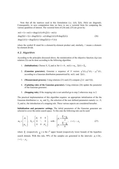
Initialization and parameter settings. The initial parameters of the Gaussian generator are
selected to cover the entire search space. To this end, the following rule can be used:
m
0
qi
+ q
⎡
⎧
μ ⎤ ⎡
i
1 σ 0 0 ⎤
1
i =
⎪
⎪μ
⎢ ⎥ ⎢ ⎥
2
=
⎢
M
⎥
, Σ0
=
⎢
0 O 0
⎥
, with : ⎨ , i = 1,
L,
n
qi
− q
⎢μ
i
n ⎥ ⎢ 0 0 σ ⎪
⎣ q ⎦ ⎣
n ⎥ q ⎦ ⎪
σ i =
⎩ 6
where q i (respectively
q
1
2
(26)
N
(27)
q ) is the i
i
th upper bound (respectively lower bound) of the hyperbox
search domain. With this rule, 99% of the samples are generated in the intervals: μi ± 3σ
i ,
i = 1, L,
n .
q