q - Rosario Toscano - Free

More documents

Recommendations

Info

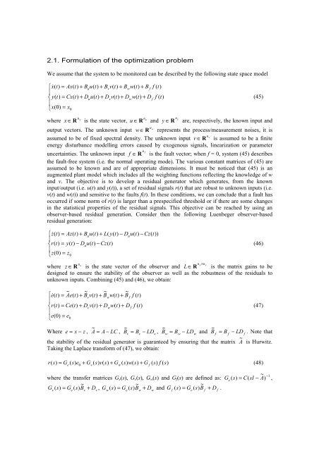
2.1. Formulation of the optimization problem We assume that the system to be monitored can be described by the following state space model ⎧x& ( t) = Ax( t) + Buu( t) + Bvv( t) + Bww( t) + B f f ( t) ⎪ ⎨y( t) = Cx( t) + Duu( t) + Dvv( t) + Dww( t) + D f f ( t) ⎪ ⎩x( 0) = x0 where x n u x ∈ R is the state vector, u ∈ R and n nw n y R (45) y ∈ are, respectively, the known input and output vectors. The unknown input w ∈ R represents the process/measurement noises, it is nv assumed to be of fixed spectral density. The unknown input v ∈ R is assumed to be a finite energy disturbance modelling errors caused by exogenous signals, linearization or parameter n f uncertainties. The unknown input f ∈ R is the fault vector; when f = 0, system (45) describes the fault-free system (i.e. the normal operating mode). The various constant matrices of (45) are assumed to be known and are of appropriate dimensions. It must be noticed that (45) is an augmented plant model which includes all the weighting functions reflecting the knowledge of w and v. The objective is to develop a residual generator which generates, from the known input/output (i.e. u(t) and y(t)), a set of residual signals r(t) that are robust to unknown inputs (i.e. v(t) and w(t)) and sensitive to the faults f(t). In these conditions, we can conclude that a fault has occurred if some norm of r(t) is larger than a prespecified threshold or if there are some changes in the statistical properties of the residual signals. This objective can be reached by using an observer-based residual generation. Consider then the following Luenbeger observer-based residual generation: ⎧z& ( t) = Az( t) + Buu( t) + L( y( t) − Duu( t) − Cz( t)) ⎪ ⎨r( t) = y( t) − Duu( t) − Cz( t) ⎪ ⎩z( 0) = z0 n x y where z ∈ R is the state vector of the observer and L ∈ R is the matrix gains to be designed to ensure the stability of the observer as well as the robustness of the residuals to unknown inputs. Combining (45) and (46), we obtain: ~ ~ ~ ~ ⎧e& ( t) = Ae( t) + Bvv( t) + Bww( t) + B f f ( t) ⎪ ⎨r( t) = Ce( t) + Dvv( t) + Dww( t) + D f f ( t) ⎪ ⎩e( 0) = e0 ~ ~ ~ ~ Where e = x − z , A = A − LC , Bv = Bv − LDv , Bw = Bw − LDw and B f = B f − LD f . Note that the stability of the residual generator is guaranteed by ensuring that the matrix A ~ is Hurwitz. Taking the Laplace transform of (47), we obtain: r e v w f ( s) = G ( s) e0 + G ( s) v( s) + G ( s) w( s) + G ( s) f ( s) (48) nx × n where the transfer matrices Ge(s), Gv(s), Gw(s) and Gf(s) are defined as: ~ ~ ~ G v ( s) = Ge ( s) Bv + Dv , G w( s) = Ge ( s) Bw + Dw and G f ( s) = Ge ( s) B f + D f . G e (46) (47) ~ ( s) = C( sI − A) −1 ,
We want the residual r insensitive to unknown inputs and initial conditions, and sensitive to faults. The stability of the observer will ensure the decay to zero of the effect of nonzero initial conditions e0. Robustness as well as insensitivity to load disturbance can be achieved by satisfying ( s, L) ≤ γ , with γ as small as possible. However, this kind of requirement can G v ∞ also lead to reduction of sensitivity to faults and to an increase of sensitivity to noise. Thus, in addition to ( s, L) ≤ γ , we have to minimize the influence of noise and to maximize the G v ∞ effect of faults. This can be done by solving the following mixed H2/H∞ optimization problem: Minimize Subject to: J mix L = Gw( s, L) ( L) = G ( s, L) g ( L) = G ( s, L) 1 g ( L) = arg max 2 f ⎡ q ⎢ 2 ∞ { Re( λ ( L)), ∀i} q q n [ q ] = ⎢ 21 L 2 y ⎥, q ≤ q ≤ q ij v λi ( L) 11 ⎢ M ⎢ ⎢q ⎣ nx 1 ∞ L M L − γ ≤ 0 i q q 1n y M nxn y ⎤ ⎥ ⎥ ⎥ ⎥⎦ − λ where L = [qij] is the matrix of decision variables, q and q are the bounds of the hyperbox search domain. In the constraint g2(L), the quantity λi(L) denotes the i th pole of the observer. The parameter γ, is used to trade off between detection performance and noise sensitivity. 2.2. Numerical experiments Consider the problem of fault detection in a four-tank process. The state-space process model is given by: ⎡− 0. 0159 ⎢ 0 x& ( t) = ⎢ 0 ⎢ ⎢⎣ 0 ⎡ 0 ⎢ 0 + ⎢ − 0. 0357 ⎢ ⎢⎣ 0 0 − 0. 0111 0 0 0. 0419 0 ⎤ 0 ⎥ ⎥v( t), 0 ⎥ − 0. 0313⎥⎦ 0 − 0. 0419 0 ⎡0. 5 y( t) = ⎢ ⎣ 0 0 0. 5 min i, j 0 0 ≤ 0 0 ⎤ ⎡0. 0833 0. 0333 ⎥ ⎢ 0 ⎥x( t) + ⎢ 0 0 ⎥ ⎢ − 0. 0333⎥⎦ ⎢⎣ 0. 0312 0⎤ x( t) + w( t) 0⎥ ⎦ 0 ⎤ 0. 0718⎥ ⎥( u( t) + f ( t)) 0. 0479 ⎥ 0 ⎥⎦ where the state vector x = [x1 x2 x3 x4] T represents the level of water in the tanks, the control input u = [u1 u2] T is the voltage applied to the pumps, f = [f1 f2] T is the fault vector associated to the pumps, v = [v1 v2] T is the disturbance vector and w = [w1 w2] T is the measurement noise vector. The objective is to detect the actuator fault f in the presence of a disturbance v and the measurement noise w. To evaluate the performance of the residual generator, a fault f1 and a disturbance v1 are applied (see Figure 12). (50) (49)
Page 1 and 2: Stochastic Stochastic Methods Metho
Page 3 and 4: The problem is then how to tune the
Page 5 and 6: where k T > 0 is a normalizing cons
Page 7 and 8: Number of repetitions of the Metrop
Page 9 and 10: where q1 and q2 are coded with 12 b
Page 11 and 12: i i i i Inversely, the decoding of
Page 13 and 14: Each individual of the population o
Page 15 and 16: 3. Particle Swarm Optimization (PSO
Page 17 and 18: The inertia weight. The inertia coe
Page 19 and 20: 3.3. Advantages and disadvantages o
Page 21 and 22: Our ignorance about the optimum can
Page 23 and 24: Note that all the matrices used in
Page 25 and 26: 5.1. Comparison of HKA with SA, GA
Page 27 and 28: 5.2. Comparison of HKA with other m
Page 29 and 30: and: c ( q) = 1 0. 10471, 7 G = 1.
Page 31 and 32: and K(s) is, for instance, the tran
Page 33 and 34: where [ ] T q = q1 q2 q3 q is the v
Page 35: where q is the decision vector whic
Page 39 and 40: For comparison, Figure 14 shows the
Page 41 and 42: Constrained test problem (F8) (3 va
Page 43 and 44: Coello, C.A.C. (2002). Theoretical
Page 45: Siarry, P., Berthiau, G., Durbin, F

q - Rosario Toscano - Free

You also want an ePaper? Increase the reach of your titles

Delete template?

Save as template?