q - Rosario Toscano - Free

More documents

Recommendations

Info

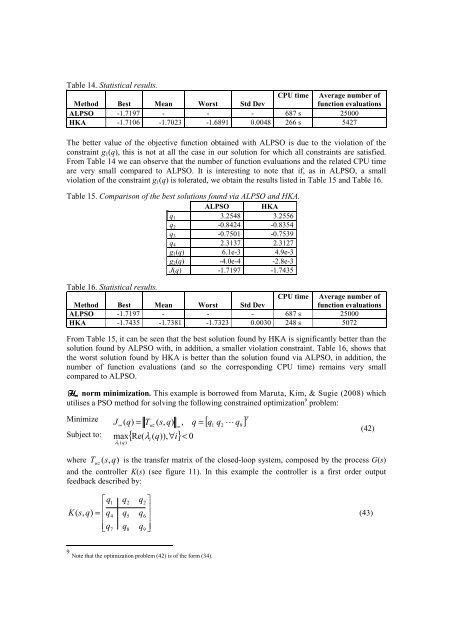
Table 14. Statistical results. CPU time Average number of Method Best Mean Worst Std Dev function evaluations ALPSO -1.7197 - - - 687 s 25000 HKA -1.7106 -1.7023 -1.6891 0.0048 266 s 5427 The better value of the objective function obtained with ALPSO is due to the violation of the constraint g1(q), this is not at all the case in our solution for which all constraints are satisfied. From Table 14 we can observe that the number of function evaluations and the related CPU time are very small compared to ALPSO. It is interesting to note that if, as in ALPSO, a small violation of the constraint g1(q) is tolerated, we obtain the results listed in Table 15 and Table 16. Table 15. Comparison of the best solutions found via ALPSO and HKA. ALPSO HKA q1 3.2548 3.2556 q2 -0.8424 -0.8354 q3 -0.7501 -0.7539 q4 2.3137 2.3127 g1(q) 6.1e-3 4.9e-3 g2(q) -4.0e-4 -2.8e-3 J(q) -1.7197 -1.7435 Table 16. Statistical results. CPU time Average number of Method Best Mean Worst Std Dev function evaluations ALPSO -1.7197 - - - 687 s 25000 HKA -1.7435 -1.7381 -1.7323 0.0030 248 s 5072 From Table 15, it can be seen that the best solution found by HKA is significantly better than the solution found by ALPSO with, in addition, a smaller violation constraint. Table 16, shows that the worst solution found by HKA is better than the solution found via ALPSO, in addition, the number of function evaluations (and so the corresponding CPU time) remains very small compared to ALPSO. HHHH∞ norm minimization. 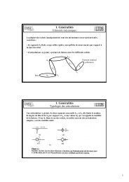This example is borrowed from Maruta, Kim, & Sugie (2008) which utilises a PSO method for solving the following constrained optimization 9 problem: Minimize [ ] T J ∞ ( q) = Twz ( s, q) , ∞ q = q1 q2 L q9 max Re( λi ( q)), ∀i λi ( q) < Subject to: { } 0 where Twz ( s, q) is the transfer matrix of the closed-loop system, composed by the process G(s) and the controller K(s) (see figure 11). In this example the controller is a first order output feedback described by: ⎡q1 q2 q2 ⎤ K ( s, q) = ⎢ ⎥ ⎢ q4 q5 q6 (43) ⎥ ⎢⎣ q ⎥ 7 q8 q9 ⎦ 9 Note that the optimization problem (42) is of the form (34). (42)
where q is the decision vector which have to be set in order to satisfy (42). The transfer matrix G(s) of the process to be controlled is given by: ⎡ 0 ⎢ ⎢ 1. 5 ⎢ −12. 0 ⎢ ⎢− 0. 852 ⎢ 0 ⎢ ⎢ 0 ⎢ 0 G(s) = ⎢ ⎢ 0 ⎢ 1 ⎢ ⎢ 0 ⎢ ⎢ 0 ⎢ 0 ⎢ ⎢ 1 ⎢ ⎣ 0 0 −1. 5 12. 0 0. 29 0 0 0 0 0 1 0 0 0 1 1. 0 0 − 0. 6 0 0 0 0 0 0 0 0 0 0 0 0 0. 0057 − 0. 0344 − 0. 014 0 0 0 0 0 0 0 0 0 0 0 1. 5 −12. 0 − 0. 29 − 0. 73 0 0 0 0 0 0 0 0 0 0 0 0 0 2. 8289 −1. 25 0 0 0 0 0 0 0 0 0 0 0 0 0 0 −1000 0 0 0 0 0 −139. 0206 0 0 0 0 0 0 0 0 −1000 0 0 0 0 0 −139. 0206 0 0 0 0 0. 1146 4. 0 0 0 0 0 0 0 0 0 0 0 0 0 0 0 1024 0 0 0 0 0 142. 8571 0 0 0 0 0 0 0 0 1024 0 0 0 0 0 142. 8571 0 0. 16 −19. 0 − 0. 0115 0 0 0 0 0 0 0. 01 0 0 0 0 0. 8 − 3. 0 ⎤ ⎥ ⎥ ⎥ ⎥ ⎥ ⎥ ⎥ ⎥ ⎥ ⎥ ⎥ ⎥ ⎥ ⎥ ⎥ ⎥ ⎥ ⎥ ⎥ ⎥ ⎦ − 0. 0087 The objective is to find a stabilizing q which minimizes the H∞ norm of the closed-loop transfer matrix. The search space is: −15 ≤ xi ≤15, i = 1, K9 . We performed the minimization 35 times (N = 50, Nξ = 2, α = 0.5) and we compared our results with those obtained in Maruta, Kim, & Sugie (2008) . Tables 17 and 18 summarize de results of this experiment. Table 17. Comparison of the best solutions found via PSO and HKA. q1 q2 q3 q4 q5 q6 q7 q8 q9 PSO -21.1183 -1.5886 11.0822 -2.9907 0.4011 -0.5268 -20.0049 0.4298 -0.9064 HKA -33.1421 -2.2374 14.8739 -3.2335 0.4748 -0.6776 -25.5573 0.5167 -0.0761 Table 18. Statistical results (comparison between PSO and HKA). Method Best Mean Worst Std Dev CPU-time Nb iter PSO 1.7092 1.7775 2.3732 0.0996 650 seconds - HKA 1.6634 1.7326 2.2377 0.0964 45 seconds 126 From Table 18, we can see that the best solution found by HKA is significantly better than the solution found in Maruta, Kim, & Sugie (2008). The same is true for the mean, worst and standard deviation. In addition, the computation time is very very small compared to PSO. 2. Robust residual generator In this section, we introduce a simple but effective synthesis strategy for observers based faults detection in linear time-invariant (LTI) systems which are simultaneously affected by two classes of unknown inputs: Noises having fixed spectral densities and unknown finite energy disturbances Khosrowjerdi, Nikoukhah & Safari-Shad, (2005). The problem of designing such an observer, also called a residual generator, will be formulated as a mixed H2/H∞ optimization problem. This is done to obtain an optimal residual generator, i.e. with minimal sensitivity to unknown inputs. Unfortunately, there is no known solution to this difficult optimization problem. Finding such a residual generator is known to be computationally intractable via the conventional techniques (<strong>Toscano</strong> & Lyonnet, 2009). This is mainly due to the non-convexity of the resulting optimization problem. To solve this kind of problem easily and directly, without using any complicated mathematical manipulations, we utilize stochastic methods for the resolution of the underlying constrained non-convex optimization problem. A numerical example is given to illustrate the advantage of the mixed H2/H∞ optimization approach against existing techniques which are based on optimization of H2 or H∞ criteria. 0 0 0 0 0 0 0 0. 01 0 0 (44)
Page 1 and 2: Stochastic Stochastic Methods Metho
Page 3 and 4: The problem is then how to tune the
Page 5 and 6: where k T > 0 is a normalizing cons
Page 7 and 8: Number of repetitions of the Metrop
Page 9 and 10: where q1 and q2 are coded with 12 b
Page 11 and 12: i i i i Inversely, the decoding of
Page 13 and 14: Each individual of the population o
Page 15 and 16: 3. Particle Swarm Optimization (PSO
Page 17 and 18: The inertia weight. The inertia coe
Page 19 and 20: 3.3. Advantages and disadvantages o
Page 21 and 22: Our ignorance about the optimum can
Page 23 and 24: Note that all the matrices used in
Page 25 and 26: 5.1. Comparison of HKA with SA, GA
Page 27 and 28: 5.2. Comparison of HKA with other m
Page 29 and 30: and: c ( q) = 1 0. 10471, 7 G = 1.
Page 31 and 32: and K(s) is, for instance, the tran
Page 33: where [ ] T q = q1 q2 q3 q is the v
Page 37 and 38: We want the residual r insensitive
Page 39 and 40: For comparison, Figure 14 shows the
Page 41 and 42: Constrained test problem (F8) (3 va
Page 43 and 44: Coello, C.A.C. (2002). Theoretical
Page 45: Siarry, P., Berthiau, G., Durbin, F

q - Rosario Toscano - Free

Create successful ePaper yourself

Delete template?

Save as template?