II - FEFlow

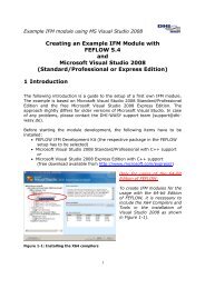
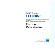
DHI-WASY Software 

FEFLOW ® 

6 

Finite Element Subsurface Flow 

& Transport Simulation System 

Installation Guide & Demonstration Exercise

Copyright notice: 

No part of this manual may be photocopied, reproduced, or translated without written permission of 

the developer and distributor DHI-WASY GmbH. 

Copyright © 2010 DHI-WASY GmbH Berlin – all rights reserved. 

DHI-WASY, FEFLOW and WGEO are registered trademarks of DHI-WASY GmbH. 

DHI-WASY GmbH 

Waltersdorfer Straße 105, 12526 Berlin, Germany 

Phone: +49-(0)30-67 99 98-0, 

Fax: +49-(0)30-67 99 98-99 

E-Mail: mail@dhi-wasy.de 

Internet: www.feflow.info 

www.dhigroup.com 

2

Contents 

I Installation Guide 4 

I.1 Introduction 4 

I.2 Installing FEFLOW (Windows) 5 

l.2.1 Introduction 5 

I.2.2 System recommendations 6 

I.2.3 FEFLOW Installation 6 

I.2.4 Demo Data Installation 7 

l.2.5 Installation of the X server 

Exceed 2006 7 

l.2.6 Installation of the Network License 

Manager NetLM 8 

I.2.7 License installation 8 

I.3 Installing FEFLOW (Linux) 9 

I.4 Installation Packages 10 

II Demonstration Exercise 11 

II.1 Introduction 11 

II.1.1 About FEFLOW 11 

II.1.2 Scope and Structure 11 

II.1.3 Terms and Notations 12 

II.1.4 Requirements 12 

II.1.5 Model Scenario 13 

II.2 Getting Started 14 

II.2.1 Starting FEFLOW 14 

II.2.2 The FEFLOW 6 User Interface 14 

II.3 Geometry 15 

II.3.1 Maps and Model Bounds 15 

II.3.2 Supermesh 16 

II.3.3 Finite element-mesh 19 

II.3.4 Expansion to 3D 21 

II.4 Problem settings 28 

II.5 Model Parameters 30 

II.5.1 Initial conditions 30 

II.5.2 Boundary conditions 32 

II.5.3 Material properties 37 

II.6 Simulation 39 

II.7 Flow Transport Model 42 

II.7.1 Problem settings 42 

II.7.2 Initial Conditions 44 

II.7.3 Boundary conditions 45 

II.7.4 Material properties 46 

II.7.5 Vertical resolution 46 

II.7.6 Reference data 48 

II.7.7 Simulation Run 49 

II.7.8 Postprocessing 50 

FEFLOW 6 

3

I Installation Guide 

I.1 Introduction 

The FEFLOW simulation package contains the following 

main programs along with additional software 

tools: 

FEFLOW ® 6.0 

Interactive finite-element simulation system for 

modeling 3D and 2D flow, mass and heat transport 

processes in ground water and the vadose 

zone. 

FEFLOW is provided on DVD for the following 

platforms: 

32-bit operating systems 

• Windows XP, Vista, 7, Server 2003, Server 2008 

• Linux: CentOS 4.6 (RedHat family), OpenSUSE 

11.0 (SUSE family), Ubuntu 8.04 (Debian family) 

64-bit operating systems 

• Windows XP x64 Edition, Vista x64 Edition, 

7 x64 Edition, Server 2003 x64 Edition, 

Server 2008 x64 Edition 

• Linux: CentOS 4.4 (RedHat family), OpenSUSE 

11.0 (SUSE family), Ubuntu 8.04 (Debian family) 

Installation Guide & Demonstration Exercise 

FEFLOW for other Linux distributions may be available 

for download from the FEFLOW website 

www.feflow.info. If you need FEFLOW for another 

Linux distribution, please do not hesitate to contact 

us at support@dhi-wasy.de! 

For evaluation purposes, it is possible to obtain a 

fully functional but time-limited license from DHI- 

WASY, one of the DHI offices, or from your local 

FEFLOW distributor. 

FEFLOW ® Viewer 

FEFLOW Viewer is free software for visualizing 

FEFLOW models and results and for postprocessing 

purposes. FEFLOW Viewer is installed with 

FEFLOW. 

WGEO ® 6.0 

WGEO® is a sophisticated georeferencing, 

geoimaging and coordinate transformation software 

developed by DHI-WASY GmbH. A license 

for WGEO® Basis and the flexible 7-parameter 

transformation comes with each FEFLOW license 

and is installed automatically. 

WGEO® is provided for the Windows platform. 

4

I.2 Installing FEFLOW 

(Windows) 

I.2.1 Introduction 

FEFLOW 6 Standard provides powerful state-ofthe-art 

editing and visualization tools for most 

kinds of applications. As some of the lesser used 

functionality for data input is not yet implemented 

in FEFLOW 6 Standard, FEFLOW 6 Classic is provided 

as a fallback. Convenient tools make it easy 

to switch between the two types of user interface. 

The FEFLOW 6 Classic requires an X server running 

on display number 10 for proper operation. DHI- 

WASY recommends to use Hummingbird Exceed 

2006 for this purpose, a customized version of 

which is available on the FEFLOW DVD. It may only 

be used in conjunction with FEFLOW. 

To run FEFLOW in single-seat mode, the DHI-WASY 

License Manager NetLM has to be installed locally. 

Only NetLM has to be installed on network license 

servers, distributing FEFLOW licenses to clients in 

the network. 

So a typical FEFLOW installation on a Windows 

operating system consists of four steps: 

• Installation of FEFLOW and additional programs 

• Installation of the demo data package 

• Installation of the X server Exceed 2006 (only 

needed for running FEFLOW 6 Classic) 

• Installation of the DHI-WASY license manager 

NetLM 

After inserting the DVD into the DVD drive, an 

overview of the DVD contents is shown automatically. 

If autostart is disabled, run Starter.exe from 

the windows directory on the DVD. 

The hyperlinks in the overview can be used to start 

the different parts of the FEFLOW installation, to 

view the documentation and example movies, and 

to install third-party software. 

FEFLOW is automatically installed as a 32 bit version 

on 32 bit systems, and as 32 and 64 bit versions 

on 64 bit operating systems. 

FEFLOW 6 

5 

I

Installation Guide 

I.2.2 System recommendations 

The following system specifications are recommended 

as a minimum configuration. The 

memory requirements depend on the size and 

complexity of the actual model to be simulated. 

• 512 MB RAM 

• 450 MB of disk space 

• Screen resolution of 1280 x 1024 or higher for 

FEFLOW 6 Classic 

• Separate graphics card with up-to-date graphics 

driver 

I.2.3 FEFLOW Installation 

Start the Windows Installer by clicking on the 

hyperlink FEFLOW Program Files. Click Next after 

each step to proceed to the next step. 

1. A Welcome screen appears first. 


2. In the next step, the License Agreement has to 

be accepted. Please read it carefully before proceeding 

with the installation. 

3. In the License window, choose Demo for testing 

FEFLOW without a license. Select Client if the 

license to be used is installed on a remote 

license server (Network License) and type in the 

name or IP number of the license server. Choose 

Server if a Single Seat License is to be used or if 

the machine is intended to act as a license server 

for a Network License. 

I 

6

4. Select the packages to install. Details about the 

packages can be found on the right of the window 

and on page 10 of this booklet. The 

default installation location is C:\Program 

Files\WASY\FEFLOW 6.0. For specifying a different 

destination directory, click Browse. 

5. Start the installation or go back to change the 

settings. 

6. FEFLOW is installed. This may take several minutes. 

7. Finish the installation by clicking Finish. 

I.2.4 Demo Data Installation 

The demo data installation is started by clicking on 

the hyperlink FEFLOW Demo Data. 

I.2.5 Installation of the X server 

Exceed 2006 

Before installing Hummingbird Exceed for 

FEFLOW, we recommend to manually deinstall all 

previous versions of Exceed. 

FEFLOW 6 

7 

I

There is only one 

dongle for each 

copy of FEFLOW. 

If the dongle is lost, it can 

only be replaced by purchasing 

a new license of 

FEFLOW! 


Start the installation by clicking on the corresponding 

hyperlink. The setup installs all parts of 

Exceed 2006 (version 11) required for running 

FEFLOW. The basic X server settings are customized 

for running FEFLOW. 

Terminal Server installation 

On Terminal Server, the installation of Exceed 

2006 has to be performed in a different way: 

Follow the procedure described in 

ConnectivityInstallation.pdf (Chapter 3, Installation 

on a Terminal Server), located in the windows\exceed 

directory of the FEFLOW DVD. 

I.2.6 Installation of the Network 

License Manager NetLM 

Before installing the Network License Manager 

NetLM we recommend to deinstall all previous 

versions of NetLM. 

The installation is started by clicking on the hyperlink 

License Manager NetLM. Follow the instructions 

in the installation dialog. 


I.2.7 License installation 

This step can be skipped for working in Demo 

mode only. All license installations have to be done 

with administrator privileges. 

Make sure that the firewall allows (local) TCP/IP 

connections on port 1800. 

• Install the dongle (hardware lock) on the USB 

port or parallel port resp. Start the DHI-WASY 

License Administration tool by clicking on the 

WASY License Administration entry in the All 

Programs\WASY group of the Windows start 

menu. 

I 

8

For the 64 bit version 

of FEFLOW, a 

HASP HL USB 

dongle is required. If you do 

not already have such a 

dongle, please contact your 

FEFLOW distributor or DHI- 

WASY for a dongle 

exchange! 

For the version, 

please note that 

you have to use 

“6.0x” because your license 

is valid for all sub-versions 

of FEFLOW 6.0. 

• In the tree view on the left side, select Dongle 

license in the FEFLOW 6.0 branch. In the 

Hostname or IP address field, insert localhost if 

the dongle is installed locally, or insert the name 

or the IP number of the remote license manager. 

• Click Connect. Check whether the number 

returned in the field HOSTID is identical to the 

number on the FEFLOW license sheet. In case 

that multiple dongles of the same brand are 

connected, a HOSTID mismatch may occur. In 

this case remove all dongles except the DHI- 

WASY dongle. 

• Switch to the Licenses tab and enter the license 

information from the FEFLOW license sheet. The 

license information can be pasted from the clipboard 

if the license has been received digitally. 

Copy the selected section in the license document 

to the clipboard and use on the Paste 

license from clipboard button to insert all the 

license information at once. Please also make 

sure that the same license type as on the license 

sheet is selected: 

• Single seat license – FEFLOW can be run only 

on the computer the dongle is attached to. 

• Network license – FEFLOW can be used on any 

computer connected to the license server via 

TCP/IP network (LAN or WAN/internet). 

• Click Install. A message box indicates that the 

license has been successfully installed. If the 

installation was not successful, check all the 

license information in comparison to the information 

provided on the license sheet. The information 

has to be identical in all details. 

• Click OK to close the License Administration dialog. 

• Choose FEFLOW 6.0 from the WASY program 

group or double click on the desktop icon to 

start FEFLOW. 

Using a Network License for FEFLOW, the WASY 

License Manager can be installed on any computer 

within the network (LAN or WAN) without the 

complete FEFLOW installation. Clients need TCP/IP 

connection on port 1800 to have access to the 

license server. 

I.3 Installing FEFLOW 

(Linux) 

• Browse to the linux directory on the DVD. 

• Browse to the sub directory corresponding to 

your Linux distribution. 

• For a full installation, use the following command: 

rpm -i *.rpm 

• For deinstalling all WASY packages, use rpm - 

e ‘rpm -qa | grep ’^wasy-’‘ 

• Note that you may need root privileges to perform 

these commands. 

FEFLOW 6 

9 

I

WGEO Basis is 

licensed automatically 

with 

FEFLOW. If a license dialog 

show up, just click on 

Cancel. 


I.4 Installation Packages 

• Packages for installation can be selected during 

the first installation or by re-running the installation 

in Modify mode. 

• A description for each package is shown in the 

right part of the Select feature dialog of the 

installation by selecting one of the packages. 

• The following packages are available: 

FEFLOW 

FEFLOW program files - required for running 

FEFLOW 

• Help - FEFLOW help system 

• Interface Manager SDK - development kit for 

the open programming interface IFM (required 

for plug-in development) 

• Desktop shortcut icon - WGEO icon on the 

Windows desktop 


WGEO 

Georeferencing, geoimaging and transformation 

software - a WGEO license is installed automatically. 

• WGEO help - online help system 

• German Transformations - coordinate transformation 

routines for Germany (may require separate 

licensing) 

• Desktop shortcut icon - WGEO icon on the 

Windows desktop 

Plot Assistant 

GIS-like software for producing plots with FEFLOW 

data. 

Data Tools 

Scripts for data checking and format conversion. 

In the demo data installation there are the following 

packages: 

• Examples - example models 

• Exercise - data for the demonstration exercise 

• Tutorial - data for the tutorials (User Manual) 

• Benchmarks - benchmark models 

I 

10

II Demonstration Exercise 

II.1 Introduction 

II.1.1 About FEFLOW 

FEFLOW (Finite Element subsurface FLOW and 

transport system) is an interactive groundwater 

modeling system for 

• three-dimensional and two-dimensional 

• areal and cross-sectional (horizontal, vertical or 

axisymmetric) 

• fluid density-coupled, also thermohaline, or 

uncoupled 

• variably saturated 

• transient or steady state 

• flow, mass and heat transport 

• reactive multi-species transport 

in subsurface water resources with or without one 

or multiple free surfaces. 

FEFLOW can be efficiently used to describe the 

spatial and temporal distribution and reactions of 

groundwater contaminants, to model geothermal 

processes, to estimate the duration and travel 

times of chemical species in aquifers, to plan and 

design remediation strategies and interception 

techniques, and to assist in designing alternatives 

and effective monitoring schemes. 

Sophisticated interfaces to GIS and CAD data as well 

as simple text formats are provided. 

The option to use and develop user-specific plugins 

via the programming interface (Interface 

Manager IFM) allows the addition of external code 

or even external programs to FEFLOW. 

FEFLOW is available for WINDOWS systems as well 

as for different Linux distributions. 

Since its first appearance in 1979 FEFLOW has 

been continuously extended and improved. It is 

consistently maintained and further developed by 

a team of experts at DHI-WASY. FEFLOW is used 

worldwide as a high-end groundwater modeling 

tool at universities, research institutes, government 

agencies and engineering companies. 

For additional information about FEFLOW please 

do not hesitate to contact your local DHI office, 

one of the FEFLOW distributors, DHI-WASY, or 

have a look at the FEFLOW web site 

http://www.feflow.info. 

II.1.2 Scope and Structure 

This exercise provides a step-by-step description 

of the setup, simulation, and post processing of a 

three-dimensional flow and transport model based 

on (simplyfied) real-world data, showing the 

philosopy and handling of the FEFLOW user interface. 

FEFLOW 6 

11

You can skip any 

of the steps in this 

exercise by loading 

already prepared files at 

certain stages. These files 

are not necessarily ready to 

run in the simulator. 

For following the 

exercise, the demo 

data files for 

FEFLOW have to be installed. 

The demo data installation 

package is available 

on the FEFLOW DVD as 

well as on the FEFLOW web 

site for download. 

Demonstration Exercise 

The demonstration exercise is not intended as an 

introduction to groundwater modeling itself. 

Therefore, some background knowledge of 

groundwater modeling is required, or common 

literature should be consulted in parallel. 

The exercise covers the following work steps: 

• Import of background maps 

• Definition of the basic model geometry 

• Generation of a 2D finite-element mesh 

• Expansion of the mesh to 3D 

• Setup of a steady-state flow and transient transport 

model, including initial conditions, boundary 

conditions and material properties 

• Import of GIS data and regionalization 

• Simulation run 

• Results visualization and post processing 

II.1.3 Terms and Notations 

In addition to the verbal description of the required 

screen actions this exercise makes use of some 

icons. They are intended to assist in relating the 

written description to the graphical information 

provided by FEFLOW. The icons refer to the kind 

of setting to be done: 

main menu 

context menu 


toolbar 

panel 

button 

input box for text or numbers 

switch toggle 

radio button 

checkbox 

All file names are printed in bold red, map names 

are printed in red, numbers to be input in bold 

green. Keyboard keys are referenced in 

style. All required files are available in the FEFLOW 

demo data. The symbol indicates an intermediary 

stage where either a prepared file can be 

loaded to resume this exercise or - if working with 

a license - the model can be saved. Thus the exercise 

does not have to be done in one step even in 

demo mode. 

II.1.4 Requirements 

If not already done, please install the FEFLOW software 

including the demo data package. A license is 

not necessary to run this tutorial (FEFLOW can be run 

in demo mode). 

The latest version of FEFLOW can be downloaded 

from the website www.feflow.info. In case of any 

problems or additional questions please do not hesitate 

to contact the FEFLOW technical support 

(support@dhi-wasy.de ). 

II 

12

II.1.5 Model Scenario 

A fictitious contaminant has been detected near 

the small town of Friedrichshagen, in the southeast 

of Berlin, Germany. An increasing concentration 

of nitrate can be observed in two water supply 

wells. There are two potential sources of the contamination: 

The first are abandoned sewage fields 

close to a waste-water treatment plant located in 

an industrial area northeast of town. The other 

possible source is an abandoned waste-disposal 

site further east. 

A three-dimensional groundwater flow and contaminant 

transport model is set up to evaluate the 

overall threat to groundwater quality, and to quantify 

the potential pollution. First, the model domain 

needs to be defined. The town is surrounded by 

many natural flow boundaries, such as rivers and 

lakes. There are two small rivers that run northsouth 

on either side of Friedrichshagen that can 

act as the eastern and western boundaries. The 

lake Müggelsee can limit the model domain to the 

south. The northern boundary is chosen along an 

east-west hydraulic contour line of groundwater 

level north of the two potential sources of the contamination. 

The geology of the study area is comprised of 

Quaternary sediments. The hydrogeologic system 

contains two main aquifers separated by an 

aquitard. The top hydrostratigraphic unit is considered 

to be a sandy unconfined aquifer up to 7 

meters thick. The second aquifer located below 

the clayey aquitard has an average thickness of 

approximately 30 meters. 

The northern part of the model area is primarily 

used for agriculture, whereas the southern portion 

is dominated by forest. In both parts, significant 

urbanized areas exist. 

FEFLOW 6 

13 

II


II.2 Getting Started 

II.2.1 Starting FEFLOW 

On Windows Systems 

• Start FEFLOW 6.0 via the corresponding desktop 

icon or the startup menu entry. 

On Linux Systems 

• Type feflow60q in a console window and press 

. 

If no FEFLOW license is available, FEFLOW asks 

whether to start in demo mode. The demo mode 

does not allow loading and saving of files with 

more than 500 nodes, and it does not allow to 

execute the simulation run. Specially prepared 

demo files coming with FEFLOW are an exception. 

Such files are provided for this example so that the 

model setup can be interrupted and picked up 

again, and the simulation runs can be performed. 

II.2.2 FEFLOW 6 User Interface 

The user interface components are organized in a 

main menu, toolbars, panels, view windows, and 

dialogs. 

While the main menu is always visible, the other 

parts of the interface can be customized, adding 

or hiding particular toolbars and panels by using 


the menu command View > Panels 

and View > Toolbars, respectively. Please keep 

in mind that not all panels and toolbars are displayed 

by default. Thus this exersice may require 

to access a function in a toolbar or panel that is 

not visible at that moment. The toolbar or panel 

has to be added then. 

View windows display a certain type of view on 

the model and its properties. There are four different 

types of view windows: Supermesh view, FE- 

Slice view, 3D view and Cross-Section view. Different 

kinds of tools are linked to the different view types. 

View windows can be closed via the corresponding 

button in the view frame. New view windows 

can be opened by selecting Window > New 

and choosing the respective view window type. 

The last type of user interface component relevant 

for the exercise are diagrams. Looking very similar 

to panels, they contain plots of time curves. 

Missing diagram windows can be added to the 

user interface by opening View > Diagram from 


14

the menu and choosing the required diagram 

from the list. 

Last, but not least it might be worth to mention 

that all steps done in FEFLOW can be undone and 

redone via the corresponding toolbar buttons. 

There is no limit on the number of undo steps. 

II.3 Geometry 

II.3.1 Maps and Model Bounds 

When FEFLOW starts, by default a new document 

is opened. A new document can also be 

created using the menu command File > 

New or the New button in the Standard 

toolbar. 

The first step of model setup is the definition of 

the Initial Domain Bounds. This can be done manually, 

or by loading georeferenced maps. 

All necessary files for this exercise are provided with 

the FEFLOW Demo Data package and are located 

in the project folder demo/exercise/standard. The 

map files are found in the subdirectory 

import+export. 

Click on Load map(s). Load all the following 

maps at once (by holding on the keyboard) 

to ensure that FEFLOW uses the bounding box of 

all the maps to define the initial domain bounds. 

The particular map files that are needed now are: 

• topography_rectified.tif (a georeferenced raster 

image of the model area for better orientation) 

• model_area.shp (a polygon that denotes the 

outer model boundary) 

• sewage_fields.dxf (the footprint of the sewage 

fields as a polygon) 

• waste_disposal.shp (the outline of the waste 

disposal site) 

• demo_wells.shp (the positions of the wells) 

Some of these maps will also be used for model 

parameterization later on. 

After import, the maps are listed in the Maps 

panel, sorted by their file type (see figure). A double 

click on the Geo-TIFF topography_rectified adds the 

georeferenced topographic map to the active 

Supermesh view window. 

FEFLOW 6 

15 

II


Except for the map sewage-fields, all other maps are 

ESRI shape files. These vector files occupy their own 

branch in the tree, each with a default map layer. 

Double-click on all the Default layer entries to add 

the visualization layers of the shape files to the 

Supermesh view. 

Now have a closer look at a second panel, the 

View Components panel. This panel lists the components 

that are currently plotted in the active view 

window. 

When having double-clicked on the maps in the 

Maps panel, the maps have been added to the 

tree in the View Components panel. 


The drawing order of maps can be modified by 

dragging them with the mouse to another position 

in the tree (this might become necessary as 

the model area polygon may overlay the polygons 

of the mass sources). The topmost map is drawn 

on top. 

To switch a map on and off, the checkbox in front 

of the map name can be checked/unchecked. 

Checking/unchecking the checkbox of an entire 

branch all the maps in this branch become visible/invisible 

at the same time. 

The topographic map has mainly been loaded for 

providing a regional context. For more clarity, it 

can be switched off before starting with the following 

operations. Make sure that the other maps 

are visible. 

II.3.2 Supermesh 

In the simplest case, the supermesh contains a definition 

of the outer model boundary. In addition, 

geometrical features such as the position of pumping 

wells, the limits of areas with different properties 

or the courses of rivers can be included to 

be considered for the generation of the finite-element 

mesh. Additionally, the polygons, lines and 

points specified in the supermesh can be used later 

on to assign boundary conditions or material properties. 


16

As mentioned above, a supermesh may contain 

three types of features: 

• polygons 

• lines 

• points 

At least one polygon has to be created to define 

the model area boundaries. 

The editing tools are found in the Mesh Editor 

toolbar: 

Outer boundary 

This polygon can be directly loaded from the map 

model_area. In the Maps panel, open the context 

menu of this map (with a right-click on the 

map name) and choose Convert to > 

Supermesh Polygons. 

A first supermesh polygon is automatically generated, 

using the information in the map. Thus a 

valid supermesh exists that would allow the generation 

of a finite-element mesh. However, two 

more features are to be included in the supermesh 

for this example: the well locations and the areas 

of contamination sources. 

Well locations 

The positions of the wells can be imported directly 

from a map as well. Open the context menu of 

the map demo_wells and choose Convert to > 

Supermesh Points. 

The points immediately appear as red dots in the 

Supermesh view. 

FEFLOW 6 

17 

II


exercise_fri1.smh 

Contamination sources 

The estimated source areas of the contaminations 

are to be represented in the supermesh by polygons. 

To avoid overlapping of polygons (which is 

not allowed at any editing stage), the initial polygon 

covering the entire model area is partitioned 

manually. 

Click on Split Polygons. This tool allows to split 

an existing polygon along a polyline to be drawn. 

Here, it is used to separate the two areas of contamination 

sources from the existing polygon. 


Start with the eastern source of contamination (the 

former waste-disposal site). 

The splitting has to start and end at an already 

existing polygon border (but not necessarily at 

already existing polygon nodes). As the contamination 

sources are located completely inside the 

model area, two cuts are necessary when carving 

the new polygon from the existing one. 

By selecting the map waste_disposal from the dropdown 

list in the Mesh Editor toolbar and activating 

Snap to points, a snapping mode is 

employed for the geometrical information in the 

corresponding background map. The mouse cursor 

snaps to the exact position of the polygon map 

nodes when clicking close to them. This allows for 

accurate digitizing. 


18

Zooming functions 

can be used 

at any time. Press 

and hold the right mouse 

button, move the mouse 

up/down). Pan by pressing 

and holding the mouse 

wheel and moving the 

mouse to any direction. 

Also the mouse wheel may 

be used for zooming. 

The first cut starts on an 

arbitrary point on the 

model boundary, then 

going half-way around the 

contamination source and 

returning to the model 

boundary on the other side 

(see figure, red arrows). The 

second cut completes the 

polygon by cutting along 

the missing part of the border of the outline of the 

waste disposal (see figure, green arrows). 

For the next step, select the map sewage_fields for 

snapping in the dropdown list in the 

Mesh Editor toolbar. 

In the same way as before the polygon for the 

sewage fields, the western source of contamination, 

is created. Use the Split Polygons tool to 

create polygon borders along its outline. 

An example supermesh setup for both the disposal 

site and the sewage fields is shown in the following 

figure. 

Corrections 

Accidently created polygons, lines, or points can 

be selected by using the Select tool. They can 

be deleted hitting on the keyboard. 

Misplaced nodes in polygons or lines can be 

removed during digitizing by going back to the 

last correct node of the feature and clicking on it. 

The position of a point can be corrected after a 

polygon or line has been finished by using the 

Move node tool to shift its position (the snapping 

mode can be used here as well). 


II.3.3 Finite element-mesh 

Once the outer boundary and other geometrical 

constraints have been defined in the supermesh, 

the finite-element mesh can be generated. 

All necessary tools can be found in the 

Mesh Generator toolbar. 

First, one of the mesh generation algorithms provided 

by FEFLOW is chosen from the drop-down 

list in the Mesh Generator toolbar. 

For this example, choose Gridbuilder. Click 

Generate Mesh to start mesh generation. 

FEFLOW 6 

19 

II

Besides refinement 

along polygon 

borders, 

FEFLOW also provides the 

means to edit the desired 

relative mesh density on a 

polygon-by-polygon basis. 


A new FE-Slice view is automatically opened, 

depicting the resulting finite-element mesh. 

For our purpose, especially for the simulation of 

contaminant transport, this initially generated 

mesh does not seem to be appropriate. A finer spatial 

resolution is required. 

Activate the Supermesh view again so that the 

Mesh Generator and Supermesh toolbar 

become visible again. 

In the Mesh Generator toolbar, enter 6000 

as the Total Number and hit Generate Mesh 

again. The finite-element mesh in the FE-Slice view 

is updated, showing a much finer discretization 

now. 

Local refinement 

First, special attention should be paid to the areas 

of the contamination sources. At their borders, the 

occurrence of high concentration gradients is likely, 

possibly requiring an even finer spatial resolution 

to avoid oscillations in the solution. Consequently, 

the mesh needs local refinement along the polygon 

outlines. 

Second, at the pumping wells steep hydraulic gradients 

are expected at the center of the well cone. 

To realistically represent these, fine discretization 

is necessary, too. 


Switch to the Supermesh view again to see the 

Mesh Generation toolbar. If the view has been 

accidentally closed, re-open it by 

choosing Window > New > Supermesh View 

from the menu. 

Click on Generator Properties to open the 

Generator Properties dialog. 

Activate the Polygon gradation option by 

checking the corresponding box and set a refinement 

level of 20 (the maximum). As only the polygon 

borders adjacent to the contamination sources 

need refinement, this operation is to be applied 

only to Selected polygon or line-addin edges. 


20

To obtain a refinement around the well locations, 

activate the Point element gradation. Apply a 

refinement level of 5. 

Leave the dialog by clicking on OK. 

Next, the polygon borders that are to be refined 

are selected. Click Refinement Selection. Polygon 

edges are selected or deselected for refinement by 

clicking on them or by dragging a box around 

them. The sections marked for refinement are 

highlighted in green color. Select all borders of the 

contamination sources in this way. 

The figure shows the result (for better visibility, the 

maps have been switched off in the 

View Components panel). 


Click Generate Mesh one last time and check 

the changes in the mesh. The refinement pattern 

looks similar to the one in the figure where the 

mesh at the edges of the contamination sources 

and around the well locations is finer. 

exercise_fri3.fem 

II.3.4 Expansion to 3D 

Up to this point we have worked on the model 

seen in top view, not considering the vertical direction. 

Starting from this 2D geometry, a 3D model 

consisting of several layers is set up. 

The detailed elevations of the layer tops and bottoms 

is derived by an interpolation based on map 

data. 

FEFLOW 6 

21 

II


For this example, three geological layers are considered 

for the model. An upper aquifer is limited 

by the ground surface on top and by an aquitard 

at the bottom. A second aquifer is situated below 

the aquitard, underlain by a low permeable unit 

of unknown thickness. This underlying stratigraphic 

layer is assumed to be impervious and is 

not part of the simulation. 

FEFLOW distinguishes between layers and slices in 

3D. Layers are three-dimensional bodies that typically 

represent geological formations like aquifers 

and aquitards. The interfaces between layers, as 

well as the top and bottom model boundary are 

called slices. 

In a first step, the numbers of layers and slices are 

defined. The actual stratigraphic data are applied 

in a second step afterwards. 


Initial 3D Setup 

Open Edit > 3D Layer Configuration. 

In the upper left corner of the dialog, a text field 

shows the current number of layers (1). Increase 

this value to 3 and hit . This makes 

FEFLOW switch the model geometry to 3D, the 

model containing 3 layers. The number of slices 

automatically changes to 3 + 1 = 4 . By default, 

the top slice has a spatially constant elevation of 

0 m. The other slices are placed below with a distance 

of 1 m each. 

With these default elevations that are close to the 

expected real-world elevations, there is danger that 

the slices would temporarily intersect during the 

slice-wise assignment of elevations. FEFLOW does 

at no time allow an intersection of slices and thus 


22

would reject the data assignment. Therefore, the 

slices are moved temporarily to an elevation low 

enough to prevent any interference with the realworld 

data. 

Enter a value of -1000 m to the elevation of 

top slice input box and hit . The slices are 

now at elevations of -1000 m and below. 

Click on Ok to apply the settings and to exit 

the dialog. After finishing the basic layer configuration 

of the 3D model, a 3D view automatically 

opens. This view shows the actual 3D 

geometry of the model, now containing 4 planar 

slices with a distance of 1 m each. The 3D view 

background by default is set to black. For better 

visibility in print, for all images in this exercise a 

white view background has been applied. 


Elevation Data 

This raw geometry now has to be formed into its 

real shape by regionalizing elevation data from 

the map files. 

The basic data have been derived from a DEM and 

from borehole logs, and have been combined into 

a text file (extension dat, tab separated) with four 

columns: X, Y, Ele, and Slice. Such a file can be 

edited in a text editor, or in spreadsheet software 

such as Microsoft Excel or Open Office Calc. 

Containing the target slice number as a point 

attribute, the file can be used as the basis for 

regionalization of elevations for all slices at once. 

The elevations are given in meters ASL. 

The file has to be loaded as a map before its attribute 

data can be used as the basis for interpolation. 

Go to the Maps panel and use the context 

menu ( Add Map(s)...) to add elevations.dat to 

the list of loaded maps. It is not necessary to visualize 

the map in the view. 

As a next step, the attribute values of the data file 

need to be associated with (linked to) their respective 

FEFLOW parameter, in this case with the elevation. 

In order to do this, open the context menu 

of the map elevations with a right click and choose 

FEFLOW 6 

23 

II

In this exercise, 

different file types 

are used as data 

source at the different 

stages of modelling to 

show the number of 

options. In practical projects, 

it may be preferred to 

store basic data in one file 

type, e.g., shp when using 

GIS. 


Link to Parameter… For a *.dat file containing 

multiple columns, it is usually necessary to define 

the respective columns containing X and Y coordinates 

etc. As elevations.dat uses default column 

headers (X, Y), these are automatically recognized 

by FEFLOW and no specific column binding is 

required. Thus the Parameter Association dialog is 

directly opened. 

On the left-hand side of the dialog, the available 

attributes of the map are listed. Select the entry 

Ele with a mouse click. 

On the right-hand side, a tree view contains all 

available FEFLOW parameters that can be associated 

with the data. In this tree, open the 

Process Variables > Elevation branch and click on 

Elevation. 


Click on Add Link to establish a connection 

between the values in the relief map and the elevation 

data, or - alternatively - double click on 

Elevation to set the link. 

The new link carries all the properties that can be 

defined for the data transfer from the map to the 

mesh nodes. 

By default, FEFLOW expects elevation data to be 

in the unit meters, which is correct in this case. 

FEFLOW only applies two-dimensional interpolation. 

To separate data for the different slices, select 


24

Field containing slice number in Node/Slice Selection. 

In the next line, choose the attribute Slice as Field 

containing slice number (see image). 

To transfer data from the points in the map to all 

the mesh nodes, a regionalization method has to 

be applied. From the dropdown menu for Data 

Regionalization Method in the lower part of the dialog, 

choose the Akima method. As the properties, 

set: 

• Interpolation type: Linear 

• Neighbors: 3. Only the three map points 

that are closest to a mesh node are used for the 

interpolation. 

• Over-/Under Shooting: 0. Thus the resulting 

values may not exceed the range of input values. 

Click on OK to apply these settings and to 

close the dialog. 


Elevation data assignment 

Click into the 3D view to bring it to front. Make 

sure to have the Rotate tool in the View 

toolbar activated. Rotation, panning, and zooming 

are easily performed using the mouse: 

• Left mouse button: rotate the model around its 

center of gravity 

• Center mouse button (mouse wheel): pan the 

model (left/right/up/down) 

• Right mouse button: zoom (in/out) 

As the model has a rather small vertical extent 

compared to its horizontal dimensions, the (vertical) 

z-axis should be exaggerated. 

This can be done in the Navigation panel. Click 

on the tab Projection and move the slider bar 

upwards until you have achieved a convenient 

view on the 3D model. Alternatively, the 

button in combination with the mouse wheel also 

changes the stretch factor for the active 3D view. 


FEFLOW 6 

25 

II

Additional 

selection options 

are described in 

detail in the FEFLOW help 

system. 


As a next step, the target locations of the data 

assignment have to be defined, i.e., all nodes in 

the mesh have to be selected. 

Click on Select All in the Selection toolbar. 

To finally assign the elevation data by regionalization 

from map data to the selected nodes, two 

more steps are required: 

• In the Maps panel, open the branch Maps 

> ASCII Tables > elevation. Under 

Linked Attributes, double-click on Ele -> Elevation. 


• Hereby, in the Editor toolbar, the map elevation 

is automatically set as data source in the 

input box and the model property Elevation is 

activated as parameter. Note that also Elevation 

has been chosen in the Data panel and is 

now shown in bold letters. 

• Click Put value in the Editor toolbar to 

apply the new elevation data to all nodes. 

In the 3D view the node elevations are immediately 

updated. 

Click on 

bar. 

Clear Selection in the Selection tool- 

The result looks as shown in the figure below. 

Probadly the Scaling has to be adjusted again 

( Navigation panel > Projection tab or - 

mouse wheel) to account for the changed vertical 

extent. 


26


3D Maps 

As an example for a three-dimensional map, a simple 

representation of the sewage plant is loaded. 

Add the map file sewage_plant.shp in the 

Maps panel via Add map(s). 

Go to the 3D view and double-click on the layer 

Default of sewage_plant. The footprint of the buildings 

and clarifiers is shown on top of the model 

somewhat north of the sewage fields. 

Choose Edit Properties in the context menu of 

the Default layer. 

In the upcoming Map Properties dialog, activate 

Draw 3D Data and click Apply Changes. 

Optionally use the other settings in the dialog to 

classify the features, adjust colors and outline style. 

The structures are shown in 3D on the model top. 

They are vertically exaggerated with the model. 

Reset the stretch factor in the Navigation 

panel to return to real elevations display. 

FEFLOW 6 

27 

II


II.4 Problem settings 

FEFLOW provides the means to simulate a number 

of different physical processes in different spatial 

and temporal dimensions, ranging from simple 

2D steady-state flow models to transient, unsaturated, 

density-coupled reactive transport models. 

As the input parameters depend on the model 

type, the general problem settings are done at the 

beginning. 

Go to Edit > Problem Settings to open the 

Problem Settings dialog, where all general settings 

related to the current model are done. 

All these settings are organized in thematic pages 

controlled by a tree view on the left-hand side of 

the dialog. 


Problem class 

The principal type of the FEFLOW model is defined 

on the Problem Class page. 

Below the Problem title (which is not mandatory 

to be modified) one of two general types of problems 

– saturated media and unsaturated/variably 

saturated media is chosen. 

By default saturated media is selected, applying 

Darcy’s equation. Though saturated media is 

selected, the model is able to account for phreatic 

conditions. 

The second option - unsaturated model - would 

lead to Richards’ equation being applied, being 

capable of accounting for both saturated and 

unsaturated conditions within one model. In this 

particular case, it is not expected that considering 

the unsaturated/variably saturated zone in detail 

would change the model result to an extent that 

would justify the additional effort in parametrization 

and numerical effort for the solution. 

Keep the default setting (Saturated Media) for this 

exercise. 


28

On the same page, Problem class settings are done. 

Besides choosing between transient and steadystate 

conditions, it is also possible to add solute or 

heat transport processes to the always executed 

flow simulation. 

However, activating the transport option now 

would increase the complexity to an extent that 

is not necessary at this stage. Thus we first focus 

on the flow model and add mass transport at a 

later stage. 

The flow model is set up for steady-state conditions. 

Thus keep the default Flow Only, but 

switch to Steady Flow. 

Click on Apply to apply the changes. 

Free Surface 

The first aquifer in the simulation area is known to 

be unconfined, so a phreatic water table is to be 

simulated. For this example, an approximation of 

the phreatic level by applying a moving-mesh 

technology is chosen. Hereby, the top slice of the 

mesh follows the possibly moving groundwater 

table. For more information on the handling of 

free surfaces in 3D models, please refer to the help 

system and FEFLOW White Papers. 

The settings for unconfined conditions are located 

on the Free Surface page. First of all, switch to 

Unconfined aquifer(s). In the Status column, 

open the drop down list of Slice 1 and choose the 

option FREE & MOVABLE. 

For the slices 2 and 3 keep the option 

Unspecified. For slice 4, keep the default 

Fixed. In this configuration, the top slice is handled 

as movable, and slices 2 and 3 inherit its setting, 

so that they also can move if necessary. 

Click on OK to apply the changes and close 

the dialog and confirm with Yes. 


FEFLOW 6 

29 

II


II.5 Model Parameters 

In the following sections, the physical properties 

of the study area are applied to the finite-element 

model. 

The respective parameters are found in the 

Data panel. The parameters are organized in 

four main branches in the tree view: 

• Process Variables 

• Boundary Conditions 

• Material Properties 

• Reference Data 

II.5.1 Initial conditions 

For a transient simulation we need initial conditions 

as starting conditions at time zero of the simulation. 

Inital conditions are set as process variables 

for the beginning of the simulation. Average 

groundwater levels derived from several observation 

wells are provided in a text file. 


The file is provided 

in FEFLOW 

Triplet format, a 

simple ASCII (text) 

format containing 

point-based values 

in three 

columns (separated 

by tab or 

space). The first 

two columns contain the global X and Y coordinates, 

the third column the parameter value, 

i.e., elevation). These files can be prepared in a 

text editor or in spreadsheet software such as 

Microsoft Excel or Open Office Calc. 

The workflow to assign initial hydraulic head corresponds 

to the one described in the previous section 

for elevations: 

• Load the map demo_head_ini.trp: 

Add Maps... in the context menu of the 

Maps panel 

• Link the only attribute column Value to the 

FEFLOW parameter Process Variables > Flow > 

Hydraulic head 

• For the regionalization method, choose 

Akima - linear with 3 Neighbors 

and 0 % Over/Under Shooting as before. 


30

• Close the Parameter Association dialog by clicking 

on OK. 

• Select all nodes at once by a single click on the 

Select All button in the Selection toolbar 

while having the 3D view active. 

• In the Maps panel double-click on Maps > 

ASCII Triplet Files > demo_head_ini > Linked attributes 

> Value -> Hydraulic head. 

• Click on Put value in the Editor toolbar 

to execute the interpolation and set the initial 

head values. 

• Click on Clear Selection. 

As a result, a head distribution is shown in the view 

with colors representing heads around 32 m at the 

southern border and 46 m at the northern border. 

A legend is shown in the upper left corner of the 

view. 


FEFLOW 6 

31 

II


II.5.2 Boundary conditions 

As a next step, appropriate boundary conditions 

are applied. For the sake of simplicity, they will be 

kept in a rather simple way: 

• Southern border: The lake Müggelsee completely 

controls the head along the southern 

boundary. The lake water level of 32.1 m is used 

as the value for a 1st kind (Dirichlet) hydraulichead 

boundary condition. 

• Northern border: As there is no natural boundary 

condition like a water divide close to the 

boundary, a head contour line will be used 

instead (fixed head = 46 m). 

• Western and eastern border: Two small rivers 

(the Fredersdorfer Mühlenfließ and the 

Neuenhagener Mühlenfließ) form the boundary 

at the western and eastern limits of the 

model. As they follow roughly the groundwater 

flow direction, we assume these heavily 

clogged creeks to represent boundary streamlines. 

No exchange of water is 

expected over this boundary and therefore a 

no-flow boundary condition is assumed. 

• Finally, two wells, each with a pumping rate of 

1,000 m³/d, are located in the southern part of 

the model. These stand for a number of large 

well galleries in reality. 


The boundary conditions are not derived from a 

map (even though this would be possible), but 

entered manually. 

Manual editing is often easier if being done in a 

2D top view. Thus switch to the FE-Slice view. If 

you have accidentally closed it, a new view can be 

opened via Window > FE-Slice view. 

FE-Slice view 

This view type always shows a single slice or layer. 

Browsing between the slices is easiest by hitting 

the and keys, respectively. 

Alternatively, the layer/slice to be seen in the view 

can be directly selected in the Spatial Units 

panel. 

The recommended tool for navigation in the FE- 

Slice view is the Pan tool in the View toolbar. 

The mouse buttons are associated with the 

following functions: 

• Left and center mouse button: pan 

• Right mouse button: zoom (in/out) 

• Mouse wheel: zoom (in/out) in steps 

Northern Boundary 

Zoom to the northern boundary. 

For the FE-Slice view, the Selection toolbar provides 

additional tools for selecting nodes compared 


32

to the 3D view. Choose Select Nodes Along a 

Border. 

Having this tool selected, click on the westernmost 

node of the boundary and hold down the left 

mouse button, move the mouse cursor to the easternmost 

node and release the button. The nodes 

of the northern border are highlighted as yellow 

points. The selection is shown in the 3D view 

simultaneously. 

Next, the selection is extended to the other three 

slices of the model. A time-saving way to do this 

is the application of the Copy Selection to 

Layers/Slices tool. Start the tool and select all slices 

in the upcoming dialog (manually or by hitting 

-). Click on OK. 

Bring up the 3D view and ensure that indeed all 

nodes at the northern boundary are selected. 

Go to the Data panel and double-click on 

Boundary Conditions > Flow > Hydraulic-Head BC, 

the type of boundary condition to be applied. 

FEFLOW 6 

33 

II


To manually assign a hydraulic-head boundary 

condition make sure that the Assign Values method 

is active in the Editor toolbar (see figure). If 

not, open the context menu by a right click on the 

symbol in the input box and choose Assign 

Values. 

Enter 46 m in the text box of the Editor 

toolbar and hit the Put Value 

button. 

Blue circles appear around the selected nodes to 

indicate the Hydraulic-Head BC. While having the 

3D view active, double-click on Hydraulic-Head BC 

in the Data panel to also show the boundary 

conditions in 3D. 

The values of the boundary condition can be 

checked using the inspector tool, which is activated 

by clicking ok Inspect nodal/elemental values 

in the Inspector toolbar. Move the 

hair-cross on a node with a boundary condition. 

The values of all properties currently visible in the 

active view are shown in the Inspection panel. 


The inspector tool can be closed by hitting 

or by activating another tool (e.g., rotate) in the 

View toolbar. 

After defining the 

boundary condition at 

the northern boundary, 

we store the current 

selection for later 

use: 

Open the context 

menu of the 

Spatial Units panel 

and choose 

Store Current 

ble name, choose 

Selection. To give this 

selection a recogniza- 

Rename from its context 

menu and change the name to “Northern 

Boundary”. 

Click on Clear selection. 


34


Southern Boundary 

The assignment of boundary conditions along the 

southern boundary is done in the same way: 

• In the FE-Slice view, zoom/pan to the southern 

border. 

• Select nodes along a border. 

• Copy the selection to all slices . 

• Switch to the 3D view and check that the 

selection is set correctly. 

• Make sure that Hydraulic-Head BC in the 

Data panel is still active. 

• Type 32.1 m in the input box of the 

Editor toolbar and click Put Value. 

• Store the selection and rename it to “Southern 

Boundary” for later use. 

• Clear selection afterwards. 


Remaining outer boundaries 

At nodes without an explicit boundary condition, 

FEFLOW automatically applies a no-flow condition. 

Therefore, no further action is required for the 

western, eastern, top and bottom model boundaries, 

which are assumed to be impervious except 

for groundwater recharge to be added later. 

Pumping wells 

The wells are to be set in the southern part of the 

study area based on the map demo_wells. They are 

assumed to be screened throughout the whole 

depth of the model. 

FEFLOW 6 

35 

II


Go to the FE-Slice view and browse to the slice 4 

(), where the well screen bottoms are 

located. To select the well nodes, make use of the 

corresponding map and select nodes close to the 

map points: 

• Double-click on demo_wells in Maps panel. 

• Input 1 m in the input box of the Snap 

Distance toolbar. 

• Click on Select by all map geometries in the 

Selection toolbar. 

• Double-click Boundary Conditions > Well BC in 

the Data panel. In the Editor toolbar 

enter 1000 m³/d and click Put Value or 

hit . 

So far, the pumping wells are set on the bottom 

slice, pumping water from the second aquifer. To 

consider a well screen across all layers, additional 

well boundary conditions are defined at the same 

location on the other slices. This makes FEFLOW 

to connect these boundary conditions by a highconductive 

finite element. 

Clear Selection and browse to slice 3. Select the 

well locations again by clicking on Select by all 

map geometries and Copy selection to slices 1 

and 2. Enter 0 m³/d and click Put Value. 

Clear Selection. 

Finally check all boundary conditions you have set. 

Go to the 3D view. Make sure that Domain is 


selected in the Spatial Units panel. Double-click 

on Boundary Conditions > Flow in the Data 

panel. All boundary conditions are shown in the 

view. Uncheck the checkbox of Geometry > 

Faces in the View Components panel to see 

into the domain. 

Blue circles are shown on the northern and southern 

border, and four red symbols for each well. 



36

II.5.3 Material properties 

Groundwater recharge 

Although groundwater recharge from the mathematical 

point of view is rather a boundary condition, 

it is handled as a material property in 

FEFLOW. In a 3D model, the respective parameter 

to be set is In/Outflow on top/bottom. 

The input procedures for material properties are 

completely analogous to the ones for process variables 

and boundary conditions; the only exception 

is that material properties are assigned to 

elements instead of nodes: 

• Go to the 3D view. 

• Activate In/Outflow on top/bottom in the 

Data panel with a double-click. 

• Choose the Select Complete Layer/Slice tool 

in the Selection toolbar and select the top 

layer by clicking on it. 

• Add the map year_rec.shp to the Maps 

panel. This map is a polygon shape file containing 

the recharge data for different polygons 

in the study area. The unit of the values in the 

file is 10-4 m/d. 

• Open the context menu of the map with a 

right-click and choose Link to Parameter… 

• Link the data field Mean_Year in the file to the 

FEFLOW parameter In/Outflow on top/bottom 

(in material properties). 

• Close the dialog by clicking on OK. 

• Double click on … > year_rec > Linked Attributes 

> MEAN_YEAR -> In/Outflow on top/bottom 

• Click on Put Value in the Editor toolbar. 


Conductivity 

For this exercise, isotropic materials are assumed, 

i.e., conductivity does not depend on flow direction. 

Add the map conduc2d.shp to the Maps 

panel ( Add maps(s)). This shape file contains 

point-based conductivity values for the top 

aquifer in 10-4 m/s. 

FEFLOW 6 

37 

II


Associate ( Link to Parameter…) the attribute 

column CONDUCT to the FEFLOW parameters 

Kxx, Kyy and Kzz by defining three links. For 

each single link, choose Akima, Linear, 

with Neighbors 3 and 0 % Over-/Under 

Shooting. To select one of the links for editing its 

properties, click on it. 

Double-click on Conductivity [Kxx], then press 

and double click on Conductivity [Kyy] 

and Conductivity [Kzz] in the Data panel. 

If the top layer is no longer selected, choose the 

Select Complete Layer/Slice tool in the 

Selection toolbar and select it. 

Switch the input tool in the Editor toolbar to 

Maps input (with a right-click on the icon in 

the input box). Make sure that conduc2d is set as 

the map in the input box and assign the data by 

clicking Put Value. 

Clear selection and select the elements in the 

second layer applying Select Complete 

Layer/Slice again. 

Switch to the Assign values method by clicking 

on the icon in the input box of the 

Editor toolbar and assign a value of 


1e-6 m/s to the second layer. Make sure to 

input, both value and unit as the unit m/s does 

not correspond to the default unit in FEFLOW. 

Press . 

Clear selection and select the third layer. 

Assign a value of 1e-4 m/s to the third layer 

and hit . 

Clear selection. 


Drain-/fillable porosity 

As the next material property, the drain-/fillable 

porosity is set (also often referred to as specific 

yield). We set a constant value for each layer. 

• Activate (double-click) Drain-/fillable porosity in 

the Data panel. 

• Select the first layer by using the Select complete 

layer/slice tool. 

• Input a value of 0.1 and hit . 

• Clear selection. 


38

It is recommended 

to save the file 

before starting 

the simulation (if working 

with a license). During the 

simulation, the process 

variables will change and 

you would lose the initial 

conditions of the model. 

• Select the second layer by using the 

complete layer/slice tool. 

Select 

• Assign 0.01 to the selection. 


• Select the third layer by using the Select complete 

layer/slice tool. 

• Assign 0.2 to the selection. 


The result with the element faces turned on again 

in the View Components panel is shown in the 

figure. 

All other material properties are used with their 

respective default values in this exercise. 


II.6 Simulation 

The flow part of the flow and transport model is 

complete. It is worth the time doing a test run now 

to ensure that the flow model is set up correctly. 

In case that FEFLOW is run in licensed mode, save 

the model to be able to return to the initial properties 

later! If running FEFLOW in demo mode, this 

model cannot be saved as the number of nodes 

per slice exceeds the allowed maximum of 500. 

Please use the prepared file in this case. 


Starting the simulator 

To run the simulation, click Start in the 

Simulator toolbar. 

The simulation is run in steady-state mode. As the 

model is unconfined, the system is solved iteratively, 

taking into account that the saturated thickness 

of unconfined layers depends on the actual 

solution for hydraulic head. The Error Norm History 

diagram provides information about the remaining 

error in each simulation iteration. The simulation 

stops after eight iterations, the error reaching 

values below the defined error criterion. 

FEFLOW 6 

39 

II

On computers 

with multi-core 

CPUs or multiple 

CPUs the simulation result 

and budget result may be 

slightly different in each 

run - even with identical 

input parameters. This is 

due to possibly different 

summation order when 

using parallelization. 


During and after simulation the run, all visualization 

tools in FEFLOW can be used to monitor the 

simulation results. 

For example, go to the Data panel and double-click 

on Process Variables > Flow > Hydraulic 

head for visualization of the resulting hydraulic 

head distribution. 

When visualizing results in the 3D view, especially 

at the beginning of the simulation vertical mesh 

movement caused by the free & movable mode 

can be observed. The top of the model always 

exactly matches the water table elevation. 

Budget 

To check whether the model indeed has reached 

an equilibrium state, the overall water balance can 

be calculated. The Budget panel provides the 

means for this. 

If it has been closed accidentally, open the 

Budget panel via View > Panels > Budget 

Panel. 

Check the Active checkbox to activate the 

budget calculation. The budgeting is turned off 

by default as it can cause significant computational 

effort, especially when being done at each time 

step during a simulation run. 


The budget shows inflows in red, outflows in 

blue for the different boundary condition types 

and the areal sources and sinks (groundwater 

recharge). The Balance value as the sum of all 

water flows is sufficiently small to accept the 

solution as steady state. 


40

Pathlines 

One way to visualize the flow field is the plotting 

of pathlines. 

Pathlines are calculated by tracking the path of virtual 

particles that are released at certain starting 

points (called seeds). 

In our case, multiple pathlines are released from 

all the nodes in the areas of the contamination 

sources. 

First, a selection is created containing all the nodes 

on the model top within the contamination source 

areas. 

Go to the FE-Slice view and browse to slice 1. 

In the Data panel make sure that Hydraulic 

head or any other nodal property is active to 

ensure the nodal selection mode rather than the 

elemental one. 

Set the Snap distance in the Snap Distance toolbar 

to 1 m. 

Activate (double-click) the map waste_disposal in 

the Maps panel. Choose the tool Select by 

Map Polygon from the dropdown menu in the 

Selections toolbar. With a click into the wastedisposal 

area the nodes of the contamination 

source are added to the selection. 

Repeat the steps for the sewage_fields map. The 

result looks like this: 

Go to the 3D view and uncheck Geometry > Faces 

in the View Components panel. Without this 

step the opaque element faces around the outer 

model domain would conceal the pathlines 

located inside the model. 

In the Spatial Units panel, click on Current 

Selection > Node selection. 

In the Data panel double-click on Process 

Variables > Flow > Pathlines > Forward. 

After a short time for computation, the pathlines 

are shown in the 3D view. 

FEFLOW 6 

41 

II


From the result it can be seen that the western well 

is certainly influenced by the sewage treatment 

plant. The eastern well seems not to be influenced 

by either contamination source. However, the 

streamline-based evaluation does take into account 

any mixing processes due to dispersion. 

For this purpose, a transport model is needed. 


II.7 Flow and Transport 

Model 

When the flow model has been run, the process 

variable Hydraulic head has changed. After the run, 

it does not contain the initial conditions any more, 

but the final results. In addition, the moving mesh 

technique has changed the elevation of the slices. 

Therefore before starting to add the mass transport 

properties, the previously saved model has to 

be loaded again to return to the original model. 


II.7.1 Problem settings 

Problem class 

From the preliminary pathline analysis based on 

the results of the flow model it is obvious that the 

contamination sources are located within the 

catchment zone of the production wells. To be 

able to provide quantitative estimations, the model 

is extended to a flow and mass transport model. 

To change the problem class, go to Edit > 

Problem Settings and open the Problem Settings dialog. 

In Problem Class, select Flow and Mass 

Transport and Steady flow/transient transport. 

Confirm with Apply. 


42

Time Stepping 

In a transient model temporal discretization has to 

be defined. The corresponding settings can be 

found on the Temporal Properties page. 

By default, FEFLOW uses an automatic time-step 

control scheme. Hereby, an appropriate time-step 

length is determined internally by monitoring the 

changes in the primary variables (hydraulic head 

in a flow simulation). 

Switch to the Forward Euler / Backward Euler 

(FE/BE) time-integration scheme for improving 

model stability. 

Enter a value of 7300 days in the Final Time 

input box. 

Click on Apply. 

Numerical Parameters 

On the Numerical Parameters page, turn on the 

Upwinding option Shock capturing. This dampening 

technique helps to suppress numerical 

oscillations at steep concentration gradients with 

only a minimum of additional dispersion. 

Click on OK to apply the changes and to close 

the Problem Settings dialog, and confirm by clicking 

on Yes. 


FEFLOW 6 

43 

II

Do not forget to 

select the 

Domain entry 

again in the 

Spatial Units panel before 

continuing (otherwise no 

model properties can be 

plotted in the active view)! 


II.7.2 Initial conditions 

Switch to the 3D view. Double-click on Process 

Variables > Mass transport > Mass Concentration in 

the Data panel. The 3D view shows the default 

initial concentration of 0 mg/l, representing fresh 

water. No changes are necessary for the background 

concentration. 

Contamination sources 

The contamination sources are represented by a 

higher initial concentration in the areas of the 

wastewater treatment plant and the landfill within 

the first aquifer. 

First, a selection of the nodes belonging to the 

contamination source is needed. 

Go to the FE-Slice view and browse to slice 1. 

Double-click on Process Variables > Mass transport 

> Mass Concentration in the Data panel. In the 

Maps panel, activate (double-click) the map 

waste_disposal. Make sure the Snap distance is set 

to 1 m in the Snap Distance toolbar. Click 

Select by All Map Geometries in the 

Selections toolbar. 

Repeat the same steps with the sewage_fields map 

to add also these nodes to the selection. 

The contamination in both areas is found to reach 

down to the top of the aquitard. Use Copy 


Selection to Slices/Layers to copy the selection to 

slice 2. 

The initial concentrations in these areas are to be 

interpolated from observation data. 

Go to the Maps panel and add the map file 

conc_init.shp. 

Associate ( Link to Parameter…) the attribute 

column CONC to the FEFLOW parameter Process 

Variables > Mass transport > Mass concentration by 

defining the link. Choose Inverse Distance as 

the Data Regionalization Method and use 4 

Neighbors and Exponent of 2. 

Click on OK. 

Double-click on CONC -> Mass concentration in the 

Maps panel and assign the values by clicking 

on Put Value. 




44

II.7.3 Boundary Conditions 

Northern and southern boundary 

Any water entering the domain through the northern 

or southern boundary is fresh water with a 

concentration of 0 mg/l. Therefore a fixed concentration 

of 0 mg/l is assigned as a boundary 

condition at these locations. 

Go to the Spatial Units panel and open the 

context menu of the previously stored node selection 

Northern Boundary. Choose Add to current 

selection. 

Repeat these steps with the node selection 

Southern Boundary. 

In the 3D view all nodes along both borders are 

shown as selected. Click on Domain in the 

Spatial Units panel. 

Double-click on Boundary Conditions > Mass 

Transport > Mass-Concentration BC in the Data 

panel. In the Editor toolbar, ensure that the 

Assign Values mode is active, input a value of 

0 mg/l and click Put Value. 

Blue circles indicate that fist kind boundary conditions 

are set, similar to the flow boundary conditions. 

Boundary constraint conditions 

As stated before, water entering the model at the 

northern or southern border is fresh water. 

Depending on the actual flow direction, however, 

at these boundaries also outflow is possible. In this 

case, a free outflow of contaminated water is to 

be preferred over a fixed concentration. 

This requires a dynamic change of the mass transport 

boundary condition depending on the flow 

direction, which can be implemented by introducing 

a boundary constraint condition. 

A constraint in our case is used to limit the flux at 

a 1st kind boundary condition (fixed head/concentration/temperature) 

to a minimum or maximum 

value. For this exercise, the constraint is set 

to limit the mass flux to a minimum value of 0 g/d, 

applying the concentration boundary condition 

only for inflowing water. 

The constraints are technically applied in the same 

way as boundary conditions. However, for the sake 

of clarity, the constraint conditions are not shown 

by default as properties in the data panel and 

have to be added first: 

In the Data panel, open the context menu of 

Boundary Conditions > Mass transport > Mass- 

Concentration BC and choose Add Constraint > 

Min. mass-flow constraint. 

FEFLOW 6 

45 

II

Algebraic signs 

are handled differently 

for 

Constraint and Boundary 

Condi tions: For Constraint 

Conditions inflows are positive 

(+), outflows are negative 

(-). For Boundary 

Conditions Inflows are 

negative (-), outflows are 

positive (+). 


Expand the tree view and activate (double-click) 

Min. mass-flow constraint and assign 0 g/d to 

all the selected nodes with . The minimum 

constraint is indicated by a bar below the associated 

boundary condition symbol. 



II.7.4 Material properties 

To simplify the data input, the porosity effective 

for mass transport processes is assumed to be 

20 % throughout the model. 

Go to the 3D view and activate (double click) 

Material Properties > Mass transport > Porosity in 

the Data panel. 


Select all elements of the model. The easiest way 

to do this is to click Select All in the Selection 

toolbar. 

Input a value of 0.2 in the Editor toolbar 

and hit . 

Repeat these steps for the longitudinal dispersivity 

(Material Properties > Mass transport > 

Longitudinal dispersivity, 70 m) and for the transverse 

dispersivity (Material Properties > Mass transport 

> Transverse dispersivity, 7 m) for all elements 

of the model. 



II.7.5 Vertical resolution 

To ensure a correct representation of low flow 

velocities in the aquitard as a basis for transport 

simulation, this model layer has to be further subdivided. 

A good choice to minimize errors due to the nodal 

nature of the calculated velocity field is to apply 

thin layers on top and bottom of the aquitard. 


46

The two additional slices are placed within the 

aquitard with a distance of 10 cm to the aquitard 

top and bottom. 

Go to Edit > 3D Layer Configuration. 

Type a value of 0.1 m in the Distance input box 

and - for inserting the first additional slice - choose 

the option lower slice. 

Increase the Number of layers in the input box in 

the upper left corner of the dialog by one (to 4). 

Press . The Slice placement dialog is opened. 

In this list, choose where the first new slice is being 

inserted. The slice numbers refer to the NEW slice 

configuration. Select New slice 3 and click on 

OK. 

The new slice is inserted into the model with the 

slice number 3. Set its status to Fixed, checking 

the checkbox. 

The next slice is to be inserted 0.1 m below the 

second slice. Change the option to upper slice. 

Increase the Number of layers to 5 and hit 

. 

In the upcoming Slice Partitioner dialog, select New 

slice 3 again and click on OK. 

The aquitard has been divided into three layers. 

To ensure that the data is transferred correctly from 

the old to the new slices and layers, the Data Flow 

lists on the right of the 3D Layer Configurator are 

used. 

There are two lists that provide control over the 

data flow between the previous and the new slices 

and layers. The upper control called Data flow for 

slices describes the data flow of the process variables, 

boundary conditions, and nodal selections 

from the old slices to the new ones. The old slices 

are shown as number buttons in the left column, 

the new ones in the right column. The data flow 

is symbolized by lines connecting the old with the 

new slices. The lower list, Data flow for layers 

describes the data flow for all material data and 

for elemental selections. 

The nodal parameters of the old slice 2 are inherited 

to the new slices 2 and 3, while the information 

from the old slice 3 is to be inherited by slices 

4 and 5. 

FEFLOW 6 

47 

II


FEFLOW suggests to transfer the properties from 

old slice 2 to slices 2 – 4. In order to change this, 

double click on the button 5 in the new column. 

Change this entry to 4 – 5. 

As a result, the link from old slice 2 points to new 

slices 2-3 and from old slice 3 to new slices 4-5. 

The data flow in the lower list for the material 

properties describes the same data characteristics 

from the old bottom layer (lower aquifer) to the 

new layers 2, 3 and 4. No changes are necessary. 

Click on OK to exit the 3D Layer Configurator 

and to apply the changes to the model. 



II.7.6 Reference data 

Observation points 

A network of observation wells exists in the study 

area. For a later comparison between measured 

and calculated data, the concentration development 

over time at these monitoring points is 

shown and logged during the simulation. 

The X-Y locations of the observation wells as well 

as their respective relation to a certain depth (slice 

number) are contained in the shape file 

obs_points.shp. Add this map to the Maps 

panel ( Add map... from the context menu). 

Go to the FE-Slice view. Open the context menu 

of the map obs_points and choose Convert to > 

Observation Points. 

In the following dialog, the attribute columns of 

the map are associated to the properties of the 

observation points. Choose the field SLICE for 

the Slice Number and TITLE for the Label. For 

Node Number choose . 

Click on OK to create the set of observation 

points. Click on Set/Clear Observation Points in 

the Observation Point toolbar to show the 

imported observation points in the view. 


48


II.7.7 Simulation Run 

If working with a licensed version of FEFLOW, the 

results can be saved to a file during the simulation 

run. Click on Record in the Simulator toolbar. 

Activate Save complete results (DAC file). By 

default, the results file (*.dac) is saved with the 

same name as the current model in a subdirectory 

results. Confirm by clicking OK. 

If running FEFLOW in demo mode, it is not possible 

to save the results file, and only the prepared 

file can be run. 


To run the model, click Start in the 

Simulator toolbar. The simulation takes approximately 

15 minutes on a system with 2GB RAM 

and an Intel Core Duo processor. 

The current simulation time is displayed in the 

dropdown box of the Simulator toolbar. 

FEFLOW 6 

49 

II


In the Time Steps diagram (which can be opened 

via View > Diagrams if not already shown) the 

actual time step length versus total simulation time 

is plotted. The mostly steady conditions lead to a 

steadily increasing time step length. 

The simulation stops after 7,300 days (the final 

time that has been set in the Problem Settings dialog 

before). 

Click Stop to leave the simulator. 


II.7.8 Postprocessing 

Load the recorded results file. 

exercise_fri21.dac 

Cross-sections 

Process variables and material properties can be 

visualized in cross-section views. 

In our case, we are interested in the vertical distribution 

of the contamination along the contamination 

plumes. 

The cross section is based on a 2D Surface Line. 

Switch to the FE-Slice view and open its context 

menu. Choose Tool > Draw a Surface (2D) Line. 

Click on the waste-water treatment plant (the contamination 

source in the north-west) to define the 

starting point of the line here. The line is extended 

by adding points with a mouse click. Follow the 

flow path to the western well and further to the 

lake Müggelsee. Finish the line with a double click. 

Repeat these steps for the waste dump (the eastern 

contamination source). The final result should 

look like this: 


50

In the Spatial Units panel, two new entries 

Surface Locations > 2D Polyline #1 / #2 have been 

added. 

Open the context menu of 2D Polyline #1 and 

choose Cross-Section View. 

A cross-section view along the line is opened. 

In the Navigation panel, go to the Projection 

tab and push up the lever to exaggerate the z-axis. 

FEFLOW 6 

51 

II


Isosurfaces 

Go to the 3D view. Make sure that Domain is 

selected in the Spatial Units panel. In the 

Data panel, double-click on Mass concentration 

to show this parameter in the view. In the 

View Components panel, uncheck Faces 

and Mass concentration > Continuous. Check 

Mass concentration > Isosurfaces > Domain. 

One isosurface for an average concentration is 

shown. 

To edit the isosurface visualization properties, 

double-click on Isosurfaces. The Properties 

panel comes to front. Switch to the Custom 

mode and click on Edit. Specify two values, 

10 mg/l and 20 mg/l. Close the dialog 

by clicking OK, and click Apply in the 

Properties panel. The isosurface visualization 

is changed to reflect the newly set concentrations. 

This completes the demonstration exercise. 

Additional tutorials are available in the User 

Manual. 



52

II - FEFlow

Create successful ePaper yourself

Delete template?

Save as template?