Outline: demand forecasting - Sfsu
Outline: demand forecasting - Sfsu
Outline: demand forecasting - Sfsu

Create successful ePaper yourself
Turn your PDF publications into a flip-book with our unique Google optimized e-Paper software.
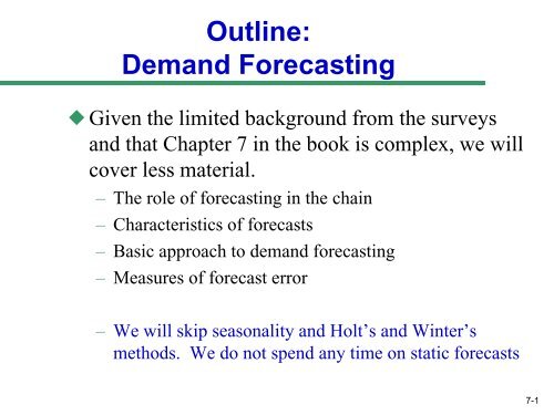
<strong>Outline</strong>:<br />
Demand Forecasting<br />
Given the limited background from the surveys<br />
and that Chapter 7 in the book is complex, we will<br />
cover less material.<br />
– The role of <strong>forecasting</strong> in the chain<br />
– Characteristics of forecasts<br />
– Basic approach to <strong>demand</strong> <strong>forecasting</strong><br />
– Measures of forecast error<br />
– We will skip seasonality and Holt’s and Winter’s<br />
methods. We do not spend any time on static forecasts<br />
7-1
Role of Forecasting<br />
in a Supply Chain<br />
The basis for all strategic and planning decisions<br />
in a supply chain<br />
Used for both push and pull processes<br />
Examples:<br />
– Production: scheduling, inventory, aggregate planning<br />
– Marketing: sales force allocation, promotions, new<br />
production introduction<br />
– Finance: plant/equipment investment, budgetary<br />
planning<br />
– Personnel: workforce planning, hiring, layoffs<br />
All of these decisions are interrelated<br />
7-2
Characteristics of Forecasts<br />
A FORECAST is a statement about the future<br />
– Absatzprognose, Vorhersage<br />
Forecasts are always wrong. Report both the expected<br />
value of the forecast and the measure of error<br />
Long-term forecasts are less accurate than short-term<br />
forecasts (forecast horizon is important)<br />
Aggregate forecasts are more accurate than disaggregate<br />
forecasts<br />
In order to forecast, the past has to have some relevance to<br />
the future<br />
7-3
Forecasting Methods<br />
Qualitative: primarily subjective; use judgment/opinion<br />
Time Series: use historical <strong>demand</strong> only<br />
– Static<br />
– Adaptive We will only consider adaptive<br />
Causal (or associative): use the relationship between <strong>demand</strong> and a<br />
factor other than pure time to develop forecast<br />
Simulation<br />
– Imitate consumer choices that give rise to <strong>demand</strong><br />
– Can combine time series and causal methods<br />
7-4
Basic Approach to<br />
Demand Forecasting<br />
Understand the objectives of <strong>forecasting</strong><br />
Integrate <strong>demand</strong> planning and <strong>forecasting</strong><br />
Identify major factors that influence the <strong>demand</strong><br />
forecast<br />
Understand and identify customer segments<br />
Determine the appropriate <strong>forecasting</strong> technique<br />
Establish performance and error measures for the<br />
forecast<br />
7-5
Components of an Observation<br />
Observed <strong>demand</strong> (O) =<br />
Systematic component (S) + Random component (R)<br />
Level (current deseasonalized <strong>demand</strong>)<br />
Trend (growth or decline in <strong>demand</strong>)<br />
Seasonality (predictable seasonal fluctuation)<br />
• Systematic component: Expected value of <strong>demand</strong><br />
• Random component: The part of the forecast that deviates<br />
from the systematic component<br />
• Forecast error: difference between forecast and actual <strong>demand</strong><br />
7-6
Steps in the Forecasting Process<br />
Step 1 Determine the purpose of forecast<br />
Step 2 Pick an appropriate time horizon<br />
Step 3 Select a <strong>forecasting</strong> technique<br />
- Plotting data may reveal patterns<br />
Step 4 Gather and analyze data in detail<br />
– State assumptions<br />
– Validate Data: May need to cleanse or filter for past events<br />
Step 5 Calculate forecast<br />
Step 6 Analyze/Monitor the forecast- Measure Accuracy<br />
Are results acceptable?<br />
No: Return to Step 3, revising forecast technique<br />
Yes: Publish forecast<br />
For ongoing <strong>forecasting</strong>: repeat Steps 4 through 6<br />
7
Time Series Forecasts<br />
Trend - long-term movement in data<br />
– Linear: steady increase (or decrease) over time<br />
– Not all trends are linear. Demand may be exponential, may both<br />
increase and decrease over product life cycle: VHS players<br />
Seasonality - short-term regular variations in data<br />
– Example: Walgreen’s sales of cold medications over the year<br />
– Not just limited to Fall/Winter/Spring/Summer variations<br />
» Weekly <strong>demand</strong> for reservations at expensive restaurants<br />
» Daily cycle of coffee sales at Starbucks<br />
Irregular variations - caused by unusual circumstances<br />
– Infrequent spikes<br />
– i.e. a stock market crash, 9/11 catastrophe<br />
Random variations - caused by chance
Time Series Forecasting<br />
Techniques Covered in this Class<br />
Averaging (or Smoothing)<br />
– Moving Average<br />
– Weighted Moving Average<br />
– Exponential Smoothing<br />
- Trend-Adjusted Exponential Smoothing (Holt’s) is not<br />
covered, nor is Winters (trend + seasonality)<br />
Linear Trend Analysis
Moving Average<br />
The average of the N most recent observations:<br />
MA<br />
n<br />
(<br />
t)<br />
t<br />
<br />
i t n<br />
1<br />
<br />
Example: a 4-period MA for time period 7 would be<br />
F 7= (A 6+A 5+A 4+A 3)/4<br />
The larger N, the smoother the forecast, but the greater the<br />
Lag (ability to respond to “real” changes)<br />
<br />
n<br />
A<br />
i<br />
10
General Note: To Write Formula<br />
with Respect to t or t+1<br />
Which is correct?<br />
1. F t+1 = (blah)A t + blah…<br />
2. F t = (blah)A t-1 + blah…<br />
Both are! As long as it’s clear just what t (or t+1) represents,<br />
these can be usable interchangeably<br />
– If you need to calculate the forecast for period 5, be clear<br />
whether t=5 or t+1=5<br />
But most important, don’t write:<br />
F t = (blah)A t + blah<br />
11
Weighted Moving Average<br />
Premise:The most recent observations might have the best<br />
predictive value. Yet for simple moving averages older data<br />
points have same importance as most recent<br />
We modify to give greater weight to more recent observations.<br />
(Remember: S W i = 1 or you get bias!)<br />
t 1<br />
it<br />
n<br />
WMAn(<br />
t)<br />
WiA<br />
Advantages: Avoids “oversmoothing” and lag time is<br />
decreased<br />
Weights are arbitrary, often found through trial and error!<br />
i<br />
12
Exponential Smoothing<br />
Exponential Smoothing is a type of Weighted Moving<br />
Average:<br />
F t = aA t-1 + a (1-a) A t-2 + a (1-a) 2 A t-3 + a (1-a) 3 A t-4+ ...<br />
However, it is much more easily written, computed and<br />
understood as:<br />
F a<br />
a<br />
t At<br />
1 ( 1<br />
) Ft<br />
<br />
Where a is between 0 and 1<br />
1<br />
13
More Exponential Smoothing<br />
Rearranging the terms shows this method can be viewed as the<br />
previous period’s forecast adjusted by a percentage of the<br />
previous period’s error (E t-1 = A t-1– F t-1)<br />
Ft F a<br />
A F<br />
t 1 ( t 1<br />
t 1<br />
The quickness of forecast adjustment is determined by the<br />
smoothing constant, a<br />
– The closer a to zero, the greater the smoothing<br />
– How do we pick a? Trial and error or can even optimize for it!<br />
– How to initialize the forecast? Many ways!<br />
» Book: average all the data we have so far<br />
» More practical and repeatable? Start it with F 2 = A 1<br />
)
How to Select a Forecast<br />
To forecast data without trends, we could use a simple naïve<br />
forecast, a MA (still need to pick the window), a WMA (need<br />
to pick both the window and the weights) or an exponential<br />
smoother (need to pick a)<br />
We will get many different answers- how do we pick the one<br />
we feel will have the best chance of being close to what will<br />
happen?<br />
We calculate past forecast accuracy, and we then pick the one<br />
that is most accurate.<br />
15
Measuring Forecast Accuracy<br />
•Error: difference between actual value and predicted value.<br />
Many different measures exist (we use MAD only)<br />
•Mean Absolute Deviation<br />
(MAD)<br />
• Mean Squared Error<br />
(MSE)<br />
• Standard Error<br />
(Standard Deviation)<br />
t<br />
<br />
MAD<br />
MSE<br />
t<br />
<br />
MSE<br />
t<br />
t<br />
<br />
i<br />
1<br />
t<br />
<br />
i1<br />
rule of thumbt<br />
<br />
t<br />
A<br />
A<br />
i<br />
t<br />
<br />
<br />
F<br />
i i<br />
t 1<br />
F<br />
1.<br />
25*<br />
i<br />
2<br />
MAD<br />
t
Linear Trend Analysis<br />
If there is a trend, the smoothing filters we have covered will<br />
LAG, resulting in bad forecasts.<br />
Plot the data first- in this example, do you see a trend?<br />
If the trend is linear, we will use Linear Trend Analysis<br />
– Caveat: Not all trends are linear! (We do not cover curvilinear regression in<br />
this class)<br />
sales<br />
180<br />
175<br />
170<br />
165<br />
160<br />
155<br />
150<br />
145<br />
sales by week<br />
0 2 4 6<br />
week
Y t = a + b*t<br />
Where<br />
a = intercept<br />
b = slope<br />
Linear Trend Equation<br />
185<br />
180<br />
175<br />
170<br />
165<br />
160<br />
155<br />
150<br />
145<br />
140<br />
1 2 3 4 5 6<br />
Looks like a simple line equation, but a and b are determined<br />
to minimize Mean Squared Error (MSE)
sales<br />
185<br />
180<br />
175<br />
170<br />
165<br />
160<br />
155<br />
150<br />
145<br />
Graphing the Results<br />
Regressing Sales Against Week<br />
1 2 3 4 5 6<br />
week<br />
Actual<br />
Forecast
Example:<br />
Linear Trend Analysis<br />
An intern at Netflix has been tracking weekly rentals of the<br />
direct-to-DVD movie “Barney Meets Vin_Diesel: Fossilized!”<br />
and, after noticing a pattern, has modeled them with a linear<br />
trend analysis. The Excel model gives a= 400, b= -10, where t<br />
= 0 was the DVD release week. It is currently week 12<br />
– What is the linear trend equation?<br />
– What are sales predicted to be this week?<br />
– What does the model predict sales will be a half year (26 weeks) after<br />
the release?<br />
– When does the model predict sales to stop? Do you believe this model is<br />
likely to be accurate for making long term predictions?
Associative Forecasting<br />
What if we think there is a better indicator of future behavior<br />
than time?<br />
Use explanatory or predictor variables to predict the future<br />
– E.g. Using interest rates to predict home purchases<br />
The associative technique used in this class is Simple Linear<br />
Regression<br />
– Linear Trend Analysis was an example where time t was used at the<br />
dependent variable. But now we can use factors other than time<br />
Y t = a + bt Linear Trend Analysis<br />
Y t = a + bX t Associative Forecast<br />
( X t is used instead of t)<br />
– Again, we use Excel to determine a and b
Associative Forecasting:<br />
Linear Regression<br />
Dependent variable<br />
Y<br />
Estimate of<br />
Y from<br />
regression<br />
equation<br />
Independent variable<br />
Actual<br />
value<br />
of Y<br />
Value of X used<br />
to estimate Y<br />
Regression<br />
equation:<br />
Y = a + bX<br />
X<br />
22
Associative Forecasting:<br />
Linear Regression<br />
Dependent variable<br />
Y Deviation,<br />
Estimate of or error<br />
Y from<br />
regression<br />
equation<br />
{<br />
Independent variable<br />
Actual<br />
value<br />
of Y<br />
Value of X used<br />
to estimate Y<br />
Regression<br />
equation:<br />
Y = a + bX<br />
X<br />
23
Example:<br />
Associative Forecast<br />
Sales Advertising<br />
Month (000 units) (000 $)<br />
1 264 2.5<br />
2 116 1.3<br />
3 165 1.4<br />
4 101 1.0<br />
5 209 2.0<br />
A rotor manufacturer has recorded these sales figures over the past 5<br />
months. They also know the budget spent promoting these parts<br />
1) Is there a = Y wide - bX variation in sales? b =<br />
2) Does this appear to be a good candidate for linear trend analysis?<br />
24
Now Consider Sales<br />
verses Advertising Spend<br />
25
How Strong is the Relationship?<br />
Correlation ( r ), measures strength and direction of the<br />
forecast of Y with respect to X (or t for linear trend analysis)<br />
– 0 < r
Example: Excel Solution<br />
to Linear Regression<br />
SUMMARY OUTPUT<br />
Regression Statistics<br />
Multiple R 0.979565<br />
R Square 0.959547<br />
Adjusted R Square 0.946063<br />
Standard Error 15.60274<br />
Observations 5<br />
ANOVA<br />
df SS MS F Significance F<br />
Regression 1 17323.66 17323.66 71.1604 0.0035<br />
Residual 3 730.3361 243.4454<br />
Total 4 18054<br />
Coefficients Standard Error t Stat P-valueLower 95%Upper 95% Lower 95.0% Upper 95.0%<br />
Intercept -8.13 22.35 -0.36 0.74 -79.27 63.00 -79.27 63.00<br />
X Variable 1 109.23 12.95 8.44 0.00 68.02 150.44 68.02 150.44<br />
27
Correlation is not Causation:<br />
An Example<br />
The following scatter-plot shows that the average life<br />
expectancy for a country is related to the number of doctors per<br />
person in that country. We could come up with all sorts of<br />
reasonable explanations justifying this, but…
Lurking Variables and Causation:<br />
Another Example<br />
This new scatter-plot shows that the average life expectancy for is<br />
also related to the number of televisions per person in that country.<br />
– And the relationship is even stronger: R 2 of 72% instead of 62%<br />
Since TVs are cheaper than doctors, Why don’t we send TVs to<br />
countries with low life expectancies in order to extend lifetimes.<br />
Right?
Lurking Variables and Causation:<br />
An Example<br />
How about considering a lurking variable? That<br />
makes more sense…<br />
– Countries with higher standards of living have both longer life<br />
expectancies and more doctors (and TVs!).<br />
– If higher living standards cause changes in these other variables,<br />
improving living standards might be expected to prolong lives and,<br />
incidentally, also increase the numbers of doctors and TVs.