Streamline Computation - FEFlow

DHI-WASY Streamline Computations Available in FEFLOW 1
Streamline Computations Available in FEFLOW
1 INTRODUCTION
H.-J. G. Diersch
DHI-WASY GmbH, Berlin
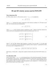
The evaluation of velocity fields is of important interest in the finite-element flow analysis. Commonly,
velocities are derived as nodal quantities from primary variables such as hydraulic head or
pressure by using suited projection (smoothing) techniques as described elsewhere 1,2,3 . If velocity
is known different evaluation methods are available to trace and visualize the flow field in postprocessing
procedures. The most general method concerns particle tracking 4 v h
p v
, where a pathline of an individual
fluid particle is traced in space x and time t via a Lagrangian approach. Particle tracking methods are
applicable in FEFLOW both in two dimensions (2D) and three dimensions (3D) under very general
flow conditions (presence of interior sinks/sources and/or boundary conditions such as pumping wells
and others). While they refers to individually moving particles which have to be appropriately assigned
at starting positions, a continuous picture of the overall flow movement is sometimes difficult to attain,
even if a large number of particles are traced.
There are efficient, but specific alternative methods for limited cases in 2D applications. These methods
represent streamline integrators, which facilitate the computation of flow pattern and distributed
discharge through the flow systems in a direct way. The theoretical basis of the two most important
streamline integrators, which are implemented in FEFLOW, will be described in the following.
2 PRELIMINARIES
We consider both Cartesian and cylindrical coordinate systems, such as
where x, y are Cartesian coordinates, z is vertical or axial coordinate, r is radial coordinate and ϑ is
azimuthal angle. The velocity vector v is accordingly defined as
The scalar product ∇ ⋅
v is given by
v
x
⎧x, y, z⎫
⎪ ⎪
= ⎨ x, y ⎬ for
⎪ ⎪
⎩r, ϑ, z⎭
⎧
⎪
⎪
⎪
⎪
u
v
w
= ⎨ for
⎪
⎪
⎪
⎪
⎩
v r
v ϑ
v z
⎧3D
⎪
⎨2D
⎪
⎩axisymmetry
Cartesian coordinates
cylindrical coordinates
(1)
(2)

DHI-WASY Streamline Computations Available in FEFLOW 2
( ∇ ⋅ v)
The vector cross-product ( ∇ × v)
reads
=
( ∇ × v)
∂u ∂v ∂w
----- + ----- + ------
∂x ∂y ∂z
∂u ∂v
----- + -----
∂x ∂y
1
--
r
∂ rv ( r)
1
-------------- --
∂r r
∂v ⎧
⎪
⎪
⎪
⎨
⎪
⎪
ϑ ∂vz ⎪ + ------- + ------
⎩
∂ϑ ∂z
=
⎧
⎪
⎪
⎪
⎪
⎪
⎪
⎪
⎪
⎪
⎪
⎪
⎪
⎨
⎪
⎪
⎪
⎪
⎪
⎪
⎪
⎪
⎪
⎪
⎪
⎪
⎩
∂w
------
∂y
∂u
-----
∂z
∂v
– -----
∂z
∂w
– ------
∂x
∂v ∂u
----- – -----
∂x ∂y
∂v
-----
∂x
3D (x, y, z) Cartesian
2D (x, y) Cartesian
cylindrical (r, ϑ, z)
In other notation ( ∇ ⋅ v)
is called the divergence of velocity vector v
0
0
∂u
– -----
∂y
1
--
r
∂vz ∂vϑ ------ – -------
∂ϑ ∂z
∂vz ∂vr ------ – ------
∂r ∂z
1
--
r
∂ rv ( ϑ)
1
--------------- --
∂r r
∂vr – ------
∂ϑ
div v = ∇ ⋅ v
3D (x, yz) , Cartesian
2D (x, y) Cartesian
cylindrical (r, ϑ, z)
and ( ∇ × v)
is called the curl of velocity vector v or the vorticity vector w
w = curl v = ∇ × v
From (4) is can be recognized that w in 3D represents a general vector field. Contrarily, in 2D and for
axisymmetric situations if assuming that all dependencies with respect to the azimuthal direction ϑ
vanish, i.e., vϑ = ∂⁄ ∂ϑ =
0 , we find the following useful curl-relations
(3)
(4)
(5)
(6)

DHI-WASY Streamline Computations Available in FEFLOW 3
where ω represents the (scalar) vorticity function.
3 STREAMLINES AND STREAMFUNCTION
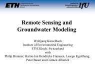
A streamline is the locus of points that are everywhere tangent to the instantaneous velocity vector v .
If ds is an element of length along a streamline, and thus tangent to the local velocity vector, then the
equation of a streamline is given by (Fig. 1)
or, in 2D Cartesian coordinates
⎧
⎪
∂v ∂u
----- – -----
⎪∂x
∂y
ω = w = ⎨
⎪∂v
z ∂vr ⎪------
– ------
∂r ∂z
⎩
Two streamlines cannot intersect except where v = 0 .
ds
ds × v = 0
dx
---u
=
2D (x, y) Cartesian
axisymmetric (r, z)
Since, by definition, no flow can cross a streamline it requires that the velocity vector field v have to
be divergence-free (solenoidal)
That means the flow is to be steady-state and no distributed sources and sinks can exist in the flow
domain.
An equation that would describe such streamlines in a 2D (and axisymmetric) flow may be written in
the form
dy----v
Figure 1 Definition of a streamline.
∇ ⋅ v = 0
ψ =
ψ( x, y)
v
ψ = const
(7)
(8)
(9)
(10)
(11)

DHI-WASY Streamline Computations Available in FEFLOW 4
where ψ is called the streamfunction. When ψ is constant (11) describes a streamline. It must obey the
general differential relation for the change in the streamfunction, dψ ,
The following definition relates ψ and the velocity components
for 2D and
dψ
for axisymmetric flow. The definitions (13) and (14) automatically satisfy the condition of free divergence
(10) in using (3). Substituting (13) into (12) it gives
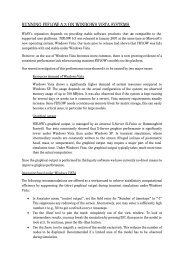
A major characteristic of the streamfunction is that the difference in ψ between two streamlines is
equal to the volume flow rate Q between those streamlines. Let us consider two streamlines with values
and as shown in Fig. 2.
ψ A
ψ B
The volume flow rate between the streamlines is
n
dy -dx
v r
v
=
∂ψ ∂ψ
------dx + ------dy
∂x ∂y
∂ψ
∂ψ
u = ------ v = – ------
∂y
∂x
1
--
r
∂ψ
1
= ------ vz --
∂z
r
∂ψ
= – ------
∂r
dψ = – v dx + u dy
ψ = ψ Β
ψ = ψ Α
Figure 2 Streamfunction in a plane flow.
Q AB
B
dy
= ∫v⋅n ds
=
∫(
unx + vny) ds
A
B
A
ds
n
-dx
n y
n x
(12)
(13)
(14)
(15)
(16)

DHI-WASY Streamline Computations Available in FEFLOW 5
where n is the normal unit vector. By geometry we have the relations nxds = dy and nyds = – dx
.
With these relations (16) becomes
The flow rate between streamlines is the difference in their streamfunction values. This equation is also
unaffected by the addition of an arbitrary constant to ψ .
4 STREAMLINE INTEGRATOR BY USING VORTICITY EQUATION
For 2D and axisymmetric flows a very efficient approach to computing the streamfunction distribution
for a given velocity field is based on using the vorticity function ω . By substituting the streamfunction
definition (13) into the vorticity equation (7) the following elliptic partial differential (Poisson) equation
is obtained
or
∇ 2
– ψ
B
∫
QAB = ( udy – vdx)
=
A
QAB = ψB – ψA ∇ 2 – ψ = ω
Equation (19) can be easily solved by the finite element method if formulating an unique boundary
value problem of the domain Ω enclosed by the boundary Γ . The Galerkin-based finite element formulation
of (19) gives (exemplified for 2D Cartesian)
∫
Ω
∇N∇N T ( dΩ)Y
by introducing finite element interpolation functions for the streamfunction and velocity components
where Y, U, V are nodal vectors and N are finite element shape functions. The boundary integral in
(20) vanishes because the flux normal to the streamline direction is zero,
n ⋅ ∇ψ
∂ψ ∂ψ
= nx------ + ny------ ∂x ∂y
= – nxv + nyu = 0 if the velocity vector field v is divergence-free (solenoidal),
i.e., ∇ ⋅ v =
0 . Accordingly, the following linear matrix system results
B
∫
A
dψ
⎧∂v
∂u 2D (x, y) Cartesian
⎪-----
– -----
⎪∂x
∂y
= ⎨
⎪⎛∂vz∂vr
------ – ------ ⎞raxisymmetric (r, z)
⎪⎝
∂r ∂z ⎠
⎩
=
∫
Ω
∂N T
---------V
∂x
∂NT
⎛ – ---------U ⎞dΩ+ Nn ( ⋅ ∇ψ)
⎝ ∂y ⎠ ∫ dΓ
ψ N T = Y
u N T = U
v N T = V
Γ
(17)
(18)
(19)
(20)
(21)

DHI-WASY Streamline Computations Available in FEFLOW 6
A ⋅ Y = BUV ( , )
for solving the streamfunction Y at each nodal point of a finite element mesh with known nodal velocity
components U, V.
The matrix A is symmetric and sparse. The equation system (22) is solved via
standard matrix solvers. However, a suitable boundary condition for Y is required. Practically, at only
one node on the outer boundary Γ the streamfunction is set to a Dirichlet-type reference value of zero.
The solution (22) is restricted to a solenoidal 2D (or axisymmetric) velocity vector field v , i.e., steadystate
flow, no interior boundary conditions (e.g., fluxes, wells) and absence of sinks and sources.
5 STREAMLINE INTEGRATOR BY USING BOUNDARY INTEGRAL
This streamline integration method is based on the numerically solution of differential (16) written in
the form
B
∫
δψ = ( unx + vny) ds
A
where δψ is the change in the streamfunction which is to be solved along a defined boundary. In the
preferred method the computation of δψ is carried out using (23) along each boundary of finite elements,
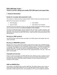
where the integration path AB is taken as element edge. We consider a typical element boundary
as shown in Fig. 3. The following finite element interpolations are introduced
u N T = U
v N T = V
x N T = X
y N T = Y
where N are finite element shape functions and U, V, X, Y are vectors of nodal point velocities and
coordinates.
y
global coordinates coordinate transformation local coordinates
x
Figure 3 Definition of element boundary for streamfunction computation.
In the finite element standard procedure the global coordinates ( x, y)
in 2D are transformed to local
coordinates ( ξ, η)
(Fig. 3). For a infinitesimal line element ds it results
ds
written for the local coordinate ( – 1 ≤ξ≤1) at element boundaries where η
sponds to the length of the boundary segment. Using (25) we find
= ± 1 . In (25) L
corre-
η
(-1,1) (1,1)
(-1,-1) (1,-1)
⎛∂x ----- ⎞
⎝∂ξ⎠ 2
⎛∂y ----- ⎞
⎝∂ξ⎠ 2
= + dξ = L dξ
ξ
element edge
(-1) n
(+1)
ξ
(22)
(23)
(24)
(25)

DHI-WASY Streamline Computations Available in FEFLOW 7
and their inverse
∂s
----- L
∂x
∂ξ
= -----
∂x
∂x
-----
∂s
1
--
L
∂x
-----
∂ξ
Using (27) the unit normal vector can be expressed by
n
=
∂s
----- L
∂y
∂ξ
= -----
∂y
Combining (25) and (28) with (23) the streamline integral along any finite element boundary takes the
form
δψ
=
where the coordinate interpolation functions (24) are applied.
The change in the streamfunction along any element edges is computed from (29) with known nodal
velocity vectors U, V.
The computation of the streamfunction for an entire finite element mesh is generated
by applying (29) along successive element boundaries, starting at a node for which a reference
value of ψ
has been specified. Unlike the vorticity integration method the present boundary integral
method is only an element-by-element procedure, which is computationally efficient and does not
require the solution of a matrix problem. However, the boundary integrator is also limited to solenoidal
velocity fields, i.e, steady-state flow, no interior boundary conditions (e.g., fluxes, wells) and absence
of sinks and sources.
6 CONCLUSIONS
FEFLOW provides two streamline integration methods (vorticity equation integrator and boundary
integral method) as additional tools to evaluate velocity fields in an alternative way in contrast to particle
tracking techniques. However, these streamline integrators are limited to steady-state 2D (or axisymmetric)
flow problems, where neither interior boundary conditions (such as fluxes or pumping
wells) nor sinks and sources should exist. While the boundary integral method does not require the
solution of a matrix problem, the vorticity equation integrator produces often more accurate results and
has shown more robust. Accordingly, the vorticity equation integrator represents the method of our
first choice. Streamline integrators are very useful for instance in density-variable flow simulations
(see 2D streamline patterns as shown in the references 1,2,3 ), where complex recirculating flow patterns
(eddies) can occur, which cannot be easily detected and visualized by using particle tracking methods.
In such cases, although the density-coupled mass (or heat) transport process is transient, the flow field
is divergence-free at each time step (FEFLOW runs in the so-called steady flow-transient transport
time mode) because the absence of storage (by fluid and skeleton compression) in the flow problem
assuming no interior boundary conditions and sinks/sources.
∂y
-----
∂s
∂y
n
----x
= =
∂s
=
ny ∂x
– -----
∂s
+1
∫
– 1
∂N T
=
1
--
L
1
--
L
∂y
-----
∂ξ
∂y
-----
∂ξ
∂x
– -----
∂ξ
---------Y N
∂ξ
T U ∂NT
---------X N
∂ξ
T ⎛ – V⎞dξ
⎝ ⎠
(26)
(27)
(28)
(29)

DHI-WASY Streamline Computations Available in FEFLOW 8
7 REFERENCES
1. Diersch, H.-J.G., Consistent velocity approximation in the finite-element simulation of density-dependent
mass and heat transport processes. FEFLOW’s White Papers Vol. I, Chapter 16, WASY GmbH, Berlin,
2002.
2. Diersch, H.-J.G., Coupled groundwater flow and transport: thermohaline and 3D convection systems.
FEFLOW’s White Papers Vol. I, Chapter 17, WASY GmbH, Berlin, 2002.
3. Diersch, H.-J.G., Variable-density flow and transport in porous media: approaches and challenges.
FEFLOW’s White Papers Vol. II, Chapter 1, WASY GmbH, Berlin, 2005.
4. Zheng, C. and Bennett, G.D. Applied contaminant transport modeling. Van Nostrand Reinhold, New York,
1995.