Using FEFLOW 6 (if you already know 5.x)
Using FEFLOW 6 (if you already know 5.x)
Using FEFLOW 6 (if you already know 5.x)

Create successful ePaper yourself
Turn your PDF publications into a flip-book with our unique Google optimized e-Paper software.
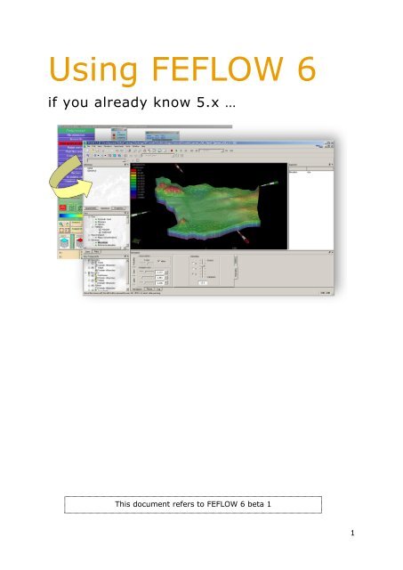
<strong>Using</strong> <strong>FEFLOW</strong> 6<br />
<strong>if</strong> <strong>you</strong> <strong>already</strong> <strong>know</strong> <strong>5.x</strong> …<br />
This document refers to <strong>FEFLOW</strong> 6 beta 1<br />
1
Table of Contents<br />
Preface ............................................................................................................... 5<br />
Welcome to <strong>FEFLOW</strong> 6 .................................................................................... 5<br />
Conventions and symbols in this reference ......................................................... 6<br />
The new workspace ............................................................................................ 7<br />
Menu commands ............................................................................................... 7<br />
Panels and toolbars ........................................................................................... 7<br />
Diagrams ......................................................................................................... 7<br />
Views .............................................................................................................. 7<br />
Supermesh view ............................................................................................ 8<br />
Slice view ...................................................................................................... 8<br />
3D view ........................................................................................................ 8<br />
Cross-section view ......................................................................................... 9<br />
A word on the philosophy of the new software ....................................................... 9<br />
Creating a new <strong>FEFLOW</strong> model ......................................................................... 11<br />
Maps ................................................................................................................. 11<br />
<strong>Using</strong> maps as a spatial reference ...................................................................... 11<br />
<strong>Using</strong> maps to import model properties .............................................................. 12<br />
Designing a supermesh .................................................................................... 13<br />
Navigation in the supermesh view ..................................................................... 13<br />
Manual supermesh design (digitizing maps) ........................................................ 13<br />
Snapping .................................................................................................... 13<br />
Polygon auto-completion ............................................................................... 14<br />
Importing lines, points and polygons from vector files .......................................... 14<br />
Splitting and joining polygons ........................................................................... 14<br />
Generating the finite-element mesh ................................................................. 15<br />
Choosing a mesh generator .............................................................................. 15<br />
Choosing the properties of a mesh generator ...................................................... 15<br />
Refinement .................................................................................................... 15<br />
Proposing element numbers .............................................................................. 16<br />
Generate automatically ................................................................................. 16<br />
Generate areally .......................................................................................... 16<br />
Generate gradually ....................................................................................... 16<br />
Problem settings .............................................................................................. 17<br />
2
Problem class and spec<strong>if</strong>ic option settings ........................................................... 17<br />
Temporal and control data ................................................................................ 17<br />
Time-varying functions (time series) .................................................................. 17<br />
Global settings ................................................................................................ 17<br />
Setting up a 3D model ...................................................................................... 18<br />
Viewing and mod<strong>if</strong>ying model properties ......................................................... 19<br />
Overview: the new workflow to edit model properties ........................................... 19<br />
Choosing model properties for visualization and data assignment ........................... 20<br />
Displaying model properties in the active view .................................................. 20<br />
Selecting a model property for data assignment ............................................... 20<br />
Restricting the visualization to a part of the model only ..................................... 20<br />
Initial conditions vs. process variables ............................................................. 20<br />
Creating selections of nodes or elements ............................................................ 21<br />
The d<strong>if</strong>ferent selection tools ........................................................................... 21<br />
Setting the snap distance for map selections .................................................... 22<br />
Copying selections to other slices or layers ...................................................... 22<br />
Storing and loading selections ........................................................................ 22<br />
Assigning data to a model property at a selection ................................................ 23<br />
Assigning constant values .............................................................................. 23<br />
Assigning time series .................................................................................... 23<br />
Importing constant values from maps ............................................................. 24<br />
Importing time series from maps .................................................................... 26<br />
The mesh inspector .......................................................................................... 28<br />
Data operations ................................................................................................ 29<br />
Deleting boundary conditions and constraints ...................................................... 29<br />
Copying data .................................................................................................. 29<br />
…to other properties ..................................................................................... 29<br />
…to other slices or layers ............................................................................... 29<br />
Import and export ........................................................................................... 30<br />
Importing boundary conditions and constraints ................................................. 30<br />
Exporting data as nodal or elemental values ..................................................... 30<br />
Exporting data plots ..................................................................................... 30<br />
Reference data ................................................................................................. 31<br />
Observation points .......................................................................................... 31<br />
Observation point groups ................................................................................. 31<br />
Cross sections (fences, segments, line sections) .................................................. 31<br />
Reference distributions ..................................................................................... 33<br />
Running the simulation .................................................................................... 34<br />
Saving DAC files .............................................................................................. 34<br />
3
Postprocessing ................................................................................................. 35<br />
Navigation in a .dac-file ................................................................................... 35<br />
Budgeting ...................................................................................................... 35<br />
Evaluating mass fluxes .................................................................................. 35<br />
Relating mass fluxes to nodes ........................................................................ 36<br />
Pathlines (particle tracking) .............................................................................. 37<br />
Outlook: <strong>FEFLOW</strong> functions not yet implemented ............................................. 41<br />
Features that will be available in a future release of <strong>FEFLOW</strong> 6 .............................. 41<br />
Time varying material parameters .................................................................. 41<br />
IFM modules ................................................................................................ 41<br />
Discrete feature elements .............................................................................. 41<br />
Multi-layer wells ........................................................................................... 41<br />
Borehole heat exchanger ............................................................................... 42<br />
Fluid flux analyzer ........................................................................................ 42<br />
Debug tool .................................................................................................. 42<br />
Parameter zones (<strong>FEFLOW</strong> Explorer) ............................................................... 42<br />
Converting data (conversion tool) ................................................................... 42<br />
Content analyzer .......................................................................................... 42<br />
Special operations ........................................................................................ 42<br />
Features that have been removed from <strong>FEFLOW</strong> .................................................. 42<br />
Mesh generator T-Mesh ................................................................................. 42<br />
4
Preface<br />
Welcome to <strong>FEFLOW</strong> 6<br />
With the release of <strong>FEFLOW</strong> 6, we have undertaken a complete refurbishment of<br />
the <strong>FEFLOW</strong> appearance. After using a UNIX-style Mot<strong>if</strong> GUI for almost 20 years,<br />
the time has come to create a friendlier, modern and most of all more productive<br />
type of user interface. The usage of hardware-accelerated 3D views, persistent<br />
links to data sources and many more features brings a lot of benefits to <strong>you</strong>, but<br />
also requires new workflows and ways to think when working with the new<br />
software.<br />
The first time <strong>you</strong> start <strong>FEFLOW</strong> 6 <strong>you</strong> might feel a bit uncomfortable. The green<br />
wallpapers have disappeared, being exchanged by grey parchment background;<br />
the blue menu buttons are gone and have been substituted by data trees.<br />
But <strong>you</strong> will soon see that working with the new <strong>FEFLOW</strong> is quick, intuitive, more<br />
transparent and fun! Some work steps are still very similar; and the ones that<br />
have been changed will be much easier to handle now.<br />
To remove the biggest obstacles on <strong>you</strong>r way to become a <strong>FEFLOW</strong> 6 expert, we<br />
have created this reference. It compares the important work steps in the old and<br />
the new <strong>FEFLOW</strong> interfaces and shows <strong>you</strong> how get <strong>you</strong>r work done efficiently. If<br />
<strong>you</strong> want to <strong>know</strong> the new features of the supermesh editor or how <strong>you</strong> can live<br />
without having a Join-operation, just go on with the next pages.<br />
All the best, <strong>you</strong>r <strong>FEFLOW</strong> team of DHI-WASY!<br />
5
Conventions and symbols in this reference<br />
In addition to the verbal description of the required screen actions we make use<br />
of some icons. They are intended to assist in relating the written description to<br />
the graphical information provided by <strong>FEFLOW</strong>. The icons refer to the kind of<br />
setting to be done:<br />
menu commands<br />
commands in the context menu<br />
(to be opened with the right mouse button)<br />
toolbars<br />
panels<br />
buttons in a dialog<br />
trees<br />
entries of trees<br />
input fields for text or numbers<br />
switch toggles<br />
radio buttons<br />
checkboxes<br />
6
The new workspace<br />
When <strong>you</strong> open <strong>FEFLOW</strong> 6 for the first time, <strong>you</strong> will notice that the developers<br />
have done more than just a transition of the old menu structure to a Windowsstyle<br />
platform.<br />
In <strong>FEFLOW</strong> <strong>5.x</strong> a static menu structure has been used, where <strong>you</strong> have been able<br />
to view and edit exactly one model property at a time at a fixed position in the<br />
program. <strong>FEFLOW</strong> 6 gives <strong>you</strong> more freedom: You are now able to display any<br />
combination of model properties at the same time, even while <strong>you</strong> are editing<br />
them.<br />
The tools to show and mod<strong>if</strong>y model properties are not hidden in menus<br />
anymore, but are accessible in toolbars and panels which are accessible at any<br />
time.<br />
The workspace (the <strong>FEFLOW</strong> window) is not static anymore, but can be changed<br />
and customized by the user. Panels and toolbars can be switched on and off, <strong>you</strong><br />
may also change their position in the workspace. They may even be placed<br />
outside the <strong>FEFLOW</strong> window, which is a handy feature <strong>if</strong> using more than one<br />
screen.<br />
To restore the original screen la<strong>you</strong>t, choose View > Reset Toolbar and<br />
Dock-window La<strong>you</strong>t from the menu. The next time <strong>FEFLOW</strong> 6 is started, the<br />
toolbars and panels will be re-arranged to their original state and position.<br />
Menu commands<br />
The menu is always visible and provides access the most important functions of<br />
<strong>FEFLOW</strong> 6.<br />
Panels and toolbars<br />
In contrast to the menu, panels and toolbars can be shown or hidden by using<br />
the menu command View > Panels and View > Toolbars, respectively.<br />
In this way, <strong>you</strong> can customize <strong>you</strong>r workspace the way <strong>you</strong> like it. You can also<br />
place panels and toolbars outside the <strong>FEFLOW</strong> window and on another screen.<br />
Diagrams<br />
Diagrams are special panels that usually display the development of a model<br />
property over space or time. They can be accessed using the menu entry<br />
View > Diagrams.<br />
Views<br />
Views are the primary windows where <strong>you</strong>r model is displayed and its properties<br />
can be mod<strong>if</strong>ied. There are four d<strong>if</strong>ferent types of views (Supermesh-, Slice-,<br />
7
3D- and Cross-section view), each providing a particular style to show the<br />
model and providing d<strong>if</strong>ferent tools depending on its particular purpose.<br />
Select View > Toolbars from the menu and choose the particular view from<br />
the list to create a new view.<br />
To navigate in the view, several tools are accessible in the View toolbar,<br />
whereas the behavior slightly changes with the type of view that is currently<br />
focused. Please see the description below.<br />
For more information on the various tools please refer to the respective parts of<br />
the help system.<br />
Supermesh view<br />
The Supermesh view will open when <strong>you</strong> start a new <strong>FEFLOW</strong> model. It is used<br />
to design the supermesh.<br />
Having focused this view, the necessary tools become available in the<br />
Supermesh menu and in the Supermesh toolbar.<br />
The recommended Navigation tool in the Supermesh view is the panning<br />
tool (hold down left mouse button to pan, hold down right mouse button to<br />
zoom).<br />
Slice view<br />
The Slice view is the direct FELOW 6 analog to the old working window in<br />
<strong>FEFLOW</strong> <strong>5.x</strong>. It provides a plan view of a single model slice of the finite element<br />
mesh.<br />
The recommended Navigation tool in the Slice view is the pan tool (hold<br />
down left mouse button to pan, hold down right mouse button to zoom)<br />
In a 3D model, <strong>you</strong> can browse the slices up and down using the and<br />
keys. Alternatively, <strong>you</strong> can directly choose a layer/slice from the<br />
Spatial Units panel.<br />
3D view<br />
The 3D view is available in 3D models only. If <strong>you</strong> are familiar with the <strong>FEFLOW</strong><br />
Explorer, <strong>you</strong> <strong>already</strong> <strong>know</strong> the principle of the navigation in this kind of window.<br />
Having the Rotate tool activated, <strong>you</strong> rotate the model around its centre of<br />
gravity by holding down the left mouse button; the location <strong>you</strong> catch with the<br />
mouse cursor will stick to the mouse cursors position. You cannot only grab parts<br />
of the model, but also other objects shown in the view like the handles.<br />
A small but useful new element is the auto-spinning behavior. Just rotate the<br />
model and release the left mouse button during the movement, the model will<br />
8
continue spinning around the last axis of rotation until <strong>you</strong> grab it again or hit<br />
.<br />
To pan the view to the left or the right, hold down the mouse wheel (center<br />
mouse button) and move the model in the chosen direction. Holding down the<br />
right mouse button activates zooming.<br />
In many cases, a model will have a rather small vertical extent compared to its<br />
horizontal dimensions. The (vertical) z-axis should be exaggerated in this case.<br />
This can be done in the Navigation panel. This panel contains all necessary<br />
functions to change the current view on the model. Click on the Distortion tab<br />
and sh<strong>if</strong>t the slider bar up until <strong>you</strong> have achieved a convenient view on the 3D<br />
model.<br />
Cross-section view<br />
Material properties and process variables can also be visualized in cross-section<br />
views.<br />
The area of a cross-section is defined as a line in the Slice view (called a 2D<br />
Surface line). Focus the Slice view and open its context menu (with the right<br />
mouse button). Choose Tools > Draw a 2D surface line.<br />
This line will be added to the Surface Locations section of the Spatial Units<br />
panel (The default name is 2D Polyline #...). Open the context menu of this line<br />
and choose Cross-Section view.<br />
A new Cross-Section view will open.<br />
A word on the philosophy of the new software<br />
As mentioned before, <strong>FEFLOW</strong> 6 gives the user a lot more freedom to choose<br />
<strong>you</strong>r own favorite workflow.<br />
In <strong>FEFLOW</strong> <strong>5.x</strong>, <strong>you</strong> worked <strong>you</strong>rself through the menus in a given order - from<br />
top to bottom.<br />
Within these menus, <strong>you</strong> followed a strict sequence of work steps again when<br />
assigning the model properties – first selecting the quantity, then inputing the<br />
value, and finally selecting the place where to apply it.<br />
9
In <strong>FEFLOW</strong> 6, the order of these steps is arbitrary. You may create a selection of<br />
nodes first, and then apply spec<strong>if</strong>ic values to d<strong>if</strong>ferent properties (e.g. a flow<br />
boundary condition and its respective constraint) afterwards. You can even store<br />
the selection for later use (for example to add a mass transport boundary<br />
condition when <strong>you</strong> extend the model at a later stage of <strong>you</strong>r project).<br />
Another aspect is the un<strong>if</strong>ication of tools in <strong>FEFLOW</strong> 6. For example, <strong>you</strong> have to<br />
learn and use only one single, powerful set of tools to create selections (instead<br />
of a slightly d<strong>if</strong>ferent tool for every single model property).<br />
This will allow the user to learn and use the software more efficiently, and will<br />
also be the basis for the development of more powerful features in the coming<br />
years.<br />
However, besides the changes during model property assignment, the overall<br />
workflow stays the same.<br />
You start with the design of a supermesh, usually based on background maps,<br />
that acts as the basis for the finite-elements mesh generation.<br />
Afterwards, <strong>you</strong> choose a model type in the problem settings and configure the<br />
3D layer setup.<br />
Next, the physical properties (initial condition, boundary conditions and material<br />
properties) are assigned to the model.<br />
Finally, <strong>you</strong> start the simulation, possibly storing the results in a DAC-file, which<br />
can be loaded for later post processing.<br />
The next chapters will guide <strong>you</strong> through these steps. If <strong>you</strong> need any help, do<br />
not hesitate to visit our web page or contact our support staff.<br />
10
Creating a new <strong>FEFLOW</strong> model<br />
By default, <strong>FEFLOW</strong> will <strong>already</strong> open an empty Supermesh when starting.<br />
If <strong>you</strong> have to start with a new model at a later stage, choose File > New to<br />
create a new model.<br />
Maps<br />
(Background-) Maps have two functions in a <strong>FEFLOW</strong> 6 model.<br />
<strong>Using</strong> maps as a spatial reference<br />
The first function is to provide the spatial reference<br />
to provide the geometry of the supermesh (either by manual digitizing or<br />
by direct import of polygons, lines and points).<br />
to create selections of nodes or elements (the former joining operation).<br />
to give the modeler a better orientation in general.<br />
<strong>Using</strong> background maps for these purposes is described in this chapter.<br />
All map-related operations are performed in the Maps panel,<br />
which carries over the functionality of the former Map-<br />
Manager.<br />
Initially, the list of registered maps is blank, except for a<br />
command Add Maps.... To add one or multiple maps to <strong>you</strong>r<br />
model, double click on this command or choose Add Map<br />
from the context menu in the Maps panel. A file selector will<br />
open that lets <strong>you</strong> choose one or multiple map files <strong>you</strong> want to load.<br />
Maps that have been registered to the fem-file in this way can be made visible in<br />
the current view window (for example the supermesh view). Perform a double<br />
click on the respective map in the Maps panel. In the case of vector data files<br />
(like ESRI shape files), a map contains one or more map layers. Map layers are<br />
used to define d<strong>if</strong>ferent views on the data of the same map. When a vector file is<br />
registered, a map layer Default is created automatically. Double click on the<br />
map layer instead of the map itself to make it visible in the active view.<br />
A general idea in <strong>FEFLOW</strong> 6 is the separation of the<br />
source of the data and the view on the data. The maps<br />
are an excellent example to explain this principle:<br />
The maps panel is a collection of all map data. It<br />
stores the location of the files and also the meaning of<br />
its data (physical unit, associated model property, etc).<br />
See section Importing constant values from maps for<br />
more information.<br />
11
On the contrary, the view on the data is controlled separately in the View<br />
Components panel.<br />
This panel contains a list of all visible items of the active view. The double click<br />
<strong>you</strong> performed on a map or map layer in the Maps panel before did nothing else<br />
then adding the map to the View Components panel.<br />
Note that the contents of the View Components panel always relate to the<br />
current active view window and changes when <strong>you</strong> activate another view.<br />
The maps, which are located in the Maps branch, can be switched on and off by<br />
activating or deactivating the checkbox in front of it. When <strong>you</strong> uncheck the<br />
checkbox of a complete branch, all of its contents become invisible at the same<br />
time. The layering order of the maps can be changed in a drag-and-drop<br />
manner as well.<br />
In case of vector maps, <strong>you</strong> may want to change the appearance of the enclosed<br />
point-, line- and polygon features. In the View Components panel, open the<br />
context menu of a map layer with the right mouse button and choose Edit<br />
Properties to open the Map Properties panel. Please refer to the help-system<br />
for detailed information.<br />
<strong>Using</strong> maps to import model properties<br />
A second aspect – and this is a new concept in <strong>FEFLOW</strong> 6 – is that all database<br />
files that are used for data import are handled as maps as well. <strong>Using</strong> Maps for<br />
this purpose will be described later in the section Importing constant values from<br />
maps.<br />
12
Designing a supermesh<br />
The Supermesh is an integral part of <strong>you</strong>r <strong>FEFLOW</strong> model now, which means that<br />
it will be saved in the .fem-file and will always be accessible even <strong>if</strong> <strong>you</strong> do not<br />
save it as a separate .smh-file (Even though this is still possible).<br />
The new supermesh editor gives <strong>you</strong> more than just better<br />
state-of-the-art graphics. The developers added a list of handy<br />
features to make the supermesh design more convenient and<br />
efficient. While creating polygons, lines and points, the new<br />
editor will make sure at any time that the supermesh geometry<br />
is valid to avoid time-consuming mistakes like overlapping<br />
polygons or gaps in the supermesh. If <strong>you</strong> need to change <strong>you</strong>r<br />
mesh later, <strong>you</strong> can split or merge existing polygons instead of<br />
having to delete and re-digitize the old ones.<br />
These tools (and of course the common tools <strong>you</strong> <strong>already</strong> <strong>know</strong><br />
from the <strong>FEFLOW</strong> <strong>5.x</strong> Mesh Editor) can be found in the<br />
Supermesh menu and in the Supermesh toolbar.<br />
Navigation in the supermesh view<br />
To pan the view (up/down/left/right), hold down the center<br />
mouse button (mouse wheel) and move the mouse in the<br />
respective direction. To change the zoom level (in/out), hold<br />
down the right mouse button and move the mouse up or<br />
down.<br />
Note that these navigation functions stay availble at any time, even while <strong>you</strong><br />
are currently drawing a line or polygon.<br />
Manual supermesh design (digitizing maps)<br />
Figure 2: The Supermesh toolbar<br />
Figure 1: Entries<br />
of the Supermesh<br />
Menu<br />
You can draw polygons, lines and points the way <strong>you</strong> are familiar with. If <strong>you</strong><br />
create a hole in the mesh (either accidently or by intention) it will be highlighted<br />
by a d<strong>if</strong>ferent color.<br />
Snapping<br />
All necessary tools can be found in the supermesh toolbar. Here, <strong>you</strong> also find<br />
the snapping functions. The handling is very similar to the <strong>5.x</strong> mesh editor:<br />
Choose a map (that has been added in the Maps panel before) from the drop<br />
down list and activate the Snap to point and/or Snap to line option.<br />
13
Polygon auto-completion<br />
Figure 3: Auto-completion<br />
of super elements<br />
The new auto-completion feature - that replaces the<br />
old key function from the <strong>5.x</strong> Mesh Editor -<br />
makes the creation of adjacent elements more<br />
convenient. When drawing along the boundary of an<br />
existing polygon, <strong>you</strong> do not have to click on every<br />
single node along the way anymore. Move the mouse<br />
cursor to a node on the border. The respective path<br />
with all its nodes will be highlighted and can be<br />
applied with a single click.<br />
Importing lines, points and polygons from vector files<br />
Alternatively, <strong>you</strong> can import points, lines and polygons directly from respective<br />
vector files. Register these files as maps in the Maps panel first. Afterwards, use<br />
the option Convert to... from the context menu of the map to create one or<br />
several supermesh features from the file.<br />
Note that the import of polygons is only possible <strong>if</strong> these polygons do not<br />
intersect with <strong>already</strong> existing polygons. Intersecting polygons are not imported.<br />
Splitting and joining polygons<br />
Completely new features in <strong>FEFLOW</strong> 6 are the Split<br />
Polygon and Join Polygons Tools. It is now possible<br />
to subdivide or join existing polygons without deleting them<br />
first. This makes the supermesh creation more intuitive, for<br />
<strong>you</strong> can digitize the outline of the model as one polygon at<br />
first, and split it up into sub-domains later.<br />
Figure 4: Subdividing<br />
a polygon with the<br />
split polygons<br />
function<br />
14
Generating the finite-element mesh<br />
Again, the workflow stays the same compared to <strong>FEFLOW</strong> <strong>5.x</strong>. After <strong>you</strong> have<br />
finished the supermesh, <strong>you</strong> create the finite element mesh using one of the<br />
available mesh generators directly from the Supermesh view by hitting the<br />
button of the toolbar.<br />
The Mesh Generator toolbar provides all necessary tools to control the mesh<br />
generation process.<br />
Figure 5: Mesh Generator toolbar<br />
Choosing a mesh generator<br />
For triangular meshes, the available mesh generators are Advancing Front,<br />
Gridbuilder and Triangle (TMesh has been removed as its application yields no<br />
additional benefits in almost every case nowadays). Choose the appropriate<br />
generator from the dropdown of the Mesh Generator toolbar.<br />
For quadrilateral meshes, Transport Mapping is available as an additional mesh<br />
generator. You can switch to a quadrilateral mesh by choosing Supermesh<br />
> Quadrilateral Mode from the menu. This should be done <strong>already</strong> when<br />
designing the supermesh (In this mode, the supermesh editor will make sure<br />
that only polygons with four edges are created).<br />
Choosing the properties of a mesh generator<br />
The generator properties can be accessed by hitting the button in the Mesh<br />
Generator toolbar. No sign<strong>if</strong>icant changes have been done in these dialogs since<br />
the <strong>5.x</strong> version.<br />
Refinement<br />
Refinement along polygon borders, lines or at points can be enabled in the<br />
Generator Properties. If <strong>you</strong> have chosen to refine only Selected lines or<br />
15
polygon borders, <strong>you</strong> need to spec<strong>if</strong>y these lines/borders in the supermesh<br />
editor:<br />
Push the Edge Selector button in the Mesh Generator toolbar. Select or<br />
deselect polygon borders or line sections by clicking directly on a line section or<br />
by drawing a rectangle around several line sections.<br />
Proposing element numbers<br />
Generate automatically<br />
In the easiest case, <strong>you</strong> just spec<strong>if</strong>y a target number of elements in the input<br />
field of the generator toolbar and hit the Generate Mesh button to start the<br />
generator.<br />
When the mesh generation is finished, a Slice view showing the generated mesh<br />
opens.<br />
Generate areally<br />
Very often it is required to propose a d<strong>if</strong>ferent number of elements per<br />
supermesh polygon. Hit the Edit Proposed Elements button in the<br />
Generator toolbar and click on the polygon for which <strong>you</strong> want to change the<br />
number of proposed elements.<br />
Alternatively, <strong>you</strong> can open the drop-down to choose a polygon from the list.<br />
Type the new value in the input field and press enter. The number is shown in<br />
red color to indicate that a custom value has been chosen.<br />
Continue with other polygons for which the number of elements should be<br />
proposed and hit the Generate Mesh button to generate the mesh with<br />
these settings.<br />
If <strong>you</strong> want to switch back to a globally proposed number, hit the Edit<br />
Proposed Elements button again. A warning message asks <strong>you</strong> <strong>if</strong> <strong>you</strong> want to<br />
reset the number of proposed elements. Confirm with Yes.<br />
Generate gradually<br />
This function has not been implemented, yet. It is planned for a future release of<br />
<strong>FEFLOW</strong>.<br />
16
Problem settings<br />
Figure 6: Accessing<br />
Problem Settings<br />
Figure 7: Problem<br />
Settings data tree.<br />
Problem class and spec<strong>if</strong>ic option settings<br />
As <strong>you</strong> <strong>know</strong>, <strong>FEFLOW</strong> includes a number of d<strong>if</strong>ferent<br />
numerical options to simulate flow and transport<br />
processes for d<strong>if</strong>ferent spatial dimensions (2D or 3D),<br />
temporal domains (steady-state or transient), projections<br />
(horizontal, vertical, axisymmetric), transport processes<br />
(single and multi-species, heat) and coupling processes<br />
(e.g. density dependency).<br />
In earlier <strong>FEFLOW</strong> versions, these properties had to be<br />
set at d<strong>if</strong>ferent locations (Problem Class, Temporal &<br />
Control Data and Spec<strong>if</strong>ic Options Settings). Now, all<br />
problem-related settings are consolidated in the<br />
Problem Settings dialog of the Edit Menu.<br />
The settings are sorted in a tree. The particular sections<br />
are thoroughly explained in the help system.<br />
Temporal and control data<br />
The settings of the former Temporal & Control data menu have been moved to<br />
the Temporal Properties and Numerical Settings section of the Problem<br />
Settings dialog.<br />
Time-varying functions (time series)<br />
The former Time-varying functions Editor can be accessed from the menu<br />
Edit > Time Series.<br />
Global settings<br />
Global Settings not related to an actual model like the number of threads used in<br />
parallel computing can be found in the Tools > Global Settings dialog.<br />
17
Setting up a 3D model<br />
If <strong>you</strong> <strong>know</strong> the 3D Layer Configurator from <strong>FEFLOW</strong> <strong>5.x</strong>,<br />
<strong>you</strong> will find the new dialog immediately familiar. It can be<br />
accessed from the menu Edit > 3D Layer<br />
Configuration.<br />
The design and the workflow of the 3D Layer configurator<br />
have been preserved.<br />
Figure 9: The 3D Layer Configurator<br />
Figure 8: Accessing<br />
the 3D Layer<br />
Configurator<br />
18
Viewing and mod<strong>if</strong>ying model properties<br />
Overview: the new workflow to edit model properties<br />
Back in <strong>FEFLOW</strong> <strong>5.x</strong>, the workflow to mod<strong>if</strong>y a model property included the<br />
following steps in the following order:<br />
1. Select a model property (from the respective <strong>FEFLOW</strong> menu).<br />
2. Enter a constant value, time function or select a database file.<br />
3. Select the nodes or elements where the constant value, time series or file<br />
data is to be applied to the model property.<br />
Basically, <strong>you</strong> will meet these exact steps in <strong>FEFLOW</strong> 6 again. But now, the<br />
workflow is more flexible as the order of these three working steps is arbitrary.<br />
The model properties - these are process<br />
variables, boundary conditions, material<br />
parameters and reference data - are accessible in<br />
a central place (the Data Panel). In this way, it<br />
is not necessary any more to navigate through<br />
lots of menus before a certain property can be<br />
displayed and edited.<br />
Values or time functions are chosen in the Editor<br />
toolbar, which is the new command central to<br />
select from the d<strong>if</strong>ferent types and sources.<br />
Manual input (Assign Values) is always<br />
available. If maps have been registered to the<br />
model or time series are defined, these options<br />
become available as well. A left click on the<br />
leading symbol in the dropdown lets <strong>you</strong> change<br />
the input method.<br />
Selections are the third requirement to assign<br />
data to a model property as any assignment is<br />
performed (only) on the current selection.<br />
The necessary tools to create a selection are<br />
available in the Selection toolbar. You will<br />
recognize some of the old tools from the <strong>5.x</strong><br />
version, but also new tools are available now.<br />
The former Joining method is integrated in this<br />
panel as well (except for the actual data<br />
assignment).<br />
The following sections describe these steps in<br />
detail.<br />
Figure 10: Data Panel<br />
Figure 11: Editor Toolbar<br />
Figure 12: Selection toolbar<br />
19
Choosing model properties for visualization and data assignment<br />
To make the available data more transparent and to allow the simultaneous<br />
visualization of d<strong>if</strong>ferent model properties, all properties have been consolidated<br />
in a single tree in the Data panel.<br />
Displaying model properties in the active view<br />
To plot a model property in the currently active View, perform a double click on<br />
that model property in the Data panel.<br />
To plot multiple data sources at the same time, hold down the -key while<br />
double clicking.<br />
The currently displayed data-sources are listed in the View Components panel.<br />
Selecting a model property for data assignment<br />
If only one model property is active, or – in the case of a multiple selection – the<br />
active properties are similar (like Kxx/Kyy/Kzz or In-Transfer Rate/Out-Transfer<br />
Rate), they are also open to data assignment.<br />
Be careful with multiple selections: If model properties are not similar,<br />
no assignment is possible.<br />
Restricting the visualization to a part of the model only<br />
In a 3D view, <strong>you</strong> can selectively plot data to a part of the model (e.g., a<br />
particular slice or layer). The available parts of the model are called spatial units<br />
and can be selected in the Spatial Units panel.<br />
By default, the data are displayed on the spatial unit Domain, the complete<br />
model. If <strong>you</strong> select another spatial unit here, a model property will be plotted to<br />
this unit exclusively when being activated in the Data Panel.<br />
For details on both View Components and Spatial Units panel, please refer to the<br />
<strong>FEFLOW</strong> Help System.<br />
IMPORTANT NOTE: When changing to a spatial unit other than Domain,<br />
make sure to switch back as soon as possible. It is very easy to forget<br />
that plotting is done only on a part of the model; and as a result <strong>you</strong><br />
might wonder why the data are not plotted even though <strong>you</strong> are double<br />
clicking on the correct entry in the data panel.<br />
Initial conditions vs. process variables<br />
The term “initial conditions” has been renamed to the more precise expression<br />
“process variables” (as the process variables only represent the initial conditions<br />
during the preprocessing; during the simulation run and postprocessing, these<br />
parameters represent modeling results instead).<br />
20
Creating selections of nodes or elements<br />
The Selection toolbar is the central place where all necessary tools to create a<br />
nodal or elemental selection can be found.<br />
Figure 13: The Selection toolbar<br />
A selection defines where a certain operation – including the assignment of data<br />
to a model property – is performed.<br />
Note: There are nodal and elemental selections. Wether a nodal or elemental<br />
selection is created depends on the model property that is currently active in the<br />
Data panel.<br />
A selection will not be cleared after the data assignment (as it was the case in<br />
<strong>FEFLOW</strong> <strong>5.x</strong>). In this way, <strong>you</strong> can use the same selection for the assignment of<br />
several related model properties (e.g., for a flow boundary condition and its<br />
related constraints) without the need to recreate it every time.<br />
However, it is recommended to clear a selection <strong>if</strong> it is not needed any more<br />
(otherwise it might accidently become part of a new selection created at a later<br />
point in time <strong>if</strong> <strong>you</strong> forget that it is still active).<br />
You can even store a selection permanently and re-use it at a later point in time.<br />
We encourage <strong>you</strong> to make use of this feature as often as possible, as it makes<br />
the work with <strong>FEFLOW</strong> much more productive, especially <strong>if</strong> <strong>you</strong> have to change<br />
model properties often, e.g. during calibration.<br />
The d<strong>if</strong>ferent selection tools<br />
All tools for manual and map-related selection of elements and nodes are<br />
available in the Selection toolbar. Open the dropdown list to choose from the<br />
available tools.<br />
When working in a Slice view, these are<br />
21
Select Individual Nodes/Elements (the former nodal/elemental<br />
selection)<br />
Select in Rectangular Region (the former rubberbox selection)<br />
Select using a Lasso (a new method to select in a free-hand region)<br />
Select in Polygonal Region (a new method to select in a polygon area to<br />
be drawn)<br />
Select in Polygonal Map Region (the former Joining Tool, only available<br />
<strong>if</strong> maps have been added to the model)<br />
Select Nodes Along a Border (the former border selection)<br />
When working in a 3D view, <strong>you</strong> can use the tool<br />
Select Complete Layer/Slice<br />
Please refer to the help system for more information.<br />
Setting the snap distance for map selections<br />
To change the snap distance, open Edit > Problem Settings. The Snap<br />
distance can be set in the Editor Properties section of this dialog.<br />
Copying selections to other slices or layers<br />
When working in a Slice view, the Copy Selection to Slices/Layers can<br />
be used to copy a selection from the current slice or layer to a number of other<br />
slices or layers. Note that nodes/elements on the target slice that are <strong>already</strong><br />
parts of the selection will not be removed from the selection.<br />
Storing and loading selections<br />
To store a selection for later use, open the Spatial Units panel and choose<br />
Store Current Selection from the context menu. This option is also available in<br />
the context menu of the Slice view and 3D view.<br />
To load a stored selection, choose Set as Current Selection from the context<br />
menu.<br />
Figure 14: Storing and loading selections in the Spatial Units panel<br />
22
Assigning data to a model property at a selection<br />
The assignment of data to any model property is usually performed on the<br />
current selection.<br />
There are four basic methods how model properties can be assigned:<br />
as constant values (Assign Values)<br />
as time series<br />
from a map (as constant values or as a time series)<br />
from a lookup table (as constant values)<br />
The input method is chosen in the Editor Toolbar. Here, <strong>you</strong> will also enter the<br />
respective value, or select a map or time function depending on the chosen<br />
method.<br />
The Editor toolbar is also the place where the data is finally applied by hitting<br />
Put Value button.<br />
In the Editor toolbar, <strong>you</strong> find a text input field. A symbol on the left indicates<br />
the currently selected assignment method:<br />
To change the input method, open the context menu of the symbol and choose<br />
another method from the list. Alternatively, <strong>you</strong> can cycle through the available<br />
methods clicking on the symbol with the left mouse button.<br />
Assigning constant values<br />
This approach relates to the former Assign tool (except for the database option)<br />
or Join tool (with constant option) in the <strong>5.x</strong> interface.<br />
Just enter a value in the text input field of the Editor toolbar (which replaces the<br />
Keyboard Request Box of the classic <strong>FEFLOW</strong>).<br />
The value is finally assigned to the selected model property at the current<br />
selection by hitting the Put Value button.<br />
Note: In <strong>FEFLOW</strong> 6 <strong>you</strong> can enter the value in any unit that is <strong>know</strong>n to <strong>FEFLOW</strong><br />
and part of the appropriate unit set. If <strong>you</strong> enter „1 ft“ to the Editor toolbar,<br />
<strong>FEFLOW</strong> will automatically convert the value to 0.3048 [m]. You can register<br />
<strong>you</strong>r own units or completely switch to another system of units (e.g. Imperial<br />
system) in the unit conversion dialog. See the help system for more<br />
information.<br />
Assigning time series<br />
When having defined at least one time series in the Time Series Editor, this<br />
method becomes available in the Editor toolbar.<br />
23
The Time Series Editor can be opened from the menu Edit > Time Series.<br />
Open the dropdown and choose the time series to be assigned.<br />
With <strong>you</strong> apply this time series to the active property on the active selected<br />
nodes or elements.<br />
The usage of time series is possible for boundary conditions at the moment. The<br />
values of time series must be based on the <strong>FEFLOW</strong> default as defined in Tools<br />
> Units….<br />
Importing constant values from maps<br />
Prerequisites to apply map data<br />
As the usage of GIS Data is the standard way to handle data for the major part<br />
of groundwater models, the import interfaces of <strong>FEFLOW</strong> have been further<br />
enhanced. The new features are more convenient to use, and also more<br />
powerful. The position of the GIS data files and its relation to the model’s data is<br />
maintained; this allows an easier update of the imported GIS data <strong>if</strong> the linked<br />
GIS files have become changed outside <strong>FEFLOW</strong>. With <strong>FEFLOW</strong> 6, <strong>you</strong> can<br />
therefore use a GIS system to completely control the data mod<strong>if</strong>ication,<br />
especially during the elaborate work of model calibration.<br />
These advances allow and require a better concept for the handling of the data<br />
than the one used in <strong>FEFLOW</strong> <strong>5.x</strong>. To guarantee consistency between d<strong>if</strong>ferent<br />
data sources, it is now obligatory to register the vector files by adding them as a<br />
background maps. For more information on how to load background maps, see<br />
chapter <strong>Using</strong> maps as a spatial reference.<br />
Vector and database files<br />
A data source usually consists of a vector file (.shp, .dxf or ASCII formats .pnt,<br />
.lin, .ply, etc) and a database file (.dbf, .dat, .trp). In some cases - e.g., .trp –<br />
the vector data is <strong>already</strong> part of the database file.<br />
The Maps panel is the command center where the association of data sources<br />
(including regionalization settings) to <strong>FEFLOW</strong> parameters is controlled. The work<br />
steps to assign Process Variables (initial conditions), boundary conditions and<br />
material properties have been un<strong>if</strong>ied.<br />
24
After a file with modeling data has been registered in the maps panel, only the<br />
position of the data files on the file system is <strong>know</strong>n to <strong>FEFLOW</strong>, but the meaning<br />
of the data is yet to be declared.<br />
To be able to import these values to the <strong>FEFLOW</strong> model, the contents of the<br />
fields must be associated with the corresponding model parameters. As the unit<br />
of the GIS data can be d<strong>if</strong>ferent from the <strong>FEFLOW</strong> units, a unit conversion might<br />
be necessary as well.<br />
In order to do this, open the context menu of the database file with a right click<br />
and choose Link to Parameter…. This will open the Parameter Association<br />
dialog.<br />
This dialog is mostly the one as <strong>you</strong> <strong>already</strong> <strong>know</strong> from <strong>FEFLOW</strong> <strong>5.x</strong>. From the<br />
list on the left (which contains the available fields of the database file) choose<br />
the field that contains the data to be imported. On the right, select the respective<br />
<strong>FEFLOW</strong> parameter and click on Add Link. Finally, choose the unit used in the<br />
data file from the dropdown list (the link turns red <strong>if</strong> a conversion is set).<br />
Figure 15: Selecting a database for the vector file<br />
Now, a link has been created and the data have been prepared for the final<br />
import.<br />
Regionalization of point data (formerly Assign Database)<br />
As <strong>you</strong> <strong>already</strong> <strong>know</strong> from <strong>FEFLOW</strong> <strong>5.x</strong>, point data is applied to the model<br />
through an appropriate regionalization method. In <strong>FEFLOW</strong> 6, the Regionalization<br />
method with all its settings has become a property of the data link.<br />
When working with point data soruces, the Parameter Association dialog provides<br />
an additional option Data regionalization method. It contains the options that<br />
<strong>you</strong> <strong>already</strong> <strong>know</strong> from the <strong>5.x</strong> Data regionalization menu. The new<br />
regionalization method Neighbourhood Relationship is a special option used to<br />
import solitary points data like the position of wells.<br />
25
Figure 16: Setting the properties of the data regionalization method<br />
Assignment of the data<br />
After <strong>you</strong> have prepared the data files and set the necessary units and<br />
regionalization settings, the actual assignment is only a very small step:<br />
Choose the Maps method in the editor toolbar and select the respective map<br />
from the dropdown.<br />
Alternatively, <strong>you</strong> can double click on any entry of the Linked attributes branch<br />
of any map (e.g. Value -> Elevation). This is a short cut to both select the<br />
correct map in the dropdown list of the Data panel and to activate the associated<br />
model property for data assignment.<br />
With a single click on the the data are imported from the map, eventually<br />
converted and interpolated, and finally assigned to the chosen model property at<br />
the current selection.<br />
Importing time series from maps<br />
To import time series IDs out of a map file, register this file as a map first. In the<br />
Parameter Association dialog, create a link to the respective model property<br />
and select the option Time-varying-power function ID.<br />
All other work steps are identical with the ones for importing constant values<br />
from a database file.<br />
26
The values from the database field are now interpreted as the IDs of time series<br />
as defined in the Time Series editor (choose from the menu Edit > Time<br />
Series).<br />
The usage of time series is possible for boundary conditions at the moment. The<br />
values of time series must be based on the <strong>FEFLOW</strong> default as defined in Tools<br />
> Units….<br />
27
The mesh inspector<br />
The good old mesh Inspector has survived this new major release.<br />
You can activate the Inspector using the Inspector button in the<br />
Inspection toolbar.<br />
Point the center of the Inspector’s magn<strong>if</strong>ying glass to an element or node to<br />
display the model properties currently visible in the active view window in the<br />
Inspector panel.<br />
Figure 17: Inspector panel<br />
Use the mouse wheel to change the zoom level (in/out) of the magn<strong>if</strong>ying glass<br />
(hold down the -key for a finer interval). You can adjust the size by<br />
holding down the -key while turning the mouse wheel.<br />
28
Data operations<br />
Deleting boundary conditions and constraints<br />
Deleting boundary conditions is quick and easy. Select the particular type of<br />
boundary condition or constraint for editing in the Data panel (double click) first.<br />
Press the Clear Value button of the Editor toolbar. All boundary conditions<br />
or constraints of the chosen type are deleted at the current selection.<br />
Copying data<br />
…to other properties<br />
In many cases, data must be transferred from one model property to another<br />
model property (e.g. from Conductivity [Kxx] to Conductivity [Kyy] and [Kzz]). In<br />
<strong>FEFLOW</strong> 6, this operation is done in a Copy & Paste manner.<br />
In order to transfer data from one model property to another,<br />
Create a selection in which the copying operation should be performed,<br />
e.g., all elements of a layer.<br />
Go to the Data panel.<br />
Double click on the source model property.<br />
Open the context menu of the source model property and choose Copy.<br />
Double click on the target model property.<br />
Open the context menu of the target model property and choose Paste.<br />
Within the current selection, the data are copied from the source model property<br />
to the target model property.<br />
…to other slices or layers<br />
To copy data of the same model property from a source slice/layer to a target<br />
slice/layer, the steps are slightly d<strong>if</strong>ferent. This option is only available in a Slice<br />
view.<br />
Open a Slice view.<br />
In the Data panel, double click on the source model property.<br />
In the Slice view, browse to the slice/layer from where <strong>you</strong> want to copy<br />
the data (source slice/layer) and create a selection.<br />
Open the context menu of the quantity <strong>you</strong> want to copy and choose<br />
Copy.<br />
Browse to the slice/layer where the data should be applied.<br />
In the Data panel, open the context menu of the model property <strong>you</strong> want<br />
to copy and choose Paste to Slice/Layer.<br />
Within the selection, the model property is now copied from the selection on the<br />
source slice/layer and transferred to a projection of the selection on the target<br />
slice/layer.<br />
29
Import and export<br />
Importing boundary conditions and constraints<br />
In <strong>FEFLOW</strong> <strong>5.x</strong>, the Assign-tool with Database option could be used import<br />
boundary conditions at solitary locations. In <strong>FEFLOW</strong> 6, this is done using the<br />
Neighborhood relationship regionalization method. This regionalization<br />
method reads point data from a file and applies it exclusively to the nearest node<br />
in the finite element mesh. This function allows a quick import of sparse data like<br />
boundary conditions.<br />
Add the file containing the boundary conditions coordinates and values (e.g., well<br />
coordinates and pumping rates) as a map in the Maps panel. Choose Link to<br />
Parameter from its context menu.<br />
In the Parameter Association dialog, link the value to the boundary condition<br />
and choose Neighborhood Relationship as a regionalization method.<br />
Assign the data using the Maps method of the Editor toolbar afterwards.<br />
Exporting data as nodal or elemental values<br />
In the Data panel, open the context menu of the model property <strong>you</strong> want to<br />
export. Choose Export Data … to write the nodal or elemental values to a file.<br />
Exporting data plots<br />
In the View Components panel, open the context menu of the model property<br />
<strong>you</strong> want to export. Choose Export Data … to write the nodal or elemental<br />
values to a file. You can choose from several styles that defining the way the<br />
data are exported. Please refer to the help system for further information.<br />
30
Reference data<br />
Observation points<br />
All operations concerning observation points can be accessed in the<br />
Observation Point Editor toolbar.<br />
Use the button to create observation points. If <strong>you</strong> place the mouse cursor<br />
near a node and create an observation point, it will automatically snap to this<br />
node. You can suppress snapping by holding down the key.<br />
The button creates a set of observation points from the current selection.<br />
The button deletes all observation points.<br />
To import observation points from a map, go to the map panel and choose<br />
Convert to > Observation Points from the maps context menu.<br />
Observation point groups<br />
This feature has not been implemented yet, but is planned for a future release of<br />
<strong>FEFLOW</strong>.<br />
Cross sections (fences, segments, line sections)<br />
The functions to plot material properties, layer geometry and process variables<br />
have <strong>already</strong> been available in <strong>FEFLOW</strong> <strong>5.x</strong>; but have been distributed around a<br />
number of d<strong>if</strong>ferent menus of the Reference Data and Postprocessor. In <strong>FEFLOW</strong><br />
6, the options and styles have been un<strong>if</strong>ied and two ways of displaying crosssections<br />
are available. Cross-sections can be plotted<br />
As a view component in a 3D view or<br />
As a cross-section view with the length of the fence as the x-axis and the<br />
geodetic elevation on the y-axis<br />
31
Figure 18: Cross-sections shown as view components in the 3D view (left) and in the<br />
cross-section view (right)<br />
Cross-sections can be created in the Slice view by using the Draw a Surface<br />
(2D) Line tool from the Tools section of the context menu (See Figure 19).<br />
Activate this tool and draw a line; a single click with the left mouse button sets a<br />
new point of the line, a double click sets the last point and finishes the line<br />
afterwards. You can cancel and line drawing by pressing the -button on<br />
<strong>you</strong>r keyboard.<br />
Figure 19: Creating a surface line in the 2D view<br />
Figure 20: Creating a<br />
Cross-section view from a<br />
2D Polyline<br />
The surface line is now available in the Surface Locations section of the Spatial<br />
Units panel. To display the cross-section as a vertical area in a 3D view, double<br />
click on the entry in the Spatial units (while the 3D view is the active window).<br />
32
A Cross-section view (see Figure 18) can be created by selecting Crosssection<br />
view from the 2D polylines context menu in the Spatial Units panel.<br />
Reference distributions<br />
Nodal and elemental reference distributions can be created directly in Reference<br />
data section of the Data panel.<br />
Open the context menu entry of the Reference Data branch and choose Add<br />
Nodal Reference Distribution or Add Elemental Reference Distribution.<br />
The reference distributions can be displayed and edited in the same way as any<br />
other data source.<br />
33
Running the simulation<br />
The sharp border between pre-processing, simulation and post processing has<br />
been overcome in <strong>FEFLOW</strong> 6. The simulator functions can now be accessed<br />
directly and at any time using the Simulatior toolbar.<br />
Figure 21: Simulation toolbar<br />
With a single click on the Run button the simulation is started. The<br />
Pause button will interrupt the simulation, while the Stop button<br />
terminates it. In case of transient simulations, the Simulator tool bar also<br />
displays the actual simulation time.<br />
Saving DAC files<br />
As in <strong>FEFLOW</strong> <strong>5.x</strong>, in order to save the intermediate results of the simulation,<br />
<strong>you</strong> need to select a results file where <strong>FEFLOW</strong> saves the data of particular time<br />
steps before starting the simulation. This can be done using the Record<br />
button of the simulator toolbar.<br />
Activate the checkmark before Save complete results (DAC file) and choose a<br />
file name. Exit the dialog with OK.<br />
Figure 22: Spec<strong>if</strong>ying a results file<br />
34
Postprocessing<br />
Navigation in a .dac-file<br />
Load a previously recorded dac-file from the<br />
Menu File > Open.<br />
Within the Simulator tool bar, <strong>you</strong> can browse<br />
forward or backward in time or<br />
directly select a time step from the drop-down menu.<br />
Budgeting<br />
The evaluation of water and mass fluxes at boundary conditions is a very<br />
important task during the Postprocessing. In our case, we are interested in the<br />
amount of contamination that is being infiltrated into the model area.<br />
Evaluation of mass fluxes<br />
Open the Budget panel from View > Panels > Budget Panel.<br />
There are separate budget analyses for the flow and for the transport model.<br />
Click on the Mass tab and check the Active checkbox to activate the budgeting<br />
(the budgeting is turned off by default as it can cause sign<strong>if</strong>icant computational<br />
effort).<br />
After a short computation time, the currently inflowing and outflowing mass is<br />
shown in the unit g/d, and is visualized as blue bars (in) and red bars (out).<br />
Initially, the budget is evaluated for the complete domain. To evaluate fluxes in a<br />
certain part of the model, a selection can be used to spec<strong>if</strong>y the respective nodes<br />
again.<br />
35
Create an arbitrary nodal selection (e.g., select all nodes along the southern<br />
boundary) and hit the Set Button. The budget result now shows mass flux in all<br />
selected nodes.<br />
Relating mass fluxes to nodes<br />
Choose Process Variables > Mass > Budget from the Data panel and activate<br />
it with a double click.<br />
At each node that is part of the current budget-selection, a colored sphere will<br />
appear in the 3D view. The color and size of the spheres indicate the amount of<br />
mass that is exchanged at this node.<br />
36
Pathlines (particle tracking)<br />
In <strong>FEFLOW</strong> <strong>5.x</strong>, the calculation of particle tracks in 2D and 3D has been done<br />
with d<strong>if</strong>ferent tools, each with a set of options for d<strong>if</strong>ferent purposes. In <strong>FEFLOW</strong><br />
6, these tools have been consolidated in one single workflow.<br />
Showing the trajectories of particles is done in the following steps:<br />
Define the starting location(s) of the pathlines<br />
Calculate the pathlines<br />
Set the properties of the trajectories<br />
Let us explain the whole procedure based on an example case, where the<br />
catchment area of a well gallery is to be delineated.<br />
At first, the locations (nodes) of the wells are selected.<br />
Afterwards, store the selection in the Spatial Units panel.<br />
Activate the selection in the Spatial Units panel (with a single left click) and<br />
switch to the Data panel. With a double Click on Process Variables > Flow ><br />
Pathlines (either backward or forward) <strong>you</strong> start the pathlines computation. The<br />
pathlines will be shown in the View Components panel and will be depicted in<br />
the active 2D or 3D view window.<br />
37
Figure 23: Plotting single pathlines for the Location Set<br />
You will see a single pathline evolving from each well. The seeds (starting points)<br />
of the pathlines are located directly on the wells. However, to delineate the<br />
catchment zones of the wells, we shall create a number of seeds on a circle<br />
around these wells. Since it would mean a much effort to create a location set for<br />
each of these circles manually, this functionality has now become a property of<br />
the pathlines themself. Choose Properties from the context menu of the<br />
Pathlines in the View Components panel. This opens the pathlines properties<br />
in the Properties panel.<br />
Figure 24: Delineation of the catchment of a well gallery by using pathlines swarms<br />
38
By choosing a Radius greater than zero, <strong>you</strong> invoke to create a pathlines swarm<br />
starting on a radius around the wells. The result is immediately shown in the<br />
currently active ciew (Figure 24 shows a 2D view). You can choose to create<br />
more or less seeds on the radius in the Seeds per Node tab.<br />
Note: If working with a 3D model, the pathline computation will always be done<br />
in three dimensions, even <strong>if</strong> working in the slice view (in this case, a projection<br />
to the slice is shown).<br />
Figure 25: Pathlines are plotted in a 3D view (red color). A group of 3rd kind boundary<br />
conditions representing a river is shown (green color).<br />
Besides creating seeds from a nodal selection (as described above), <strong>you</strong> also can<br />
also create them on arbitrary points in space, along lines or along polygons. The<br />
procedure is very similar. First <strong>you</strong> create a line or arbitrary point group as a<br />
Domain Location. In the 2D or 3D view, choose Tools from the context menu<br />
and select Draw a 3D Line or Draw a 3D point group, respectively. Create the<br />
line, polygon or point group by clicking on the fixed points on any surface. This<br />
can be a slice in the 2D view or any other surface on the 3D view, including<br />
cutting planes and cross-sections.<br />
Figure 26: Creating a 3D line<br />
39
Figure 27: Creating Pathlines from a 3D line<br />
40
Outlook: <strong>FEFLOW</strong> functions not yet implemented<br />
A few functions have not been implemented in the new Qt graphical user<br />
interface (GUI) of <strong>FEFLOW</strong> 6, yet. However, we are working hard to make them<br />
work in the near future. In some cases, <strong>you</strong> need to get back to the classic Mot<strong>if</strong><br />
GUI that is still available. If an alternative workaround is possible, <strong>you</strong> will find it<br />
here.<br />
Still, parameters that are assigned in the classic Mot<strong>if</strong> GUI will be fully regarded<br />
<strong>if</strong> a simulation runs in the <strong>FEFLOW</strong> 6 Qt GUI. If <strong>you</strong> plot the respective material<br />
parameters, <strong>you</strong> can even see the effects of these settings (for example timechanging<br />
material properties).<br />
Features that will be available in a future release of <strong>FEFLOW</strong> 6<br />
Time varying material parameters<br />
At the moment, the assignment of time-varying material parameters has to be<br />
done in the classic Mot<strong>if</strong> GUI of <strong>FEFLOW</strong>. Use the classic Mot<strong>if</strong> GUI of <strong>FEFLOW</strong> to<br />
define time-dependent materials.<br />
IFM modules<br />
The control panel of IFM modules has not been implemented in <strong>FEFLOW</strong>, yet, but<br />
is planned for a release in the near future. Use the classic Mot<strong>if</strong> GUI of <strong>FEFLOW</strong><br />
to add IFM modules to <strong>you</strong>r model.<br />
Discrete feature elements<br />
Discrete Feature Elements (DFE) are not implemented in <strong>FEFLOW</strong> 6, yet, but are<br />
planned for a release in the near future. Please use the classic GUI of <strong>FEFLOW</strong> to<br />
create DFE in <strong>you</strong>r model.<br />
<strong>FEFLOW</strong> 6 supports 3D-ESRI shape and 3D-DXF files as maps in the 3D view.<br />
You can use this functionality to visualize the position of fractures <strong>if</strong> this data is<br />
available.<br />
Multi-layer wells<br />
The Multi-layer well menu has not been implemented yet, but the functionality of<br />
the multi-layer well (well bore condition) is still regarded during the simulation.<br />
If <strong>you</strong> apply 4 th kind boundary conditions to the same node on adjacent slices,<br />
<strong>FEFLOW</strong> will connect these nodes by a high conductive element. Apply 4 th kind<br />
boundary conditions with a pumping rate of 0 m³/d to all nodes of the well<br />
screen, except for the bottommost node. Here <strong>you</strong> apply the total pumping rate<br />
of the screen.<br />
Alternatively, <strong>you</strong> can use the classic Mot<strong>if</strong> GUI to create the multi-layer wells.<br />
41
Borehole heat exchanger<br />
Borehole Heat Exchanger (BHE) have not been implemented in <strong>FEFLOW</strong> 6, yet,<br />
but are planned for a release in the near future. Please use the classic Mot<strong>if</strong> GUI<br />
of <strong>FEFLOW</strong> to assign BHE.<br />
Fluid flux analyzer<br />
The Fluid Flux analyzer has not been implemented in <strong>FEFLOW</strong> 6, yet. Please use<br />
the classic Mot<strong>if</strong> GUI of <strong>FEFLOW</strong>.<br />
Debug tool<br />
This feature has not been implemented yet, but is planned for a future release of<br />
<strong>FEFLOW</strong>. Please use the classic Mot<strong>if</strong> GUI of <strong>FEFLOW</strong>.<br />
Parameter zones (<strong>FEFLOW</strong> Explorer)<br />
This feature has not been implemented yet, but is planned for a future release of<br />
<strong>FEFLOW</strong>. Please use the <strong>FEFLOW</strong> Explorer instead.<br />
Converting data (conversion tool)<br />
This feature has not been implemented yet, but is planned for a future release of<br />
<strong>FEFLOW</strong>. Please use the classic Mot<strong>if</strong> GUI of <strong>FEFLOW</strong>.<br />
Content analyzer<br />
This feature has not been implemented, yet, but is planned for a future release<br />
of <strong>FEFLOW</strong>. Please use the classic Mot<strong>if</strong> GUI of <strong>FEFLOW</strong>.<br />
Special operations<br />
This feature has not been implemented, yet, but is planned for a future release<br />
of <strong>FEFLOW</strong>. Please use the classic Mot<strong>if</strong> GUI of <strong>FEFLOW</strong>.<br />
Features that have been removed from <strong>FEFLOW</strong><br />
Mesh generator T-Mesh<br />
T-Mesh has been removed from <strong>FEFLOW</strong>, as Gridbuilder and Triangle are much<br />
more powerful alternatives for complex geometries with Add-Ins.<br />
A re-implementation is not planned.<br />
42