Derivation of a Theoretically Maximum Evaporative Flux ... - FEFlow

WASY Theoretically maximum evaporative flux 1
Derivation of a Theoretically Maximum
Evaporative Flux Based on Gardner’s Analytical
Solution for an Unsaturated Soil Column
H.-J. G. Diersch
WASY Institute for Water Resources Planning and Systems Research Ltd., Berlin
ANALYTICAL SOLUTION IN THE VADOSE ZONE AT STEADY STATE
Assuming an exponential law for the relative conductivity as given by Gardner 1 and Philip 2
Kr( ψ)
which is related to the hydraulic conductivity according to
where is the sorptive number, the capillary pressure head and the saturated conductivity, an
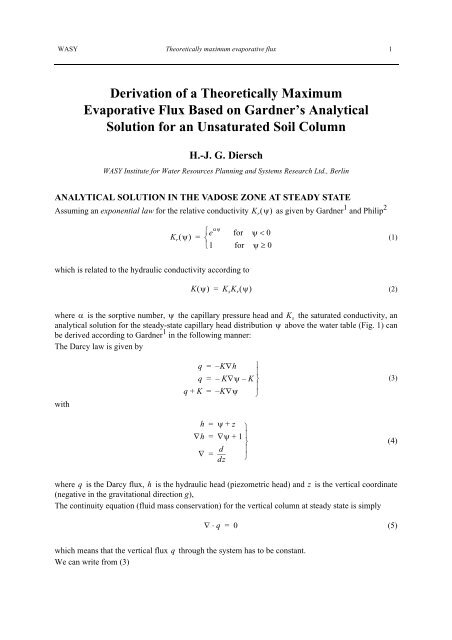
analytical solution for the steady-state capillary head distribution above the water table (Fig. 1) can
be derived according to Gardner 1 α ψ Ks ψ
in the following manner:
The Darcy law is given by
with
Kr( ψ)
e αψ ⎧ for ψ < 0
⎨
⎩1
for ψ ≥ 0
where q is the Darcy flux, h is the hydraulic head (piezometric head) and z is the vertical coordinate
(negative in the gravitational direction g),
The continuity equation (fluid mass conservation) for the vertical column at steady state is simply
which means that the vertical flux q
through the system has to be constant.
We can write from (3)
=
K( ψ)
= KsK r( ψ)
q = – K∇h
q = – K∇ψ – K
q+ K = – K∇ψ ⎭ ⎪⎬⎪⎫
h = ψ + z
∇h = ∇ψ + 1
∇
d
=
dz
⎭ ⎪⎬⎪⎫
∇ ⋅ q = 0
(1)
(2)
(3)
(4)
(5)

WASY Theoretically maximum evaporative flux 2
which can be integrated to obtain
or with (2) and (1)
Substituting
we get with
finally the solution as
dz( q + K)
= – Kdψ
∫dz
∫dz
=
=
vadose zone
water table
–
K
∫------------
dψ
q + K
Kse αψ
q Kse αψ
– ∫----------------------
dψ
+
Figure 1 Sketch of the unsaturated solution
domain above the water table.
v
a q Kse αψ
= +
a – q Kse αψ
=
da
-----dψ
αKse αψ
=
da αKse αψ = dψ
dψ
dψ
1
--------- e α
=
αK s
– ψ da
1
--
α
1
= -----------da
a– q
z
L
1
----------- =
a – q
e α – ψ
---------
Ks g
⎫
⎪
⎪
⎪
⎪
⎬
⎪
⎪
⎪
⎪
⎭
(6)
(7)
(8)
(9)
(10)

WASY Theoretically maximum evaporative flux 3
where ’ln’ represents the natural logarithm and C is an integration constant to be determined by the
following boundary conditions.
According to Fig. 1, where L is the depth of the water table and v is the evaporative flux (exfiltration
rate), we find from the continuity condition (5) that
Furthermore, we know that at z
Accordingly from (11) we obtain
= – L (the location of the water table) the pressure head ψ is zero.
Thus, with (12) and (13)
Since
it yields
and
1
∫dz
--
α
1
= – ∫--da
a
z = –
1
-- ln a + C
α
1
z -- ln q Kse α
αψ
⎫
⎪
⎪
⎪
⎬
⎪
⎪
= – + + C ⎪
⎭
– L
C
q = v
= –
1
-- ln q + Ks+ C ⎫
α
⎪
⎬
1
= -- ln q+ Ks– L ⎪
α
⎭
1
z --- ln v Kse α
αψ
= [ – + + ln v+ Ks] – L
1 v + Ks z --- ln
α v Kse αψ
⎫
⎪
⎪
⎬
= ⎛
⎝
----------------------
⎞ – L
⎪
+
⎠
⎪
⎭
v + Ks α( z + L)
ln
v Kse αψ
= ⎛
⎝
----------------------
⎞
+
⎠
e
+
v Kse αψ = ----------------------
+
α z L + ( ) v Ks v Kse αψ
+ ( v + Ks)e α – z L + ( )
=
αψ 1
e ---- ( v+ Ks)e Ks α – z L + ( )
= [ – v]
αψ ln 1
---- ( v + Ks)e Ks α – z L +
⎫
⎪
⎪
⎪
⎬
⎪
⎧ ( ) ⎫
= ⎨ [ – v]
⎪
⎬⎪
⎩ ⎭⎭
(11)
(12)
(13)
(14)
(15)
(16)
(17)

WASY Theoretically maximum evaporative flux 4
Finally, we find Gardner’s solution in the form
ψ( z)
1
-- ln e
α
α
– z L + ( ) v
Ks ⎛---- + 1⎞
v
– ----
⎝ ⎠
This solution can be used for either steady evaporation +v or infiltration – v.
TWO INTERESTING CASES RESULTUNG FROM EQ. (18)
Two interesting questions arise 3 :
(1) Which flux is concerned to force the pressure head ψ zero everywhere? From (18) we require
and can easily show that such a situation occurs if the infiltration has the amount of the saturated
conductivity
(2) Which flux is concerned to make the pressure head ψ infinity at the soil surface z = 0 ?
This should occur for a certain rate v which represents the theoretically maximum evaporative flux
.
v max
THE THEORETICALLY MAXIMUM EVAPORATIVE FLUX
The pressure head ψ becomes infinity at z
This implies that
= 0 if the argument of the logarithm of (18) goes to zero.
It gives a solution of the theoretically maximum evaporative flux as
where L
is the depth of the water table below the soil surface.
=
ln e α – z L + ( ) ⎛ v
---- + 1⎞
v
– ---- = 0
⎝ ⎠
K s
v = – Ks ψ( 0)
= ∞
vmax -------- e
Ks α
=
v max
– L vmax Ks K s
⎛-------- + 1⎞
⎝ ⎠
K s
e αL = ---------------
– 1
K s
v max
(18)
(19)
(20)
(21)
(22)
(23)

WASY Theoretically maximum evaporative flux 5
v max
EXAMPLES AND DISCUSSIONS REGARDING
We consider the behavior of vmax ⁄ Ks for a typical range of α-parameter,
e.g.,
α ( 12510 , , , ) m 1 –
=
Figure 2 illustrates the sharpness of the maximum evaporative flux in dependence on soil type α
and depth to the water table L . It points out the very rapid decrease in the evaporative flux as the depth
to the water table increases. Otherwise, the plots of Fig. 2 indicate that vmax tends to +∞ for small L
and to zero for large L .
v max /K s
v max /K s
10 0
10 -10
10 -20
10 -30
10 -40
10 -50
1000
900
800
700
600
500
400
300
200
100
0
α = 10 m -1
α = 5 m -1
v max
α = 2 m -1
α = 1 m -1
1 10 100
L [m]
10 -3 10 -2 10 -1 10 0 10 1 10 2
Figure 2 Maximum evaporative flux vmax ⁄ Ks in dependence on the depth to the water
table L and the soil parameter α .
αL
(24)

WASY Theoretically maximum evaporative flux 6
The maximum evaporative flux seems to be useful to limit the actual evaporation rate in a numerical
simulation, for instance, in such a way as
v max
where can be estimated by
in which, in contrast to the exact formula (23), the depth of the water table L is approximated by the
suction head ψ at the surface of the soil.
Alternatively, introducing the effective saturation
where s is the saturation and sris the residual saturation, we find for the exponential law the simple
capillary pressure-saturation relationship
It can be used to express directly the maximum evaporative flux as a function of the effective
saturation . Since
s e
we find from (26) after simple manipulations
REFERENCES
v actual
=
v max
min v prescribed ( , vmax) s e
K s
e αψ = ------------------
– 1
s e
s – sr = ------------
1 – sr se e αψ = for ψ < 0
s e
– ψ 1
e α
e αψ
= = ---------
v max
seK s
=
------------
1 – se
1. Gardner, W.R., Some steady-state solutions of the unsaturated moisture flow equation with application to
evaporation from a water table. Soil Sci. 35 (1958) 4, 228-232.
2. Philip, J.R., Theory of infiltration. Adv. Hydroscience 5 (1969), 215-296.
3. Selker, J.S., Keller, C.K. and McCord, J.T., Vadose zone processes. Lewis Publ., Boca Raton, 1999.
v max
(25)
(26)
(27)
(28)
(29)
(30)