Quanto Adjustments in the Presence of Stochastic Volatility
Quanto Adjustments in the Presence of Stochastic Volatility
Quanto Adjustments in the Presence of Stochastic Volatility

Create successful ePaper yourself
Turn your PDF publications into a flip-book with our unique Google optimized e-Paper software.
<strong>Quanto</strong> <strong>Adjustments</strong> <strong>in</strong> <strong>the</strong> <strong>Presence</strong> <strong>of</strong> <strong>Stochastic</strong> <strong>Volatility</strong> ∗<br />
Alexander Giese †<br />
March 14, 2012<br />
Abstract<br />
This paper considers <strong>the</strong> pric<strong>in</strong>g <strong>of</strong> quanto options <strong>in</strong> <strong>the</strong> presence <strong>of</strong> stochastic volatility. While it is wellknown<br />
that <strong>the</strong> quanto adjustment <strong>in</strong> <strong>the</strong> drift <strong>of</strong> <strong>the</strong> underly<strong>in</strong>g has a significant impact on <strong>the</strong> prices <strong>of</strong> quanto<br />
options, this paper po<strong>in</strong>ts out that an additional quanto adjustment <strong>in</strong> <strong>the</strong> underly<strong>in</strong>g’s volatility needs to be<br />
considered <strong>in</strong> <strong>the</strong> presence <strong>of</strong> stochastic volatility. By deriv<strong>in</strong>g closed-form solutions for standard quanto options,<br />
<strong>the</strong> paper demonstrates that this additional quanto adjustment also has a material impact on quanto options.<br />
Fur<strong>the</strong>rmore, numerical examples are presented toge<strong>the</strong>r with a comparison <strong>of</strong> <strong>the</strong> proposed model aga<strong>in</strong>st three<br />
commonly used standard pric<strong>in</strong>g methods for quanto options.<br />
∗ The paper has been accepted for publication by <strong>the</strong> Risk magaz<strong>in</strong>e.<br />
† UniCredit, Quantitative Product Group, Arabellastrasse 12, D-81925 Munich (alexander.giese@unicreditgroup.de)<br />
1
1 Introduction<br />
<strong>Quanto</strong> options are options where <strong>the</strong> pay<strong>of</strong>f is paid <strong>in</strong> a currency different from <strong>the</strong> currency <strong>in</strong> which <strong>the</strong> underly<strong>in</strong>g<br />
asset is traded and where <strong>the</strong> applied foreign exchange (FX) rate between <strong>the</strong> two currencies is set to one.<br />
The fixed FX rate allows <strong>the</strong> holder <strong>of</strong> a quanto option to participate on <strong>the</strong> performance <strong>of</strong> <strong>the</strong> underly<strong>in</strong>g without<br />
carry<strong>in</strong>g <strong>the</strong> risk <strong>of</strong> a chang<strong>in</strong>g FX rate. For <strong>in</strong>stance for a Euro-based <strong>in</strong>vestor who is seek<strong>in</strong>g option exposure on<br />
<strong>the</strong> S&P 500 but does not want to be exposed to changes <strong>of</strong> <strong>the</strong> Euro/US Dollar exchange rate, a quanto option on<br />
<strong>the</strong> S&P 500 is a very suitable f<strong>in</strong>ancial product as it pays <strong>the</strong> pay<strong>of</strong>f <strong>of</strong> a standard non-quanto option on <strong>the</strong> S&P<br />
500 and converts <strong>the</strong> payout with a guaranteed rate <strong>of</strong> 1 from US Dollar <strong>in</strong>to Euro at maturity. <strong>Quanto</strong> options are<br />
traded as over-<strong>the</strong>-counter (OTC) contracts and are also <strong>of</strong>ten embedded <strong>in</strong> structured equity products <strong>of</strong>fered to<br />
end <strong>in</strong>vestors due to <strong>the</strong> <strong>in</strong>creas<strong>in</strong>g globalization <strong>of</strong> equity <strong>in</strong>vestments.<br />
The pric<strong>in</strong>g and risk management <strong>of</strong> quanto options on foreign equities have become <strong>in</strong>creas<strong>in</strong>gly challeng<strong>in</strong>g <strong>in</strong><br />
<strong>the</strong> past years due to unpredicted levels <strong>of</strong> <strong>the</strong> equity/FX correlations and high volatilities. Both market parameters<br />
determ<strong>in</strong>e <strong>the</strong> well-known quanto adjustment <strong>in</strong> <strong>the</strong> drift <strong>of</strong> <strong>the</strong> underly<strong>in</strong>g as derived by Re<strong>in</strong>er [8] <strong>in</strong> <strong>the</strong> classical<br />
Black-Scholes model. While most <strong>of</strong> <strong>the</strong> research on quanto options has focused on <strong>the</strong> Black-Scholes framework,<br />
researchers recently started to study quanto options <strong>in</strong> <strong>the</strong> context <strong>of</strong> stochastic volatility models which allow to <strong>in</strong>corporate<br />
skews and smiles <strong>in</strong> <strong>the</strong> implied volatility surface <strong>of</strong> <strong>the</strong> underly<strong>in</strong>g asset. Dimitr<strong>of</strong>f et al. [1] assume <strong>the</strong><br />
Heston [3] model and Jäckel [5] uses a stochastic local volatility model <strong>in</strong> <strong>the</strong>ir studies on quanto options. While<br />
both studies conclude that <strong>the</strong> quanto option prices <strong>in</strong> a stochastic volatility model differ from <strong>the</strong> correspond<strong>in</strong>g<br />
prices obta<strong>in</strong>ed by apply<strong>in</strong>g standard pric<strong>in</strong>g methods, <strong>the</strong>y provide little explanation and <strong>in</strong>tuition for <strong>the</strong> observed<br />
price differences. Fur<strong>the</strong>rmore, <strong>in</strong> both papers <strong>the</strong> model prices for quanto options needed to be calculated us<strong>in</strong>g<br />
ei<strong>the</strong>r Monte Carlo methods or numerical solutions <strong>of</strong> <strong>the</strong> pric<strong>in</strong>g PDE due to <strong>the</strong> absence <strong>of</strong> closed-form solutions.<br />
Motivated by <strong>the</strong>se recent numerical studies <strong>of</strong> quanto options <strong>in</strong> <strong>the</strong> presence <strong>of</strong> stochastic volatility, we aim to<br />
obta<strong>in</strong> closed-form solutions for standard quanto options under <strong>the</strong> assumption <strong>of</strong> a stochastic volatility model for<br />
<strong>the</strong> underly<strong>in</strong>g asset <strong>in</strong> order to facilitate fast and efficient pric<strong>in</strong>g and risk management <strong>of</strong> <strong>the</strong>se options. We also<br />
try to provide a good understand<strong>in</strong>g and <strong>in</strong>tuition for <strong>the</strong> ma<strong>in</strong> factor caus<strong>in</strong>g <strong>the</strong> price differences between <strong>the</strong><br />
quanto option prices obta<strong>in</strong>ed us<strong>in</strong>g <strong>the</strong> derived pric<strong>in</strong>g formulas and <strong>the</strong> option prices obta<strong>in</strong>ed by us<strong>in</strong>g standard<br />
pric<strong>in</strong>g methods for quanto options.<br />
The rema<strong>in</strong>der <strong>of</strong> this paper is organized as follows. We first <strong>in</strong>troduce <strong>the</strong> stochastic volatility model and derive<br />
closed-form solutions for <strong>the</strong> quanto forward <strong>in</strong> <strong>the</strong> model framework. Closed-form solutions for standard quanto<br />
options are derived <strong>in</strong> Section 3 which represents <strong>the</strong> ma<strong>in</strong> result <strong>of</strong> <strong>the</strong> paper. Afterwards, Section 4 discusses<br />
<strong>the</strong> calibration <strong>of</strong> <strong>the</strong> model and analyzes <strong>the</strong> impact <strong>of</strong> an additional quanto adjustment which we identify to be<br />
present. Section 5 presents numerical examples where <strong>the</strong> model prices are compared aga<strong>in</strong>st three commonly<br />
used pric<strong>in</strong>g methods for quanto options. Fur<strong>the</strong>rmore, a numerical example for <strong>the</strong> impact <strong>of</strong> <strong>the</strong> implied volatility<br />
skew <strong>of</strong> foreign exchange options on <strong>the</strong> prices <strong>of</strong> quanto options is given. F<strong>in</strong>ally, Section 6 concludes <strong>the</strong><br />
paper.<br />
2 The model<br />
The price process <strong>of</strong> <strong>the</strong> underly<strong>in</strong>g S is assumed to be denom<strong>in</strong>ated <strong>in</strong> <strong>the</strong> foreign currency X and to follow <strong>the</strong><br />
dynamics:<br />
dS(t) = (r X − d)S(t)dt + ν(t)S(t)dW QX<br />
S (t), S(0) = S0, (1)<br />
dν(t) = κ (θ − ν(t)) dt + δdW QX<br />
ν (t), ν(0) = ν0, (2)<br />
under <strong>the</strong> foreign risk-neutral measure QX where W QX<br />
S and W QX<br />
ν are two Brownian motions, rX is <strong>the</strong> foreign<br />
<strong>in</strong>terest rate, d is <strong>the</strong> dividend yield and ν is <strong>the</strong> stochastic volatility process <strong>of</strong> <strong>the</strong> underly<strong>in</strong>g S with <strong>the</strong> constant<br />
parameters κ (mean reversion speed), θ (long-term mean volatility) and δ (volatility <strong>of</strong> volatility). Here we assume<br />
<strong>the</strong> stochastic volatility model <strong>of</strong> Schöbel and Zhu [9] for <strong>the</strong> underly<strong>in</strong>g price process where <strong>the</strong> volatility ν<br />
follows an Ornste<strong>in</strong>-Uhlenbeck process. This model choice will allow us later to derive closed-form solutions for<br />
standard quanto options, however, we strongly believe that most <strong>of</strong> <strong>the</strong> observations and conclusions <strong>of</strong> this paper<br />
apply to stochastic volatility models <strong>in</strong> general. 1<br />
1 The Schöbel and Zhu [9] model has <strong>of</strong>ten been criticized for allow<strong>in</strong>g <strong>the</strong> <strong>in</strong>stantaneous volatility ν to becom<strong>in</strong>g negative. However, this<br />
does not pose any ma<strong>the</strong>matical or numerical problem as <strong>the</strong> non-negativity constra<strong>in</strong>t only needs to be imposed on <strong>the</strong> variance ra<strong>the</strong>r than <strong>the</strong><br />
2
Fur<strong>the</strong>rmore, we assume an <strong>in</strong>vestor whose domestic currency is Y and who wishes to obta<strong>in</strong> exposure to <strong>the</strong><br />
underly<strong>in</strong>g S without carry<strong>in</strong>g FX risk. Let Z Y/X denote <strong>the</strong> foreign exchange rate (price <strong>of</strong> one unit <strong>of</strong> currency<br />
Y <strong>in</strong> units <strong>of</strong> currency X) and we assume Z Y/X is given by Black-Scholes model dynamics under Q X :<br />
dZ Y/X (t) = (r X − r Y )Z Y/X (t)dt + σF XZ Y/X (t)dW QX<br />
Z (t), ZY/X (0) = Z Y/X<br />
0<br />
where W QX<br />
Z is a Brownian motion, rY is <strong>the</strong> domestic <strong>in</strong>terest rate and σF X is <strong>the</strong> constant volatility <strong>of</strong> <strong>the</strong> FX<br />
rate process ZY/X . The model allows for constant correlations between all driv<strong>in</strong>g factors, i.e. 2<br />
�<br />
d W QX<br />
�<br />
�<br />
QX<br />
S , Wν (t) = ρS,νdt, d W QX<br />
�<br />
�<br />
QX<br />
S , WZ (t) = ρS,Zdt, d W QX<br />
ν , W QX<br />
�<br />
Z (t) = ρν,Zdt.<br />
After a change <strong>of</strong> measure from QX to <strong>the</strong> <strong>the</strong> domestic risk-neutral measure QY with<br />
QY QX �<br />
�<br />
�<br />
� =<br />
Ft<br />
ZY/X (t)<br />
ZY/X (0) e(rY −r X )t −<br />
= e 1<br />
2 σ2<br />
F X t+σF X W QX<br />
Z (t) ,<br />
Girsanov’s <strong>the</strong>orem implies that <strong>the</strong> processes W QY<br />
S , W QY<br />
ν and W QY<br />
F X def<strong>in</strong>ed by<br />
dW QY<br />
S (t) = dW QX<br />
S (t) − ρS,ZσF Xdt,<br />
dW QY<br />
ν (t) = dW QX<br />
ν (t) − ρν,ZσF Xdt,<br />
dW QY<br />
QX<br />
F X (t) = −dWZ (t) + σF Xdt,<br />
are Brownian motions under <strong>the</strong> domestic measure Q Y . The measure Q Y is also <strong>of</strong>ten referred to as <strong>the</strong> quanto<br />
measure. One obta<strong>in</strong>s <strong>the</strong> follow<strong>in</strong>g dynamics <strong>of</strong> <strong>the</strong> processes S and v under Q Y :<br />
dS(t) = (r X − d − ρS,F XσF Xν(t))S(t)dt + ν(t)S(t)dW QY<br />
S (t), (3)<br />
dν(t) = [κ(θ − ν(t)) − ρν,F XσF Xδ] dt + δdW QY<br />
ν (t),<br />
= κ( ˆ θ − ν(t))dt + δdW QY<br />
ν (t), (4)<br />
dZ X/Y (t) = (r Y − r X )Z X/Y (t)dt + σF XZ X/Y (t)dW QY<br />
F X (t),<br />
with ˆ θ = θ − ρν,F X σF X δ<br />
κ , ρS,F X = −ρS,Z, ρν,F X = −ρν,Z and <strong>the</strong> FX rate ZX/Y denot<strong>in</strong>g <strong>the</strong> price <strong>of</strong> one unit<br />
<strong>of</strong> currency X <strong>in</strong> units <strong>of</strong> domestic currency Y � ZX/Y (t) = 1/Z Y/X (t) � . Fur<strong>the</strong>rmore, <strong>the</strong> correlation matrix<br />
between W QY<br />
S , W QY<br />
ν , W QY<br />
F X<br />
is given by<br />
⎛<br />
⎝<br />
1 ρS,ν ρS,F X<br />
ρS,ν 1 ρν,F X<br />
ρS,F X ρν,F X 1<br />
The equation (3) features <strong>the</strong> well-known change <strong>in</strong> <strong>the</strong> drift <strong>of</strong> <strong>the</strong> underly<strong>in</strong>g S under <strong>the</strong> quanto measure Q Y<br />
and <strong>the</strong> quanto adjustment drift term is determ<strong>in</strong>ed by <strong>the</strong> equity/FX correlation, <strong>the</strong> FX volatility and <strong>the</strong> equity<br />
volatility. However, we observe <strong>in</strong> (4) that also <strong>the</strong> drift <strong>of</strong> <strong>the</strong> stochastic volatility changes under <strong>the</strong> quanto<br />
measure Q Y and that this additional quanto drift term depends on <strong>the</strong> correlation ρν,F X, <strong>the</strong> FX volatility and <strong>the</strong><br />
volatility <strong>of</strong> volatility. Effectively, <strong>the</strong> long-term mean volatility changes from θ to ˆ θ which is expected to have a<br />
significant impact on <strong>the</strong> prices <strong>of</strong> quanto options. 3<br />
Before we <strong>in</strong>vestigate <strong>the</strong> pric<strong>in</strong>g <strong>of</strong> quanto options <strong>in</strong> <strong>the</strong> next section, we first seek to f<strong>in</strong>d <strong>the</strong> price <strong>of</strong> <strong>the</strong> quanto<br />
forward <strong>in</strong> <strong>the</strong> model posed above. The quanto forward F q (t, T ) is a contract which pays <strong>the</strong> price <strong>of</strong> <strong>the</strong> foreign<br />
<strong>in</strong>stantaneous volatility itself. For <strong>in</strong>stance Lipton and Sepp [6] advocate us<strong>in</strong>g <strong>the</strong> Schöbel and Zhu [9] model ra<strong>the</strong>r than <strong>the</strong> popular Heston<br />
[3] model <strong>in</strong> most applications.<br />
2 For brevity here we assume constant parameters. However, <strong>the</strong> model and <strong>the</strong> ma<strong>in</strong> results <strong>of</strong> this paper can be generalized to timedependent<br />
stochastic volatility parameters and correlations.<br />
3 In case <strong>the</strong> volatility <strong>of</strong> volatility is zero and <strong>the</strong> volatility process ν <strong>the</strong>refore determ<strong>in</strong>istic, <strong>the</strong> quanto drift <strong>in</strong> ν disappears and <strong>the</strong><br />
equations above reduce to <strong>the</strong> well-known equations for <strong>the</strong> Black-Scholes model with time-dependent volatility.<br />
3<br />
⎞<br />
⎠ .<br />
,
underly<strong>in</strong>g S at time T converted with a fixed FX rate <strong>of</strong> one <strong>in</strong>to to <strong>the</strong> currency Y. Thus, <strong>the</strong> quanto forward is<br />
given as <strong>the</strong> expected value <strong>of</strong> S(T ) under <strong>the</strong> measure Q Y :<br />
F q (t, T ) = E QY<br />
[S(T )]<br />
= S(t)e (rX −d)(T −t) ×<br />
E QY<br />
�<br />
e −ρS,F<br />
� T<br />
�<br />
1 T<br />
X σF X ν(s)ds− t 2 t ν(s)2 � T<br />
ds+ρS,ν t<br />
= S(t)e (rX −d)(T −t) E Q Y<br />
QY<br />
ν(s)dWν (s)+ √ 1−ρ2 �<br />
� T<br />
S,ν ν(s)dW (s)<br />
t<br />
�<br />
e −ρS,F<br />
� T<br />
1<br />
X σF X ν(s)ds− t 2 ρ2<br />
� T<br />
S,ν t ν(s)2 � T<br />
ds+ρS,ν t<br />
where we expressed <strong>the</strong> Brownian motion W QY<br />
S as<br />
W QY<br />
S (t) = ρS,νW QY<br />
�<br />
ν (t) + 1 − ρ2 S,νW (t)<br />
�<br />
QY<br />
ν(s)dWν (s)<br />
with W be<strong>in</strong>g a QY-Brownian motion <strong>in</strong>dependent <strong>of</strong> W QY<br />
ν and used <strong>the</strong> tower property. Accord<strong>in</strong>g to (4) and<br />
Itô’s Lemma we have<br />
dν(t) 2 � 2 δ<br />
= 2κ<br />
2κ + ˆ θν(t) − ν(t) 2<br />
�<br />
dt + 2δν(t)dW QY<br />
ν (t)<br />
and<br />
� T<br />
t<br />
ν(s)dW QY<br />
ν (s) = 1<br />
�<br />
ν(T )<br />
2δ<br />
2 − ν(t) 2 − δ 2 (T − t) − 2κˆ � T<br />
� T<br />
θ ν(s)ds + 2κ ν(s)<br />
t<br />
t<br />
2 �<br />
ds . (5)<br />
Us<strong>in</strong>g <strong>the</strong> last equation we obta<strong>in</strong> for <strong>the</strong> quanto forward:<br />
F q (t, T ) = S(t)e (rX −d)(T −t)− ρS,ν 2δ (ν(t) 2 +δ 2 � Y<br />
(T −t)) Q<br />
E e −s1<br />
� T<br />
t ν(s)2 � T<br />
ds−s2 ν(s)ds+s3ν(T )2�<br />
t<br />
and apply<strong>in</strong>g Lemma 1 <strong>of</strong> <strong>the</strong> appendix f<strong>in</strong>ally yields<br />
with<br />
F q (t, T ) = S(t)e (rX −d)(T −t)− ρ S,ν<br />
2δ (ν(t) 2 +δ 2 (T −t)) D (t, T, ν(t), s1, s2, s3) (6)<br />
s1 = − 1<br />
�<br />
2κρS,ν<br />
2 δ<br />
− ρ2 �<br />
S,ν , s2 = κˆ θρS,ν<br />
δ<br />
+ ρS,F XσF X, s3 = ρS,ν<br />
2δ .<br />
The function D is given <strong>in</strong> Lemma 1. S<strong>in</strong>ce quanto forwards are <strong>of</strong>ten liquidly traded, <strong>the</strong> closed-form solution (6)<br />
allows us to calibrate <strong>the</strong> model quickly to market quotes for quanto forwards.<br />
3 <strong>Quanto</strong> options<br />
The purpose <strong>of</strong> this section is to derive closed-form solutions for standard quanto options with<strong>in</strong> <strong>the</strong> model framework<br />
described <strong>in</strong> <strong>the</strong> previous section. Let C q (t, T, K) denote <strong>the</strong> price <strong>of</strong> a quanto call option with strike K and<br />
maturity T. Then we have<br />
C q (t, T, K) = e −rY � Y<br />
(T −t) Q<br />
E (S(T ) − K) +�<br />
with Q Y 1 def<strong>in</strong>ed by <strong>the</strong> Radon-Nikodym derivative<br />
Thus, <strong>the</strong> quanto call option price can be written as<br />
= e −rY (T −t) F q (t, T )Q Y 1 [S(T ) > K] − e −rY (T −t) KQ Y [S(T ) > K]<br />
dQY 1 S(T )<br />
=<br />
dQY F q (t, T ) .<br />
C q (t, T, K) = e −rY (T −t) F q (t, T )P1 − e −rY (T −t) KP2<br />
4<br />
(7)
with suitable probabilities P1 and P2. In rema<strong>in</strong>der <strong>of</strong> this section we aim to obta<strong>in</strong> closed-form solutions for P1<br />
and P2. For this, we consider <strong>the</strong> correspond<strong>in</strong>g characteristic functions f1 and f2:<br />
f1 (φ) = E QY<br />
�<br />
�<br />
1 iφ ln S(T<br />
e<br />
)�<br />
QY iφ ln S(T<br />
, f2 (φ) = E e<br />
)�<br />
.<br />
Def<strong>in</strong><strong>in</strong>g x(t) = ln S(t), we start with work<strong>in</strong>g on f1:<br />
f1 (φ) =<br />
1<br />
F q �<br />
(1+iφ)x(T<br />
EQY e<br />
)�<br />
.<br />
(t, T )<br />
Apply<strong>in</strong>g Itô’s Lemma we obta<strong>in</strong> from (3):<br />
dx(t) =<br />
�<br />
r X − d − ρS,F XσF Xν(t) − 1<br />
2 ν(t)2<br />
�<br />
dt + ρS,νν(t)dW QY<br />
�<br />
ν (t) + 1 − ρ2 S,νν(t)dW (t).<br />
Us<strong>in</strong>g <strong>the</strong> <strong>in</strong>dependence <strong>of</strong> W and <strong>the</strong> tower property we have<br />
f1 (φ) = e(1+iφ)[(rX −d)(T −t)+x(t)]<br />
E QY<br />
�<br />
F q (t, T )<br />
e (1+iφ)<br />
�<br />
−ρS,F X σF X<br />
and with <strong>the</strong> equation (5) and Lemma 1 <strong>of</strong> <strong>the</strong> appendix<br />
f1 (φ) =<br />
×<br />
� T<br />
t<br />
�<br />
1 T<br />
ν(s)ds− 2 t ν(s)2 � T<br />
ds+ρS,ν t<br />
e (1+iφ)[(rX −d)(T −t)+x(t)]−(1+iφ) ρ S,ν<br />
2δ (ν(t) 2 +δ 2 (T −t))<br />
F q (t, T )<br />
�<br />
QY<br />
ν(s)dWν (s) +(1+iφ) 2 1−ρ2 S,ν � T<br />
2 t ν(s)2 �<br />
ds<br />
× D (t, T, ν(t), ˆs1, ˆs2, ˆs3) (8)<br />
with<br />
�<br />
1 + iφ<br />
ˆs1 = − (1 + iφ)<br />
2<br />
� 1 − ρ 2 �<br />
�<br />
� 2κρS,ν<br />
κ<br />
S,ν − 1 + , ˆs2 = (1 + iφ)<br />
δ<br />
ˆ θρS,ν<br />
δ<br />
+ ρS,F<br />
�<br />
XσF X , ˆs3 = (1 + iφ) ρS,ν<br />
2δ .<br />
Analogously, we get for f2 :<br />
with<br />
f2 (φ) = e [(rX −d)(T −t)+x(t)]iφ−iφ ρ S,ν<br />
2δ (ν(t) 2 +δ 2 (T −t)) × D (t, T, ν(t), ˜s1, ˜s2, ˜s3) (9)<br />
˜s1 = φ2<br />
2<br />
�<br />
� � 2 iφ<br />
1 − ρS,ν + 1 −<br />
2<br />
2κρS,ν<br />
� �<br />
κ<br />
, ˜s2 = iφ<br />
δ<br />
ˆ θρS,ν<br />
δ<br />
+ ρS,F<br />
�<br />
XσF X , ˜s3 = iφ ρS,ν<br />
2δ .<br />
Hav<strong>in</strong>g closed-form solutions for <strong>the</strong> characteristic functions f1 and f2 enables us to compute <strong>the</strong> probabilities P1<br />
and P2 via Fourier <strong>in</strong>version: 4<br />
Pj = 1 1<br />
+<br />
2 π<br />
� ∞<br />
Re<br />
0<br />
� e −iφ ln K fj<br />
iφ<br />
�<br />
dφ, j = 1, 2. (10)<br />
In summary, <strong>the</strong> quanto call price equation (7) toge<strong>the</strong>r with <strong>the</strong> explicit formulas (8), (9) for <strong>the</strong> characteristic<br />
functions f1, f2 and equation (10) give a closed-form solution for standard quanto call options. The value <strong>of</strong> a<br />
European quanto put option P q (t, T, K) can be obta<strong>in</strong>ed us<strong>in</strong>g <strong>the</strong> put-call parity for quanto options:<br />
P q (t, T, K) = C q (t, T, K) + e −rY (T −t) K − e −r Y (T −t) F q (t, T ).<br />
To <strong>the</strong> best <strong>of</strong> our knowledge this is <strong>the</strong> first paper to give closed-form formulas for standard quanto options <strong>in</strong> a<br />
stochastic volatility model framework which enables a fast and efficient pric<strong>in</strong>g <strong>of</strong> <strong>the</strong>se options also <strong>in</strong> <strong>the</strong> presence<br />
<strong>of</strong> stochastic volatility and avoids <strong>the</strong> deployment <strong>of</strong> Monte Carlo methods or numerical solutions <strong>of</strong> PDEs.<br />
4 We refer <strong>the</strong> reader to Lord and Kahl [7] for <strong>the</strong> numerical aspects <strong>of</strong> <strong>the</strong> Fourier <strong>in</strong>version.<br />
5
4 Calibration <strong>of</strong> <strong>the</strong> model and impact <strong>of</strong> additional quanto adjustment<br />
In order to use <strong>the</strong> model for <strong>the</strong> pric<strong>in</strong>g <strong>of</strong> quanto options <strong>the</strong> model needs to be calibrated to <strong>the</strong> liquidly traded<br />
benchmark <strong>in</strong>struments. These benchmark <strong>in</strong>struments are non-quanto standard options on <strong>the</strong> underly<strong>in</strong>g S, standard<br />
options on <strong>the</strong> exchange rate as well as quanto forwards which are <strong>of</strong>ten traded for <strong>the</strong> major underly<strong>in</strong>gs.<br />
The first step <strong>in</strong> <strong>the</strong> calibration <strong>of</strong> <strong>the</strong> model is <strong>the</strong> calibration <strong>of</strong> <strong>the</strong> stochastic volatility process def<strong>in</strong>ed <strong>in</strong> (2) to<br />
standard options on S where <strong>the</strong> pay<strong>of</strong>f is paid <strong>in</strong> <strong>the</strong> currency <strong>of</strong> <strong>the</strong> underly<strong>in</strong>g. For this <strong>the</strong> closed-form solution<br />
for standard options derived <strong>in</strong> Schöbel and Zhu [9] can be used toge<strong>the</strong>r with standard calibration techniques as<br />
described <strong>in</strong> Gerlich et al. [2] for <strong>in</strong>stance. This step determ<strong>in</strong>es <strong>the</strong> parameters ν0, κ, θ, δ and ρS,ν. Fur<strong>the</strong>rmore,<br />
<strong>the</strong> FX volatility parameter σF X is chosen to match <strong>the</strong> at-<strong>the</strong>-money implied volatility on <strong>the</strong> FX rate correspond<strong>in</strong>g<br />
to <strong>the</strong> maturity <strong>of</strong> <strong>the</strong> quanto option. In <strong>the</strong> last step we calibrate <strong>the</strong> model to <strong>the</strong> quanto forward given <strong>in</strong> <strong>the</strong><br />
market and correspond<strong>in</strong>g to <strong>the</strong> maturity <strong>of</strong> <strong>the</strong> quanto option. We still have <strong>the</strong> two model parameters ρS,F X and<br />
ρν,F X for match<strong>in</strong>g <strong>the</strong> given quanto forward. In order to simplify <strong>the</strong> parameter choices we set <strong>the</strong> correlation<br />
ρν,F X to<br />
ρν,F X = ρS,νρS,F X<br />
which corresponds to <strong>the</strong> parsimonious parametric form <strong>of</strong> <strong>the</strong> correlation matrix used by Dimitr<strong>of</strong>f et al. [1] and<br />
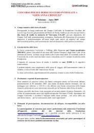
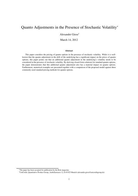
Jäckel [5]. Fur<strong>the</strong>rmore, <strong>the</strong> parametric form (11) is well supported by time series data. In Figure 1 <strong>the</strong> historical<br />
correlation between <strong>the</strong> VIX <strong>in</strong>dex and <strong>the</strong> US Dollar/Euro rate is plotted aga<strong>in</strong>st <strong>the</strong> product <strong>of</strong> <strong>the</strong> historical<br />
correlation between <strong>the</strong> S&P 500 <strong>in</strong>dex and <strong>the</strong> VIX <strong>in</strong>dex and <strong>the</strong> historical correlation between <strong>the</strong> S&P 500<br />
<strong>in</strong>dex and <strong>the</strong> US Dollar/Euro rate. The correlations for a specific day are calculated based on <strong>the</strong> returns <strong>of</strong> <strong>the</strong><br />
last 100 trad<strong>in</strong>g days. As visible <strong>in</strong> Figure 1 <strong>the</strong> realized correlation between <strong>the</strong> FX rate and <strong>the</strong> equity volatility<br />
is consistently positive s<strong>in</strong>ce November 2008 which has a volatility reduc<strong>in</strong>g effect under <strong>the</strong> quanto measure (see<br />
(4)). Fu<strong>the</strong>rmore, <strong>the</strong> realized correlation is most <strong>of</strong> <strong>the</strong> time very close to <strong>the</strong> correlation estimated us<strong>in</strong>g equation<br />
(11). Alternatively, one could also estimate <strong>the</strong> correlation ρν,F X directly based on historical data.<br />
After estimat<strong>in</strong>g <strong>the</strong> parameter ρν,F X, it rema<strong>in</strong>s to f<strong>in</strong>d <strong>the</strong> correlation ρS,F X by apply<strong>in</strong>g equation (6) and a root-<br />
Figure 1: Correlation between VIX <strong>in</strong>dex and US Dollar/Euro<br />
f<strong>in</strong>d<strong>in</strong>g algorithm to match <strong>the</strong> quanto forward given by <strong>the</strong> market. An application <strong>of</strong> <strong>the</strong> suggested calibration<br />
procedure to <strong>the</strong> S&P 500 <strong>in</strong>dex and <strong>the</strong> US Dollar/Euro rate for a maturity <strong>of</strong> T = 3 years and market data from<br />
May 27, 2011 yields <strong>the</strong> model parameters listed <strong>in</strong> Table 1.<br />
It is worth not<strong>in</strong>g that <strong>the</strong> choice <strong>of</strong> <strong>the</strong> correlation parameter ρν,F X has a significant impact on <strong>the</strong> model prices<br />
<strong>of</strong> quanto options as it determ<strong>in</strong>es <strong>the</strong> magnitude <strong>of</strong> <strong>the</strong> quanto adjustment <strong>in</strong> <strong>the</strong> volatility. Table 2 lists <strong>the</strong> price 5<br />
<strong>of</strong> a Euro quanto call option on <strong>the</strong> S&P 500 <strong>in</strong>dex with maturity <strong>of</strong> 3 years and strike equal to <strong>the</strong> spot <strong>of</strong> <strong>the</strong><br />
S&P 500 <strong>in</strong>dex for different values <strong>of</strong> <strong>the</strong> correlation parameter ρν,F X. For each choice <strong>of</strong> <strong>the</strong> parameter ρν,F X<br />
5 In this paper <strong>the</strong> prices <strong>of</strong> options are always expressed as a percentage <strong>of</strong> <strong>the</strong> underly<strong>in</strong>g spot as it is common <strong>in</strong> <strong>the</strong> OTC market.<br />
6<br />
(11)
Table 1: Model Parameters<br />
ν0 κ θ δ ρS,ν σF X ρS,F X ρν,F X<br />
0.175 0.103 0.131 0.187 -0.815 0.133 -0.63 0.51<br />
Table 2: Model prices for different correlation values<br />
ρν,F X 0.51 0.20 0.00<br />
<strong>Quanto</strong> Call Price 12.98 13.30 13.52<br />
<strong>the</strong> correlation ρS,F X is chosen such that <strong>the</strong> quanto forward is fitted <strong>in</strong> order to facilitate a proper comparison.<br />
The second row <strong>of</strong> Table 2 corresponds to <strong>the</strong> parametric form (11), however, o<strong>the</strong>r values for <strong>the</strong> correlation<br />
ρν,F X yield very different prices for <strong>the</strong> quanto call option although <strong>the</strong> price <strong>of</strong> <strong>the</strong> quanto forward rema<strong>in</strong>s <strong>the</strong><br />
same. We observe that <strong>the</strong> higher <strong>the</strong> correlation ρν,F X, <strong>the</strong> lower <strong>the</strong> quanto call option prices which can be well<br />
expla<strong>in</strong>ed by <strong>the</strong> fact that a higher correlation ρν,F X results <strong>in</strong> a lower long-term mean volatility ˆ θ under <strong>the</strong> quanto<br />
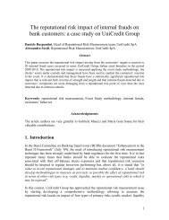
measure. Figure 2 plots <strong>the</strong> implied volatilities correspond<strong>in</strong>g to <strong>the</strong> 3 year quanto call options for different strikes<br />
and different volatility/FX correlation values. The graphs confirm that a change <strong>in</strong> <strong>the</strong> correlation ρν,F X results <strong>in</strong><br />
an almost parallel shift <strong>of</strong> <strong>the</strong> implied volatilities.<br />
In order to ga<strong>in</strong> an <strong>in</strong>tuition for <strong>the</strong>se observations we consider a Euro based trader who sold a Euro quanto option<br />
on <strong>the</strong> S&P 500 and is delta hedg<strong>in</strong>g <strong>the</strong> option position us<strong>in</strong>g a standard S&P 500 future and vega hedg<strong>in</strong>g us<strong>in</strong>g<br />
a standard variance swap or a VIX future. While all <strong>the</strong> hedge <strong>in</strong>struments are traded <strong>in</strong> US Dollar, <strong>the</strong> quanto<br />
option has no direct exposure to <strong>the</strong> US Dollar. Thus, <strong>the</strong> trader will need to setup a FX hedge <strong>in</strong> order to hedge<br />
<strong>the</strong> US Dollar exposure com<strong>in</strong>g from <strong>the</strong> hedge <strong>in</strong>struments. If <strong>the</strong> S&P 500 <strong>in</strong>dex or <strong>the</strong> volatility change, <strong>the</strong> US<br />
Dollar value <strong>of</strong> <strong>the</strong> hedge <strong>in</strong>struments changes which will cause <strong>the</strong> trader to dynamically rehedge <strong>the</strong> FX exposure<br />
depend<strong>in</strong>g on <strong>the</strong> movements <strong>of</strong> <strong>the</strong> underly<strong>in</strong>g and it’s volatility. Consequently, <strong>the</strong> equity/FX correlation ρS,F X<br />
toge<strong>the</strong>r with <strong>the</strong> equity volatility and <strong>the</strong> FX volatility <strong>in</strong>fluence <strong>the</strong> trader’s hedge due to <strong>the</strong> <strong>in</strong>teraction <strong>of</strong> <strong>the</strong><br />
delta hedge and <strong>the</strong> FX hedge. However, also <strong>the</strong> volatility/FX correlation ρν,F X toge<strong>the</strong>r with <strong>the</strong> volatility <strong>of</strong><br />
volatility and <strong>the</strong> FX volatility impact <strong>the</strong> hedge result <strong>in</strong> a similar way due to <strong>the</strong> <strong>in</strong>teraction <strong>of</strong> <strong>the</strong> vega hedge<br />
and <strong>the</strong> FX hedge. The first effect is well-known and taken <strong>in</strong>to account by <strong>the</strong> quanto adjustment <strong>in</strong> <strong>the</strong> drift <strong>of</strong><br />
<strong>the</strong> underly<strong>in</strong>g when pric<strong>in</strong>g quanto options <strong>in</strong> <strong>the</strong> standard framework. The second effect should not be ignored<br />
especially <strong>in</strong> <strong>the</strong> presence <strong>of</strong> a persistent positive volatility/FX correlation but it is only taken <strong>in</strong>to account by<br />
<strong>the</strong> additional quanto adjustment <strong>in</strong> <strong>the</strong> volatility - a term which is absent <strong>in</strong> <strong>the</strong> classical quanto option pric<strong>in</strong>g<br />
framework.<br />
5 Comparison with standard methods and <strong>the</strong> impact <strong>of</strong> <strong>the</strong> FX skew<br />
One <strong>in</strong>accuracy <strong>of</strong> our model is that it only assumes Black-Scholes dynamics for <strong>the</strong> FX rate and <strong>the</strong>reby ignores<br />
<strong>the</strong> implied volatility skew or smile which can be observed <strong>in</strong> currency option markets. Although this simplify<strong>in</strong>g<br />
assumption facilitated <strong>the</strong> derivation <strong>of</strong> closed-form solutions for quanto options, <strong>the</strong> question arises whe<strong>the</strong>r <strong>the</strong><br />
volatility skew on FX rate options has a significant impact on standard quanto options on <strong>the</strong> underly<strong>in</strong>g S and<br />
should be taken <strong>in</strong>to account when pric<strong>in</strong>g quanto options. In order to answer this question, we extend our model<br />
by <strong>in</strong>troduc<strong>in</strong>g a stochastic volatility also for <strong>the</strong> FX rate process. Consequently, <strong>the</strong> extended model is described<br />
by <strong>the</strong> equations (1), (2) and by <strong>the</strong> follow<strong>in</strong>g dynamics for Z Y/X under <strong>the</strong> foreign measure Q X :<br />
dZ Y/X (t) = (r X − r Y )Z Y/X (t)dt + νF X(t)Z Y/X (t)dW QX<br />
Z (t), ZY/X (0) = Z Y/X<br />
0<br />
dνF X(t) = κF X (θF X − νF X(t)) dt + δF XdW QX<br />
νF X (t), νF X(0) = νF X,0.<br />
7
Figure 2: Implied volatilities for different correlation values<br />
We denote <strong>the</strong> extended model as double SV model and note that <strong>the</strong> correlation matrix between <strong>the</strong> Brownian<br />
motions W QX QX<br />
S , Wν , W QX QX<br />
Z , Wν is given by<br />
⎛<br />
⎞<br />
1 ρS,ν ρS,Z ρS,νF X<br />
⎜ ρS,ν ⎜ 1 ρν,Z ρν,νF<br />
⎟<br />
X ⎟<br />
⎜ ρS,Z ρν,Z ⎜<br />
1 ρZ,νF<br />
⎟<br />
X ⎟<br />
⎝<br />
⎠ .<br />
ρS,νF X ρν,νF X ρZ,νF X 1<br />
We reduce <strong>the</strong> dimensionality <strong>of</strong> <strong>the</strong> correlation matrix by choos<strong>in</strong>g <strong>the</strong> parametric form:<br />
ρS,νF X = ρS,ZρZ,νF X , ρν,Z = ρS,νρS,Z, ρν,νF X = ρS,νρS,ZρZ,νF X ,<br />
which matches correlation assumptions made by Dimitr<strong>of</strong>f et al. [1] and also corresponds to <strong>the</strong> correlation<br />
parametrization with parameter β = 0 used by Jäckel [5]. 6 For <strong>the</strong> calibration <strong>of</strong> <strong>the</strong> double SV model we determ<strong>in</strong>e<br />
<strong>the</strong> stochastic volatility parameters <strong>of</strong> ν <strong>the</strong> same way we did before and <strong>in</strong> addition obta<strong>in</strong> <strong>the</strong> FX parameters<br />
νF X,0, κF X, θF X, δF X and ρZ,νF by an analog calibration to standard options on <strong>the</strong> FX rate. The correlation<br />
X<br />
parameter ρS,Z is <strong>the</strong>n set such that <strong>the</strong> model price <strong>of</strong> <strong>the</strong> quanto forward is match<strong>in</strong>g quanto forward given by <strong>the</strong><br />
market. In absence <strong>of</strong> closed-form solutions for <strong>the</strong> prices <strong>of</strong> <strong>the</strong> quanto forward and quanto options <strong>in</strong> <strong>the</strong> double<br />
SV model we apply standard Monte Carlo methods to compute <strong>the</strong>se prices numerically and use <strong>the</strong> follow<strong>in</strong>g<br />
equations <strong>in</strong> this context: 7,8<br />
F q (t, T ) = e (rY −r X )(T −t) E Q X<br />
C q (t, T, K) = e −rX (T −t) E Q X<br />
�<br />
S(T ) ZY/X (T )<br />
ZY/X �<br />
,<br />
(t)<br />
�<br />
(S(T ) − K) + Z Y/X (T )<br />
Z Y/X (t)<br />
6 Jäckel [5] demonstrated that <strong>the</strong> specific choice <strong>of</strong> <strong>the</strong> parameter β used <strong>in</strong> his correlation parametrization does not have a significant<br />
impact on <strong>the</strong> prices <strong>of</strong> quanto options as long as <strong>the</strong> model is always calibrated to a given quanto forward.<br />
7 See Jäckel [4] or Dimitr<strong>of</strong>f et al. [1] for a simple derivation <strong>of</strong> <strong>the</strong> equations.<br />
8 In <strong>the</strong> <strong>in</strong>terest <strong>of</strong> brevity, we do not perform <strong>the</strong> change <strong>of</strong> measure to <strong>the</strong> domestic risk-neutral measure Q Y for <strong>the</strong> double SV model<br />
which would results <strong>in</strong> similar additional quanto adjustments as seen <strong>in</strong> <strong>the</strong> previous sections.<br />
8<br />
�<br />
.
Table 3: Model Parameters for Double SV Model<br />
ν0 κ θ δ ρS,ν νF X,0 κF X θF X δF X ρZ,νF X ρS,Z<br />
0.175 0.103 0.131 0.187 -0.815 0.147 0.547 0.101 0.092 -0.34 0.62<br />
Table 4: Prices <strong>of</strong> quanto call options. The numbers <strong>in</strong> paren<strong>the</strong>ses are sample standard deviations.<br />
Strike Double SV model SV model DFAQ BS QFAQ BS QFAQ SV<br />
70 32.44 (0.013) 32.46 32.90 33.10 33.10<br />
80 25.21 (0.011) 25.24 25.75 26.03 26.03<br />
90 18.66 (0.010) 18.70 19.25 19.60 19.60<br />
100 12.95 (0.008) 12.98 13.54 13.94 13.94<br />
110 8.26 (0.007) 8.30 8.80 9.20 9.20<br />
120 4.80 (0.005) 4.82 5.22 5.56 5.56<br />
130 2.57 (0.004) 2.58 2.86 3.07 3.07<br />
Calibrat<strong>in</strong>g <strong>the</strong> double SV model to <strong>the</strong> same market data as used before, we obta<strong>in</strong> <strong>the</strong> model parameters listed <strong>in</strong><br />
Table 3.<br />
Based on <strong>the</strong> calibrated model parameters for <strong>the</strong> two stochastic volatility models we now compare <strong>the</strong> model<br />
prices for Euro quanto call options on <strong>the</strong> S&P 500 <strong>in</strong>dex with a maturity T = 3 years. We also <strong>in</strong>clude <strong>in</strong> our<br />
comparison option prices calculated us<strong>in</strong>g <strong>the</strong> follow<strong>in</strong>g three commonly used ad-hoc methods for quanto options:<br />
• Domestic-Forward-ATM-<strong>Quanto</strong> Black-Scholes (DFAQ BS) method<br />
• <strong>Quanto</strong>-Forward-ATM-<strong>Quanto</strong> Black-Scholes (QFAQ BS) method<br />
• <strong>Quanto</strong>-Forward-ATM-<strong>Quanto</strong> <strong>Stochastic</strong> <strong>Volatility</strong> (QFAQ SV) method<br />
The DFAQ BS method is simply us<strong>in</strong>g Black’s formula with <strong>the</strong> given quanto forward F q,market (T ), <strong>the</strong> discount<br />
factor belong<strong>in</strong>g to <strong>the</strong> payment currency Y and with a volatility for <strong>the</strong> underly<strong>in</strong>g equal to <strong>the</strong> implied volatility<br />
<strong>of</strong> <strong>the</strong> correspond<strong>in</strong>g non-quanto option with <strong>the</strong> same strike K and <strong>the</strong> same maturity T as <strong>the</strong> quanto option. 9<br />
The QFAQ BS method only differs from <strong>the</strong> DFAQ BS method by us<strong>in</strong>g a quanto forward adjusted volatility for<br />
<strong>the</strong> underly<strong>in</strong>g which is <strong>the</strong> implied volatility <strong>of</strong> <strong>the</strong> non-quanto option with <strong>the</strong> same maturity T but with <strong>the</strong><br />
adjusted strike ˆ K = K × F X (T )/F q,market (T ) where F X (T ) is <strong>the</strong> forward <strong>of</strong> <strong>the</strong> underly<strong>in</strong>g asset under <strong>the</strong><br />
foreign measure Q X . 10 F<strong>in</strong>ally, <strong>the</strong> QFAQ SV method is us<strong>in</strong>g <strong>the</strong> closed-form solution for non-quanto standard<br />
options <strong>in</strong> <strong>the</strong> assumed stochastic volatility model for <strong>the</strong> underly<strong>in</strong>g S but replac<strong>in</strong>g <strong>the</strong> forward with <strong>the</strong> quanto<br />
forward F q,market (T ) and <strong>the</strong> discount factor with <strong>the</strong> discount factor belong<strong>in</strong>g to <strong>the</strong> payment currency Y . All<br />
three approximations are commonly used <strong>in</strong> practice as outl<strong>in</strong>ed by Jäckel [5] from which we have also borrowed<br />
<strong>the</strong> notation for <strong>the</strong> three methods. Please note that all three common methods do not feature <strong>the</strong> additional quanto<br />
adjustment <strong>in</strong> <strong>the</strong> volatility.<br />
The results are summarized <strong>in</strong> Table 4 and reveal that <strong>the</strong> three standard methods produce prices which are almost<br />
100 basis po<strong>in</strong>ts higher than <strong>the</strong> prices <strong>of</strong> our two stochastic volatility models. 11,12 These higher prices can be<br />
expla<strong>in</strong>ed by <strong>the</strong> lack <strong>of</strong> <strong>the</strong> quanto adjustment <strong>in</strong> <strong>the</strong> volatility which causes <strong>the</strong> standard methods to use a higher<br />
effective volatility for <strong>the</strong> pric<strong>in</strong>g <strong>of</strong> quanto options. Note that <strong>the</strong> observed price differences are above <strong>the</strong> usual<br />
bid/<strong>of</strong>fer spreads <strong>of</strong> less 50 basis po<strong>in</strong>ts for quanto options <strong>in</strong> <strong>the</strong> OTC market which strongly suggests that ignor<strong>in</strong>g<br />
<strong>the</strong> quanto adjustment <strong>in</strong> <strong>the</strong> volatility can lead to mispric<strong>in</strong>g <strong>of</strong> quanto options. In contrast to this, <strong>the</strong> prices <strong>of</strong><br />
our reduced stochastic volatility model <strong>of</strong> Section 2 agree well with prices <strong>of</strong> <strong>the</strong> fully fledged double SV model<br />
listed <strong>in</strong> Table 4. This <strong>in</strong>dicates that <strong>the</strong> price impact <strong>of</strong> <strong>the</strong> FX implied volatility skew on standard quanto options<br />
is small and that our closed-form solutions derived <strong>in</strong> Section 3 could well be used for an efficient pric<strong>in</strong>g and risk<br />
9 In order to rule out that calibration errors result<strong>in</strong>g from <strong>the</strong> calibration <strong>of</strong> <strong>the</strong> stochastic volatility model to <strong>the</strong> market data potentially<br />
overshadow <strong>the</strong> model comparison we use <strong>the</strong> implied volatilities <strong>in</strong>duced by <strong>the</strong> stochastic volatility parameter listed <strong>in</strong> Table 1 throughout <strong>the</strong><br />
comparison.<br />
10 Intuitively speak<strong>in</strong>g, <strong>the</strong> QFAQ BS method is try<strong>in</strong>g to reflect <strong>the</strong> different ”moneyness” <strong>of</strong> <strong>the</strong> quanto option <strong>in</strong> comparison to <strong>the</strong> nonquanto<br />
option with <strong>the</strong> same strike caused by <strong>the</strong> different forwards.<br />
11 The prices <strong>of</strong> options as well as <strong>the</strong> strikes are expressed as a percentage <strong>of</strong> <strong>the</strong> underly<strong>in</strong>g spot <strong>in</strong> <strong>the</strong> Table 4.<br />
12 Note that <strong>the</strong> QFAQ BS method and <strong>the</strong> QFAQ SV method yield exactly <strong>the</strong> same prices <strong>in</strong> our model sett<strong>in</strong>g which is due to <strong>the</strong> fact that<br />
<strong>the</strong> price functions for a non-quanto call option <strong>in</strong> <strong>the</strong> Black Scholes model and <strong>the</strong> stochastic volatility model are both homogeneous with<br />
respect to <strong>the</strong> forward and <strong>the</strong> strike.<br />
9
management <strong>of</strong> standard quanto options without a material loss <strong>of</strong> exactness even though only at-<strong>the</strong>-money FX<br />
implied volatilities are used.<br />
6 Conclusion<br />
We have <strong>in</strong>troduced a model for <strong>the</strong> pric<strong>in</strong>g <strong>of</strong> quanto options which features stochastic volatility for <strong>the</strong> underly<strong>in</strong>g.<br />
Closed-form pric<strong>in</strong>g formulas for <strong>the</strong> quanto forward and standard quanto options have been derived for <strong>the</strong><br />
model which facilitate a fast calibration <strong>of</strong> <strong>the</strong> model and an efficient pric<strong>in</strong>g and risk management <strong>of</strong> standard<br />
quanto options without <strong>the</strong> need <strong>of</strong> us<strong>in</strong>g Monte Carlo methods or numerical solutions <strong>of</strong> PDEs. We found that <strong>in</strong><br />
addition to <strong>the</strong> common quanto adjustment <strong>in</strong> <strong>the</strong> drift <strong>of</strong> <strong>the</strong> underly<strong>in</strong>g a quanto adjustment <strong>in</strong> <strong>the</strong> volatility needs<br />
to be considered. The impact <strong>of</strong> this additional quanto adjustment has been studied and shown to be <strong>of</strong> significance<br />
for <strong>the</strong> prices <strong>of</strong> standard quanto options. Fur<strong>the</strong>rmore, we have numerically studied <strong>the</strong> accuracy <strong>of</strong> <strong>the</strong> obta<strong>in</strong>ed<br />
quanto option prices <strong>in</strong> <strong>the</strong> framework <strong>of</strong> a double stochastic volatility model with stochastic volatility for both <strong>the</strong><br />
underly<strong>in</strong>g and <strong>the</strong> FX process. In this study, we have observed that our stochastic volatility model only produced<br />
very small price differences <strong>in</strong> comparison to <strong>the</strong> benchmark prices <strong>of</strong> <strong>the</strong> double stochastic volatility model and<br />
has <strong>the</strong> advantage <strong>of</strong> <strong>of</strong>fer<strong>in</strong>g closed-form solutions. In addition, three commonly used methods for <strong>the</strong> pric<strong>in</strong>g <strong>of</strong><br />
quanto options have been <strong>in</strong>cluded <strong>in</strong> <strong>the</strong> numerical study with <strong>the</strong> observation that <strong>the</strong> standard methods produce<br />
price differences <strong>in</strong> comparison to <strong>the</strong> two stochastic volatility models which are above <strong>the</strong> usual bid/<strong>of</strong>fer spreads<br />
and are due to <strong>the</strong> miss<strong>in</strong>g quanto adjustment <strong>in</strong> <strong>the</strong> volatility.<br />
It is clear that <strong>the</strong> volatility chang<strong>in</strong>g effect <strong>of</strong> <strong>the</strong> additional quanto adjustment does not only have an impact on<br />
standard quanto options but also on exotic quanto options with high vega exposure like barrier options for <strong>in</strong>stance.<br />
In <strong>the</strong> <strong>in</strong>terest <strong>of</strong> brevity, we defer <strong>the</strong> analysis <strong>of</strong> exotic quanto options as well as a more extensive analysis <strong>of</strong> <strong>the</strong><br />
impact <strong>of</strong> <strong>the</strong> FX smile or skew on quanto options to future work.<br />
Alexander Giese is head <strong>of</strong> <strong>the</strong> equity and commodity quant team at UniCredit. He would like to thank Dong Qu, Thomas<br />
Goll, Jan Maruhn, Lionel Viet, Francesco Robertella and two anonymous referees for helpful comments and suggestions.<br />
Email: alexander.giese@unicreditgroup.de<br />
References<br />
[1] G. Dimitr<strong>of</strong>f, A. Szimayer, and A. Wagner. <strong>Quanto</strong> option pric<strong>in</strong>g <strong>in</strong> <strong>the</strong> parsimonious heston model. Berichte des Fraunh<strong>of</strong>er<br />
ITWM, (174), 2009.<br />
[2] F. Gerlich, A. Giese, J.H. Maruhn, and E.W. Sachs. Parameter identification <strong>in</strong> f<strong>in</strong>ancial market models with a feasible<br />
po<strong>in</strong>t sqp algorithm. Journal <strong>of</strong> Computational Optimization and Applications, 2010.<br />
[3] S. L. Heston. A closed-form solution for options with stochastic volatility with applications to bond and currency options.<br />
The Review <strong>of</strong> F<strong>in</strong>ancial Studies, 6(2):327343, 1993.<br />
[4] P. Jäckel. <strong>Quanto</strong> skew. www.jaeckel.org/<strong>Quanto</strong>Skew.pdf, 2009.<br />
[5] P. Jäckel. <strong>Quanto</strong> skew with stochastic volatility. www.jaeckel.org/<strong>Quanto</strong>SkewWith<strong>Stochastic</strong><strong>Volatility</strong>.pdf, 2010.<br />
[6] A. Lipton and A. Sepp. <strong>Stochastic</strong> volatility models and kelv<strong>in</strong> waves. Journal <strong>of</strong> Physics A: Ma<strong>the</strong>matical and Theoretical,<br />
41(32), 2008.<br />
[7] R. Lord and C. Kahl. Optimal fourier <strong>in</strong>version <strong>in</strong> semi-analytical option pric<strong>in</strong>g. Journal <strong>of</strong> Computational F<strong>in</strong>ance,<br />
10(4):1–30, 2007.<br />
[8] E. Re<strong>in</strong>er. <strong>Quanto</strong> mechanics. Risk, 5(3):59–63, 1992.<br />
[9] R. Schöbel and J. Zhu. <strong>Stochastic</strong> volatility with an ornste<strong>in</strong>-uhlenbeck process: an extension. European F<strong>in</strong>ance Review,<br />
4:23–46, 1999.<br />
10
A Appendix<br />
Lemma 1. Let ν be a mean-reversion Ornste<strong>in</strong>-Uhlenbeck process under <strong>the</strong> measure Q, i.e.:<br />
Fu<strong>the</strong>rmore, let <strong>the</strong> function y be def<strong>in</strong>ed as<br />
dν(t) = κ (θ − ν(t)) dt + δdW Q (t), ν(0) = ν0.<br />
�<br />
Q<br />
y (t, T, ν(t)) = E e −s1<br />
� Tt<br />
ν(u) 2 � Tt<br />
du−s2 ν(u)du+s3v(T ) �<br />
for arbitrary complex numbers s1,s2, s3 and −s1ν(u) 2 − s2ν(u) is lower bounded. Then y has <strong>the</strong> follow<strong>in</strong>g solution:<br />
where <strong>the</strong> function D is given by<br />
with<br />
y (t, T, ν(t)) = D (t, T, ν(t), s1, s2, s3)<br />
D (t, T, ν(t), s1, s2, s3) = e 1 2 A(t,T,s1,s2)ν(t) 2 +B(t,T,s1,s2,s3)ν(t)+C(t,T,s1,s2,s3)<br />
A (t, T, s1, s2) = κ γ1<br />
−<br />
δ2 δ2 Ψ (γ1, γ2)<br />
Φ (γ1, γ2)<br />
B (t, T, s1, s2, s3) =<br />
κθγ1 − γ2γ3 + γ3Ψ (γ1, γ2)<br />
δ 2 γ1Φ (γ1, γ2)<br />
− κθ<br />
δ 2<br />
C (t, T, s1, s2, s3) = − 1<br />
κ<br />
ln (Φ (γ1, γ2)) + (T − t)<br />
�<br />
2 2<br />
2 2 2<br />
κ θ γ1 − γ<br />
+<br />
2� 3<br />
2δ2γ 3 � �<br />
s<strong>in</strong>h (γ1 (T − t))<br />
− γ1 (T − t)<br />
1 Φ (γ1, γ2)<br />
� �<br />
cosh (γ1 (T − t)) − 1<br />
Φ (γ1, γ2)<br />
Pro<strong>of</strong>. See <strong>the</strong> appendix <strong>of</strong> Schöbel and Zhu [9].<br />
+ (κθγ1 − γ2γ3) γ3<br />
δ2γ 3 1<br />
Ψ (γ1, γ2) = s<strong>in</strong>h (γ1 (T − t)) + γ2 cosh (γ1 (T − t))<br />
Φ (γ1, γ2) = cosh (γ1 (T − t)) + γ2 s<strong>in</strong>h (γ1 (T − t))<br />
γ1 = � 2δ2s1+κ2 γ2 = 1 � 2 �<br />
κ − 2δ s3<br />
γ1<br />
γ3 = κ 2 θ − s2δ 2 .<br />
11