Consistent Pricing of CMS and CMS Spread Options - UniCredit ...
Consistent Pricing of CMS and CMS Spread Options - UniCredit ...
Consistent Pricing of CMS and CMS Spread Options - UniCredit ...

You also want an ePaper? Increase the reach of your titles
YUMPU automatically turns print PDFs into web optimized ePapers that Google loves.
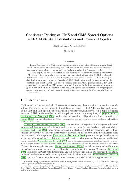
<strong>Consistent</strong> <strong>Pricing</strong> <strong>of</strong> <strong>CMS</strong> <strong>and</strong> <strong>CMS</strong> <strong>Spread</strong> <strong>Options</strong><br />
with SABR-like Distributions <strong>and</strong> Power-t Copulas<br />
Andreas K.H. Geisselmeyer ∗<br />
March, 2012<br />
Abstract<br />
Today, European-style <strong>CMS</strong> spread options are <strong>of</strong>ten priced with a bivariate normal distribution,<br />
which arises when modelling the <strong>CMS</strong> rates with two correlated Gaussian stochastic<br />
processes, or, equivalently, two normal marginals coupled with a Gaussian copula.<br />
In this paper, we relax the rather ad-hoc assumption <strong>of</strong> bivariate normally distributed<br />
<strong>CMS</strong> rates. First, we replace the normal marginal distributions with SABR-like skewed-t<br />
distributions. By means <strong>of</strong> a Power-t copula, we then derive a skewed <strong>and</strong> fat-tailed joint<br />
distribution as a good proxy to a bivariate SABR distribution, which is nonetheless simple,<br />
tractable <strong>and</strong> well-behaved. We present efficient semi-analytical pricing formulas for <strong>CMS</strong><br />
spread options (as well as <strong>CMS</strong> swaps, caps <strong>and</strong> floors as the limiting cases) <strong>and</strong> achieve a<br />
good match <strong>of</strong> the SABR swaption, <strong>CMS</strong> <strong>and</strong> <strong>CMS</strong> spread option market. For larger spread<br />
option maturities, we find indications for possible inconsistencies in the <strong>CMS</strong> <strong>and</strong> <strong>CMS</strong> spread<br />
option market.<br />
1 Introduction<br />
<strong>CMS</strong> spread options are typically European-style today <strong>and</strong> therefore <strong>of</strong> a comparatively simple<br />
nature. The problem <strong>of</strong> their consistent modelling, ie. recovering the SABR swaption smile as well<br />
as the <strong>CMS</strong> <strong>and</strong> <strong>CMS</strong> spread option market in a realistic way, is, however, still a topic <strong>of</strong> ongoing<br />
research. SABR is the st<strong>and</strong>ard model for pricing interest rate swaptions, cf. Hagan, Kumar,<br />
Lesniewski, <strong>and</strong> Woodward [2002], <strong>and</strong> is also the basis for <strong>CMS</strong> pricing via <strong>CMS</strong> replication, cf.<br />
Hagan [2003]. In the following, we briefly summarise the work on European-style spread options<br />
<strong>of</strong> the past decade.<br />
Cherubini, Luciano, <strong>and</strong> Vecchiato [2001] use Archimedean copulas with marginals calibrated<br />
to historical data to give price bounds <strong>and</strong> pricing formulas for multivariate contingent claims.<br />
Dempster <strong>and</strong> Hong [2001] price spread options in a stochastic volatility framework via FFT assuming<br />
the existence <strong>of</strong> the joint characteristic function, eg. in the case when the underliers share<br />
the stochastic variance process. Carmona <strong>and</strong> Durrleman [2003] present a comprehensive survey<br />
on the available models <strong>and</strong> tools for spread option pricing with a special focus on commodity <strong>and</strong><br />
energy markets. Alex<strong>and</strong>er <strong>and</strong> Scourse [2003] use a bivariate lognormal mixture model to introduce<br />
a slight skew <strong>and</strong> semi-heavy tails in the joint distribution <strong>and</strong> to account for the correlation<br />
“frown”, ie. the correlation skew. Bennett <strong>and</strong> Kennedy [2004] model the marginals with a mixture<br />
<strong>of</strong> lognormals <strong>and</strong> use a perturbed Gaussian copula for pricing quanto FX options. Berrahoui<br />
[2004] calculates the <strong>CMS</strong> rate distributions via call spreads thus taking into account the volatility<br />
smile <strong>and</strong> further applies a Gaussian copula calibrated to historical data. Benhamou <strong>and</strong> Croissant<br />
[2007] apply a Gaussian copula to marginals obtained via SABR local time approximations.<br />
∗ Unicredit Group, Quantitative Product Group, Rates Quants, Arabellastrasse 12, D-81925 Munich, Germany,<br />
<strong>and</strong>reas.geisselmeyer@unicreditgroup.de.<br />
I would like to thank Dongning Qu for suggesting this project <strong>and</strong> many helpful comments. I would also like to<br />
thank Robert Br<strong>and</strong>, Stephane Capet, Daniel Dreher, Ricardo Rueda-Nagel <strong>and</strong> Rol<strong>and</strong>o Santambrogio for many<br />
insightful discussions.<br />
1
Shaw <strong>and</strong> Lee [2007] <strong>and</strong> the references therein tackle Student-t copulas based on general multivariate<br />
t distributions.<br />
With the financial crisis, spread option modelling more or less went back to the bivariate<br />
normal case, while fixing some details. Recently though, copulas have attracted attention again.<br />
Liebscher [2008] introduces multivariate product copulas, which in particular allow to create<br />
new asymmetric copulas out <strong>of</strong> existing copulas. Based on these results, Andersen <strong>and</strong> Piterbarg<br />
[2010] present Power copulas <strong>and</strong> apply a Power-Gaussian copula to <strong>CMS</strong> spread option pricing,<br />
thus generating a skew in the joint distribution. Similarly, Austing [2011] <strong>and</strong> Elices <strong>and</strong> Fouque<br />
[2012] give constructions <strong>of</strong> skewed joint distributions, the former in the FX context via best-<strong>of</strong><br />
options, the latter via a perturbed Gaussian copula derived with asymptotic expansion techniques<br />
from the transition probabilities <strong>of</strong> a stochastic volatility model. Piterbarg [2011] derives necessary<br />
<strong>and</strong> sufficient conditions for the existence <strong>of</strong> a joint distribution consistent with vanilla <strong>and</strong> exotic<br />
prices in a <strong>CMS</strong> spread, FX cross-rate or equity basket option context. McCloud [2011] shows<br />
the dislocation <strong>of</strong> the <strong>CMS</strong> <strong>and</strong> <strong>CMS</strong> spread option market in the recent past <strong>and</strong> detects it<br />
with bounds from a copula based approach. Kienitz [2011] presents an extrapolation method<br />
for numerically obtained SABR probability distributions <strong>and</strong> applies Markovian projection to a<br />
bivariate SABR model.<br />
To date, to the best <strong>of</strong> our knowledge, there is no model in the spread option literature that<br />
takes into account the important features <strong>of</strong> a bivariate SABR distribution, ie. skew <strong>and</strong> fat<br />
tails in the joint probability distribution. Often, light-tailed distributions such as the bivariate<br />
normal, or semi-heavy-tailed <strong>and</strong> slightly skewed distributions such as lognormal mixtures are<br />
in use. Numerically-obtained SABR marginal distributions are not very tractable (issues with<br />
efficiency/accuracy/interpolation/extrapolation) <strong>and</strong> usually coupled with simple copulas such as<br />
the Gaussian copula which leads to unnatural joint distributions.<br />
The aim <strong>of</strong> this paper is to construct a <strong>CMS</strong> rate joint distribution with fat tails <strong>and</strong> skew which<br />
is close to a bivariate SABR distribution, but still manageable <strong>and</strong> well-behaved. We achieve this<br />
with a copula approach. We use the SABR-like skewed-t distribution to get a grip at the SABR<br />
probability distribution. Such distributions are simple, tractable <strong>and</strong> well-behaved, <strong>and</strong> can take<br />
into account skew <strong>and</strong> fat tails <strong>of</strong> the SABR distribution. We then apply a Power-t copula which is<br />
rich enough to generate a natural joint distribution with skew <strong>and</strong> heavy tails, but simple enough<br />
to maintain tractability. From there, we present semi-analytical pricing formulas for <strong>CMS</strong> spread<br />
options (<strong>and</strong> <strong>CMS</strong> swaps, caps <strong>and</strong> floors as the limiting cases) <strong>and</strong> are able to achieve a good<br />
fit to the swaption, <strong>CMS</strong> <strong>and</strong> <strong>CMS</strong> spread option market. For larger maturities <strong>and</strong> high strikes,<br />
skewed-t marginals lead to consistently higher <strong>CMS</strong> spread cap prices than the market (due to<br />
more probability mass in the tails), which is an indication for possible inconsistencies in the <strong>CMS</strong><br />
<strong>and</strong> <strong>CMS</strong> spread option market.<br />
The rest <strong>of</strong> the paper is organised as follows. In Section 2, we review st<strong>and</strong>ard European-style<br />
<strong>CMS</strong> spread options, introduce our notation <strong>and</strong> outline the main pricing problem. In Section<br />
3, we present the different marginal distributions we will use, from normal marginals to SABR<br />
marginals <strong>and</strong> SABR-like skewed-t marginals. We apply skewed-t distributions for the first time<br />
in the spread option literature. In Section 4, we recall some known <strong>and</strong> less-known results on<br />
copulas <strong>and</strong> review Gaussian, Power-Gaussian <strong>and</strong> t copulas. We then present the Power-t copula<br />
as a special case <strong>of</strong> Power copulas, which has not been used in the spread option literature before.<br />
Section 5 presents the pricing formulas for <strong>CMS</strong> caps <strong>and</strong> <strong>CMS</strong> spread caps (with <strong>CMS</strong> floors,<br />
<strong>CMS</strong> spread floors <strong>and</strong> <strong>CMS</strong> swaps following immediately). Section 6 gives numerical results. We<br />
show calibrations for the Gaussian copula with normal marginals (the st<strong>and</strong>ard bivariate normal<br />
model), the Power-Gaussian copula with normal marginals <strong>and</strong> the Power-t copula with skewed-t<br />
marginals. We further analyse how the different choices <strong>of</strong> marginals <strong>and</strong> copulas affect the prices<br />
<strong>of</strong> <strong>CMS</strong> caps, <strong>CMS</strong> spread digitals <strong>and</strong> <strong>CMS</strong> spread options. Section 7 concludes.<br />
2
2 The <strong>Pricing</strong> Problem<br />
Let S1 <strong>and</strong> S2 be two <strong>CMS</strong> rates with different tenors, eg. 10y <strong>and</strong> 2y, <strong>and</strong> 0 = T0 < T1 < · · · <<br />
Tn+1 a set <strong>of</strong> equally-spaced dates. St<strong>and</strong>ard <strong>CMS</strong> spread options are either caps or floors <strong>and</strong><br />
thus a sum <strong>of</strong> <strong>CMS</strong> spread caplets/floorlets with pay<strong>of</strong>fs<br />
h(S1(Ti), S2(Ti)) = τi max(ω(S1(Ti) − S2(Ti) − K), 0), i = 1, . . . , n<br />
where ω = ±1 <strong>and</strong> K a fixed strike. S1 <strong>and</strong> S2 are fixed at Ti, payment <strong>of</strong> h(S1(Ti), S2(Ti)) usually<br />
occurs at Ti+1, τi = Ti+1 − Ti is a year fraction, i = 1, . . . , n.<br />
The present value <strong>of</strong> a <strong>CMS</strong> spread cap/floor with maturity Tn+1 is<br />
n<br />
τiP (0, Ti+1) Ti+1 [max(ω(S1(Ti) − S2(Ti) − K), 0)] .<br />
i=1<br />
Expectations are taken under the Ti+1-forward measures. In the Euro area, fixing/payment dates<br />
are typically 3m-spaced. Note that the first caplet/floorlet which is fixed at T0 is excluded. When<br />
S2 is removed from the pay<strong>of</strong>f, we arrive at a <strong>CMS</strong> cap/floor, when we replace S2 with a 3m-<br />
Euribor, we obtain a <strong>CMS</strong> swap. Our pricing problem is therefore <strong>of</strong> the form<br />
V = Tp [max(ω(S1(T ) − S2(T ) − K), 0)]<br />
∞ ∞<br />
= h(s1, s2)ψ(s1, s2)ds1ds2<br />
−∞<br />
−∞<br />
with Tp ≥ T <strong>and</strong> ψ(s1, s2) the joint probability density <strong>of</strong> S1(T ) <strong>and</strong> S2(T ).<br />
In the following, we will work on a filtered probability space (Ω, , F, ), where = {Ft}t≥0<br />
denotes a filtration <strong>of</strong> F satisfying the usual conditions. We assume the existence <strong>of</strong> equivalent<br />
martingale measures <strong>and</strong> write [·] for the expected value w.r.t. such measures. We assume<br />
that the pay<strong>of</strong>f h(S1(T ), S2(T )) is FT -measurable <strong>and</strong> satisfies the necessary integrability<br />
conditions.<br />
For a bivariate normal distribution, the joint density function is available in closed form.<br />
Otherwise, this is rarely the case. We can, however, always represent a joint density in terms<br />
<strong>of</strong> its marginals <strong>and</strong> a (unique) copula (Sklar’s theorem). Let Ψ(s1, s2) be the joint cumulative<br />
distribution function (cdf), Ψi(si), i = 1, 2, the marginal cdfs, ψi(si), i = 1, 2, the marginal<br />
densities <strong>and</strong> C(u1, u2) a copula. Then<br />
Ψ(s1, s2) = C Ψ1(s1), Ψ2(s2) <br />
ψ(s1, s2) = ∂2<br />
C<br />
∂u1∂u2<br />
Ψ1(s1), Ψ2(s2) ψ1(s1)ψ2(s2)<br />
<strong>and</strong> it follows that<br />
∞ ∞<br />
∂<br />
V = h(s1, s2)<br />
2<br />
C<br />
∂u1∂u2<br />
Ψ1(s1), Ψ2(s2) ψ1(s1)ψ2(s2)ds1ds2.<br />
−∞<br />
−∞<br />
If we can represent the above 2d integral as a 1d integral, pricing becomes efficient.<br />
3 Marginal Distributions<br />
In this section, we present the different marginal distributions which we will use, from normal<br />
marginals to SABR marginals <strong>and</strong> SABR-like skewed-t marginals. Normal marginals will be<br />
used together with a Gaussian copula (the st<strong>and</strong>ard model), but also in the Power-Gaussian<br />
copula extension. We present the main properties (<strong>and</strong> peculiarities) <strong>of</strong> the (numerical) SABR<br />
distribution <strong>and</strong> finally the SABR-like skewed-t distribution, which will be applied in a Power-t<br />
copula setting.<br />
3
3.1 Gaussian Marginals<br />
We assume that the <strong>CMS</strong> rates S1 <strong>and</strong> S2 follow Gaussian processes:<br />
dSi(t) = σidW Tp<br />
i , Si(0) = Tp [Si(T )], i = 1, 2<br />
W Tp denotes a st<strong>and</strong>ard Wiener process w.r.t. the Tp-forward measure. The volatilities σi are<br />
chosen constant. Naturally, <strong>CMS</strong> rates are martingales under their respective annuity measure.<br />
We can assume no drifts under the Tp-forward measure by using the convexity-adjust <strong>CMS</strong> rate<br />
Si(0) = Tp [Si(T )] with T the fixing date.<br />
3.2 SABR Marginals<br />
We assume that the <strong>CMS</strong> rates S1 <strong>and</strong> S2 follow SABR processes:<br />
dSi(t) = αi(t)Si(t) βi Ai(T )<br />
dWi , Si(0) = Si,0<br />
Ai(T )<br />
dαi(t) = νiαi(t)dZi ,<br />
d〈Wi, Zi〉(t) = ρidt<br />
αi(0) = αi, i = 1, 2<br />
Ai(T )<br />
αi determines the swaption volatility level, βi <strong>and</strong> ρi the skew <strong>and</strong> νi the volatility smile. W<br />
<strong>and</strong> ZAi(T ) denote st<strong>and</strong>ard Wiener processes w.r.t. the Ai(T )-annuity measure. To obtain<br />
marginal SABR densities ψ Tp<br />
i<br />
(·) <strong>and</strong> cdfs ΨTp<br />
i (·) under the Tp-forward measure, we either use<br />
<strong>CMS</strong> digitals (caplet spreads) obtained via <strong>CMS</strong> replication, cf. Hagan [2003]<br />
Ψ Tp<br />
i (x) = 1 + ∂ETp (max(Si(T ) − x, 0))<br />
∂x<br />
ψ Tp<br />
i (x) = ∂2E Tp (max(Si(T ) − x, 0))<br />
∂x2 or apply the above formulas to payer swaption spreads to obtain ψ<br />
Andersen <strong>and</strong> Piterbarg [2010], Section 16.6.9:<br />
Ψ Tp<br />
i (x) =<br />
x<br />
−∞<br />
Gi(u, Tp)<br />
Gi(Si,0, Tp)<br />
ψ Tp<br />
i (x) = Gi(x, Tp)<br />
Gi(Si,0, Tp)<br />
)<br />
ψAi(T i (u)du<br />
)<br />
ψAi(T i (x).<br />
Ai(T )<br />
i<br />
(·) <strong>and</strong> then relate, cf.<br />
G arises from the change <strong>of</strong> measure from the Ai(T )-annuity measure to the Tp-forward measure<br />
P (·,Tp)<br />
<strong>and</strong> approximates the quotient Ai(·) via a yield curve model, cf. Hagan [2003], We find that<br />
both approaches produce nearly identical Tp-forward measure densities <strong>and</strong> cdfs. This implies<br />
that when we are able to recover <strong>CMS</strong> caplet prices (from <strong>CMS</strong> replication) with a density ψ∗ , we<br />
also recover SABR swaption prices with the density transform from above (<strong>and</strong> vice versa).<br />
Although it is desirable to use SABR marginals for spread option pricing, there are a few issues<br />
that complicate matters, cf. Andersen <strong>and</strong> Piterbarg [2005], Henry-Labordre [2008], Jourdain<br />
[2004]:<br />
• β = 1: For ρ > 0, S is not a martingale (explosion).<br />
• β ∈ (0, 1): S = 0 is an attainable boundary that either is absorbing ( 1 ≤ β < 1) or has to<br />
be chosen absorbing (0 < β < 1<br />
2 ) to avoid arbitrage1 .<br />
• β = 0: S can become negative.<br />
Usually, the SABR model behaves fairly well around at-the-money. We now have a brief look<br />
at what happens far-from-the-money (low strikes <strong>and</strong> high strikes).<br />
1 The arbitrage opportunity that arises when choosing a reflecting boundary is quite theoretical. S is, however,<br />
not a martingale anymore.<br />
4<br />
2
Low Strikes:<br />
• β = 1: This case is not really relevant for interest rate modelling unless ν is set to 0<br />
(lognormal model).<br />
• β ∈ (0, 1): This case is typical for the Euro markets. For low forwards <strong>and</strong> high volatilities,<br />
the probability <strong>of</strong> absorption can be quite high which in terms <strong>of</strong> financial modelling is<br />
unpleasant.<br />
The SABR density is not available in (semi-)analytical form. The st<strong>and</strong>ard volatility formula<br />
from Hagan, Kumar, Lesniewski, <strong>and</strong> Woodward [2002] applied to payer swaption spreads<br />
leads to negative probabilities when ν 2 T ≪ 1 does not hold (the singular perturbation<br />
techniques fail), the density formula from Hagan, Lesniewski, <strong>and</strong> Woodward [2005] behaves<br />
better but also gets less accurate the higher ν 2 T is (the asymptotic expansions fail) <strong>and</strong><br />
Monte Carlo is converging too slowly.<br />
• β = 0: This can be an interesting alternative in low interest rate environments. The density<br />
is purely diffusive.<br />
High Strikes: Generally, it is problematic to apply a model far away from the strike region it<br />
has been calibrated to. In case <strong>of</strong> the SABR model, the missing mean-reverting drift also leads to<br />
too high volatilities in the right wing.<br />
3.3 Skewed-t Marginals<br />
Due to the many issues we face in the relevant case β ∈ (0, 1), we will not use numerically<br />
computed SABR distributions directly. We instead resort to mapping the important features<br />
<strong>of</strong> the SABR distribution (location, scale, skew <strong>and</strong> kurtosis/tail behaviour) to a well-behaved<br />
<strong>and</strong> tractable distribution: the skewed-t distribution. This way, we also solve the problem <strong>of</strong><br />
interpolation/extrapolation. As long as the numerical SABR distribution is not too distorted<br />
(ν 2 T ≪ 1), we will achieve a surprisingly good fit. When the SABR volatility formula starts to<br />
induce negative probabilities, the fitting quality will <strong>of</strong> course deteriorate. Skewed-t distributions<br />
have not been used in the spread option literature before.<br />
We derive the skewed-t distribution in steps starting with the Student-t distribution. The<br />
Student-t distribution with d degrees <strong>of</strong> freedom has the density<br />
fd(x) =<br />
d+1 Γ( 2 )<br />
Γ( d<br />
2 )√ <br />
1 +<br />
dπ<br />
x2<br />
−<br />
d<br />
d+1<br />
2<br />
where Γ denotes the Gamma function. Introducing location <strong>and</strong> scale parameters µ <strong>and</strong> σ, we get<br />
fµ,σ,d(x) = 1<br />
σ fd<br />
<br />
x − µ<br />
.<br />
σ<br />
Introducing a skew parameter ε, cf. Fern<strong>and</strong>ez <strong>and</strong> Steel [1996], leads to<br />
<br />
<br />
x<br />
<br />
fd (εx) 1lx
Fd <strong>and</strong> F −1<br />
d denote cdf <strong>and</strong> inverse cdf <strong>of</strong> the Student-t distribution. With ε = 1 <strong>and</strong> d = ∞, we<br />
recover the normal distribution with mean µ <strong>and</strong> st<strong>and</strong>ard deviation σ. With µ = 0, σ = 1 <strong>and</strong><br />
ε = 1, we recover the Student-t distribution.<br />
ε < 1 produces a negative skew, ε > 1 a positive skew, cf. Figure 1. We see that with a<br />
negative/positive skew, the expected value is left/right <strong>of</strong> the peak respectively. Note that the<br />
expected value does not coincide with parameter µ when ε = 1.<br />
Figure 1: Skewed-t densities with left skew (red) <strong>and</strong> right skew (blue) <strong>and</strong> calculated expected<br />
values (vertical lines).<br />
d determines the heaviness <strong>of</strong> the tails. The smaller it is, the heavier are the tails <strong>of</strong> the density.<br />
d can be generalised from (the usual) integer to a real number which gives more flexibility. Notably,<br />
the kth moment <strong>of</strong> the Student-t <strong>and</strong> hence the skewed-t distribution only exists when k < d. For<br />
the expected value <strong>and</strong> variance to exist, we therefore need to have d > 2.<br />
In the literature the name skewed-t distribution is also used for other fat-tailed distributions,<br />
eg. special cases <strong>of</strong> the generalised hyperbolic distribution. The advantage <strong>of</strong> the above definition is<br />
that it naturally extends the normal <strong>and</strong> Student-t distribution for which efficient implementations<br />
exist.<br />
We end this section with some numerical results in order to better underst<strong>and</strong> how SABR<br />
densities can be computed numerically <strong>and</strong> how the skewed-t distribution can be calibrated. We<br />
calculated (annuity measure) SABR densities via<br />
• a Monte Carlo simulation <strong>of</strong> the SABR SDE using an Euler discretization with 100000 paths<br />
<strong>and</strong> 300 time steps per year.<br />
• the second derivative <strong>of</strong> European payer swaptions, cf. Section 3.2, applying the volatility<br />
formula from Hagan, Kumar, Lesniewski, <strong>and</strong> Woodward [2002]. We will call this approach<br />
’Hagan’.<br />
• the probability density function from Hagan, Lesniewski, <strong>and</strong> Woodward [2005]. We will<br />
call this method ’Lesniewski’.<br />
Market data was based on Totem (cf. Section 6). Selected Totem-implied SABR ν’s are given<br />
in Table 1. Plots for the calculated SABR densities are given in Figures 2 <strong>and</strong> 3. We calibrated the<br />
skewed-t distribution to both the Monte Carlo density <strong>and</strong> the density based on Hagan’s volatility<br />
formula. We find that the skewed-t distribution matches the Monte Carlo density very well. With<br />
increasing option maturity T , the degree-<strong>of</strong>-freedom parameter decreases, ie. the tail-thickness<br />
increases. We further see that with growing ν 2 T , Hagan’s volatility formula leads to densities<br />
which deviate more <strong>and</strong> more from Monte Carlo <strong>and</strong> eventually have negative probabilities around<br />
strike 0. It then also becomes harder to match a skewed-t distribution. We observe that when<br />
fitting the skewed-t distribution to Hagan, the degree-<strong>of</strong>-freedom parameter is significantly lower<br />
6
compared to a fitting to the Monte Carlo density. This indicates that Hagan’s formula blows<br />
up the second moment <strong>and</strong> hence the convexity-adjusted <strong>CMS</strong> rates, cf. Andersen <strong>and</strong> Piterbarg<br />
[2005]. Lesniewski’s probability formula performs well, but is too symmetric <strong>and</strong> also deviates<br />
from Monte Carlo with increasing ν 2 T . Since in practise typically Hagan’s formula is used, we<br />
will not consider this method here any further.<br />
4 Copulas<br />
T F ν ν 2 T<br />
2y 3.83% 46.60% 0.43<br />
5y 4.25% 45.90% 1.05<br />
10y 4.35% 40.39% 1.63<br />
Table 1: SABR ν’s for 10y <strong>CMS</strong> rates with different maturities.<br />
In Section 2, we have already stated how copulas can be applied to spread option pricing. We<br />
now present the copula families that we will use in the following. Very good references for copulas<br />
are Cherubini, Luciano, <strong>and</strong> Vecchiato [2004] <strong>and</strong> Nelsen [2006], a comprehensive reference for<br />
multivariate t distributions can be found in Kotz <strong>and</strong> Nadarajah [2004].<br />
We give formulas for the (light tail) Gaussian copula which has commonly been used (<strong>and</strong><br />
abused) in finance, define the (fat tail) t copula <strong>and</strong> extend both copulas in terms <strong>of</strong> a Power<br />
copula to generate skewness in the joint probability distribution.<br />
Power copulas were presented in Andersen <strong>and</strong> Piterbarg [2010] as special cases <strong>of</strong> product<br />
copulas. Product copulas were introduced by Liebscher [2008] <strong>and</strong> allow to create new asymmetric<br />
copulas out <strong>of</strong> existing symmetric ones. Andersen <strong>and</strong> Piterbarg [2010] applied a Power-Gaussian<br />
copula to <strong>CMS</strong> spread option pricing in order to recover the correlation skew. Power-t copulas<br />
have not been used in the spread option literature before.<br />
We end the section with an overview <strong>of</strong> different combinations <strong>of</strong> marginals <strong>and</strong> copulas <strong>and</strong><br />
that way motivate our test cases for Section 6.<br />
Gaussian copulas are given by<br />
CG(u1, u2) = Φρ(Φ −1 (u1), Φ −1 (u2)),<br />
where Φρ denotes the bivariate st<strong>and</strong>ard normal cumulative distribution function (cdf) with correlation<br />
ρ <strong>and</strong> Φ the univariate st<strong>and</strong>ard normal cdf. We define t copulas as<br />
CT (u1, u2) = Fρ,d(F −1<br />
d (u1), F −1<br />
d (u2)),<br />
where Fρ,d denotes the bivariate Student-t cdf with correlation ρ <strong>and</strong> degrees <strong>of</strong> freedom d. Fd is<br />
the univariate Student-t cdf with degrees <strong>of</strong> freedom d, cf. Section 3.3. It holds:<br />
Fρ,d(x, y) =<br />
x<br />
−∞<br />
y<br />
−∞<br />
1<br />
2π 1 − ρ 2<br />
<br />
1 + s2 + t2 − 2ρst<br />
d(1 − ρ2 −<br />
)<br />
d+2<br />
2<br />
dsdt.<br />
With d = ∞ we get back to a Gaussian copula. Power-Gaussian copulas, cf. Andersen <strong>and</strong><br />
Piterbarg [2010], are given by<br />
CP G(u1, u2) = u 1−θ1<br />
1<br />
u 1−θ2<br />
2<br />
CG(u θ1<br />
1 , uθ2 2 ).<br />
The parameters θ1 <strong>and</strong> θ2 are defined in [0, 1] <strong>and</strong> generate a skew in the joint distribution.<br />
θ1 = θ2 = 1 yields the Gaussian copula again. Finally, we introduce Power-t copulas:<br />
CP T (u1, u2) = u 1−θ1<br />
1<br />
7<br />
u 1−θ2<br />
2<br />
CT (u θ1<br />
1 , uθ2 2 ).
Figure 2: SABR densities <strong>of</strong> 10y <strong>CMS</strong> rates with different maturities. Skewed-t distribution<br />
calibrated to MC.<br />
8
Figure 3: SABR densities <strong>of</strong> 10y <strong>CMS</strong> rates with different maturities. Skewed-t distribution<br />
calibrated to Hagan.<br />
9
The Power-t copula family comprises Power-Gaussian copulas (d = ∞) as well. For spread option<br />
pricing <strong>and</strong> joint density plots, we need some partial derivatives <strong>and</strong> technical properties <strong>of</strong> copulas<br />
which are given in Appendix A.1.<br />
We will now have a look at the joint distributions that are generated by different combinations<br />
<strong>of</strong> marginals <strong>and</strong> copulas by applying the joint density formula<br />
ψ(s1, s2) = ∂2<br />
C<br />
∂u1∂u2<br />
Ψ1(s1), Ψ2(s2) ψ1(s1)ψ2(s2).<br />
To keep things simple, we do not consider skews for the moment, ie. we combine (light tail) normal<br />
<strong>and</strong> (fat tail) Student-t marginals with (light tail) Gaussian <strong>and</strong> (fat tail) t copulas. Contour plots<br />
<strong>of</strong> the resulting joint densities are shown in Figure 4. Darker colours mean higher density values,<br />
for really low density values, we plotted black contour lines to better illustrate the tail behaviour.<br />
We clearly see that Gaussian copulas with normal marginals <strong>and</strong> t copulas with t marginals<br />
generate natural joint densities. Comparing these two combinations, we observe that in the normal<br />
case, probability mass is quite concentrated around the center, while in the t case, there is more<br />
mass in the tails which has important pricing consequences.<br />
Cross combinations <strong>of</strong> marginals <strong>and</strong> copulas are shown in the remaining two plots <strong>of</strong> Figure<br />
4. Such combinations typically lead to distorted joint densities. When t marginals are used with<br />
a Gaussian copula, probability mass is shifted to the corners. When normal marginals are applied<br />
to a t copula, probability mass gets more concentrated in the center.<br />
<strong>Spread</strong> option pricing tests show that for high strikes t marginals lead to higher spread cap<br />
prices than normal marginals, while t copulas lead to lower prices than Gaussian copulas. As a<br />
rule <strong>of</strong> thumb, the smallest prices are generated by a t copula with normal marginals, while the<br />
largest prices are generated by a Gaussian copula with t marginals.<br />
In Section 6, we will therefore focus on extensions <strong>of</strong> the natural cases: Power-Gaussian copulas<br />
with normal marginals <strong>and</strong> Power-t copulas with skewed-t marginals.<br />
5 <strong>Pricing</strong> Formulas<br />
In this section, we present the pricing formulas for <strong>CMS</strong> caplets <strong>and</strong> <strong>CMS</strong> spread caplets. Prices<br />
for <strong>CMS</strong> floorlets <strong>and</strong> <strong>CMS</strong> spread floorlets follow immediately from put-call parity. <strong>CMS</strong> digitals<br />
can be calculated via caplet spreads, cf. Section 3.2. Convexity-adjusted <strong>CMS</strong> rates are calculated<br />
as <strong>CMS</strong> caplets with strike 0 <strong>and</strong> once we can calculate convexity-adjusted <strong>CMS</strong> rates, we can<br />
also price <strong>CMS</strong> swaplets. This section is rather technical <strong>and</strong> the reader might as well directly<br />
skip to Section 6.<br />
5.1 <strong>CMS</strong> Caplets<br />
We first have a look at the different formulas for <strong>CMS</strong> caplets. In case <strong>of</strong> normal marginals, we<br />
simply use Bachelier’s formula. In the case <strong>of</strong> SABR marginals, we price <strong>CMS</strong> caplets with <strong>CMS</strong><br />
replication. The <strong>CMS</strong> caplet formula for skewed-t marginals is new <strong>and</strong> will enable us to calculate<br />
convexity-adjusted <strong>CMS</strong> rates <strong>and</strong> <strong>CMS</strong> caplets close to <strong>CMS</strong> replication.<br />
Lemma 5.1: When, under the Tp-forward measure, the <strong>CMS</strong> rate S(T ) is normally distributed<br />
with mean S(0) = Tp [S(T )] <strong>and</strong> volatility σ, the undiscounted price <strong>of</strong> a <strong>CMS</strong> caplet with maturity<br />
T , payment date Tp <strong>and</strong> strike K ≥ 0 is given by<br />
<br />
S(0) − K<br />
V = (S(0) − K)Φ<br />
σ √ <br />
+ σ<br />
T<br />
√ <br />
S(0) − K<br />
T ϕ<br />
σ √ <br />
.<br />
T<br />
10
Figure 4: Joint densities for different combinations <strong>of</strong> marginals <strong>and</strong> copulas.<br />
11
Lemma 5.2: When, under the Tp-forward measure, the <strong>CMS</strong> rate S(T ) follows a skewed-t distribution<br />
with density fµ,σ,ε,d, the undiscounted price <strong>of</strong> a <strong>CMS</strong> caplet with maturity T , payment<br />
date Tp <strong>and</strong> strike K ≥ 0 is given by<br />
⎧<br />
⎪⎨ µ + 2σ<br />
V =<br />
⎪⎩<br />
ε − 1<br />
ε<br />
2<br />
ε+ 1<br />
ε<br />
d<br />
σε 2 d+ (K−µ) 2<br />
σ<br />
d−1<br />
d−1 fd(0) − K + 2<br />
fd<br />
S(0) = Tp [S(T )] = µ + 2σ<br />
Pro<strong>of</strong>. Appendix A.2.<br />
K−µ<br />
σε<br />
5.2 <strong>CMS</strong> <strong>Spread</strong> Caplets<br />
ε+ 1<br />
ε<br />
<br />
− ε(K − µ)<br />
<br />
σd (K−µ)2<br />
ε2 + σ<br />
d−1<br />
fd<br />
<br />
1 − Fd<br />
<br />
ε − 1<br />
<br />
d<br />
ε d − 1 fd(0) + 2<br />
ε + 1<br />
ε<br />
<br />
ε(K−µ)<br />
σ<br />
K−µ<br />
σε<br />
<br />
<br />
σd<br />
ε2 + µ2<br />
σ<br />
d − 1 fd<br />
<br />
+ K−µ<br />
ε Fd<br />
− εµ<br />
σ<br />
<br />
ε(K−µ)<br />
σ<br />
<br />
<br />
− µ<br />
ε Fd<br />
<br />
K < µ<br />
K ≥ µ.<br />
− εµ<br />
<br />
σ<br />
<br />
We continue with the <strong>CMS</strong> spread option pricing formula in a bivariate normal model <strong>and</strong> then<br />
review the general 1d copula spread option pricing formula which can be applied to all marginal<br />
<strong>and</strong> copula combinations.<br />
Lemma 5.3: When, under the Tp-forward measure, <strong>CMS</strong> rates S1(T ) <strong>and</strong> S2(T ) follow a bivariate<br />
normal distribution with means S1(0) = Tp [S1(T )] <strong>and</strong> S2(0) = Tp [S2(T )], volatilities σ1 <strong>and</strong><br />
σ2 <strong>and</strong> correlation ρN , the undiscounted price <strong>of</strong> a <strong>CMS</strong> spread caplet with maturity T , payment<br />
date Tp <strong>and</strong> strike K is given by<br />
V = v(dΦ(d) + ϕ(d))<br />
<br />
v = σ2 1 + σ2 2 − 2ρN<br />
√<br />
σ1σ2 T<br />
d = ω S1(0) − S2(0) − K<br />
.<br />
v<br />
The above price can equivalently be obtained via a Gaussian copula with normal marginals.<br />
For efficient pricing, the general 2d pricing integral<br />
∞ ∞<br />
V = h(s1, s2)ψ(s1, s2)ds1ds2<br />
−∞<br />
−∞<br />
∞ ∞<br />
= h(s1, s2) ∂2<br />
C<br />
∂u1u2<br />
Ψ1(s1), Ψ2(s2) ψ1(s1)ψ2(s2)ds1ds2<br />
−∞<br />
−∞<br />
needs to be reduced to 1d integrals.<br />
Lemma 5.4: When, under the Tp-forward measure, <strong>CMS</strong> rates S1(T ) <strong>and</strong> S2(T ) have marginal<br />
cdfs Ψi <strong>and</strong> densities ψi, i = 1, 2, coupled with a copula C, the undiscounted price <strong>of</strong> a <strong>CMS</strong> spread<br />
caplet with maturity T , payment date Tp <strong>and</strong> strike K is given by<br />
Pro<strong>of</strong>. Appendix A.3<br />
∞<br />
V = (s1 − K)<br />
−∞<br />
∂<br />
C (Ψ1(s1), Ψ2 (s1 − K)) ψ1(s1)ds1<br />
∂u1<br />
∞ <br />
− 1 − ∂<br />
<br />
C (Ψ1 (s2 + K) , Ψ2(s)) ψ2(s2)ds2.<br />
∂u2<br />
s2<br />
−∞<br />
6 Numerical Results<br />
We now apply the formulas from Sections 3 to 5 <strong>and</strong> analyse how different marginals <strong>and</strong> copulas<br />
affect prices <strong>of</strong> <strong>CMS</strong> caplets, <strong>CMS</strong> spread digitals <strong>and</strong> <strong>CMS</strong> spread caplets. We will examine in<br />
detail the combinations<br />
12
• normal marginals <strong>and</strong> Gaussian copula,<br />
• normal marginals <strong>and</strong> Power-Gaussian copula,<br />
• skewed-t marginals <strong>and</strong> Power-t copula.<br />
Market data was taken from May 2011. Yield curves <strong>and</strong> SABR parameters were derived from<br />
Totem consensus 2 . <strong>CMS</strong> spread option quotes were taken from ICAP, cf. Table 2. In the following,<br />
S1 will denote the 10y, S2 the 2y <strong>CMS</strong> rate. All prices will be stated with discount factor <strong>and</strong><br />
year fraction dropped.<br />
Flr Flr Flr Cap Cap Cap Cap Cap<br />
T\K -0.25% -0.10% 0.00% 0.25% 0.50% 0.75% 1.00% 1.50%<br />
1y 0.6 0.7 0.9 66.7 48.7 31.9 17.6 3.1<br />
2y 5.7 6.7 7.5 145.7 106.8 71.2 42.0 11.8<br />
3y 12.4 14.9 17.0 210.8 154.1 103.6 63.0 20.1<br />
4y 22.7 27.2 30.9 267.7 195.1 131.9 82.0 28.6<br />
5y 36.1 42.8 48.3 322.3 235.0 160.1 101.6 38.4<br />
7y 71.0 82.8 92.1 434.9 320.5 223.5 148.2 64.3<br />
10y 143.0 162.2 177.3 605.8 455.2 328.7 230.5 117.4<br />
Table 2: <strong>CMS</strong> spread option quotes (in bps) from ICAP.<br />
6.1 The St<strong>and</strong>ard Model: Normal Marginals <strong>and</strong> Gaussian Copula<br />
Normal marginals were calibrated to the swaption volatility skew, the calibrated parameters are<br />
given in Table 3. Gaussian copula correlations were obtained by a calibration to the spread option<br />
T S1(0) S2(0) σ1 σ2<br />
2y 3.92% 3.06% 0.89% 0.97%<br />
5y 4.51% 3.92% 0.84% 0.89%<br />
10y 4.92% 4.60% 0.75% 0.78%<br />
Table 3: Calibrated normal marginal parameters.<br />
quotes from Table 2 using Lemma 5.3. For each spread option maturity <strong>and</strong> strike one correlation<br />
was obtained, such that the market quote was perfectly matched. The resulting strike-dependent<br />
normal correlations ρN (K) for maturities T = 2y, T = 5y <strong>and</strong> T = 10y are given in Table<br />
4. Similarly to strike-dependent Black-Scholes volatilities, strike-dependent correlations are an<br />
ad-hoc fix for a too simplistic model. This is called the correlation skew.<br />
T\K -0.25% -0.10% 0.00% 0.25% 0.50% 0.75% 1.00% 1.50%<br />
2y 73.4% 75.8% 77.6% 84.4% 83.8% 84.1% 85.3% 84.4%<br />
5y 78.9% 80.4% 81.4% 83.7% 84.1% 84.6% 84.9% 83.8%<br />
10y 75.0% 76.4% 77.0% 76.4% 77.0% 77.2% 76.4% 74.3%<br />
Table 4: Calibrated strike-dependent normal correlations for 10y2y spread caplets.<br />
2 The Markit Totem service is a service that provides financial institutions with consensus prices to check their<br />
trading book valuations. All major banks participate. Every month end, a predefined set <strong>of</strong> prices has to be<br />
contributed. When a participating bank meets the required accuracy requirements, it receives the consensus prices<br />
(averaged across the participants), otherwise, it does not.<br />
13
The calibrated strike-dependent normal correlations from Table 4 are fairly smooth, but also<br />
show a small jump at strike 0.25%. This strike marks the transition from floor to cap quotes <strong>and</strong><br />
can easily become misaligned. When we interpolate over such jumps, <strong>CMS</strong> spread digitals priced<br />
via caplet spreads become distorted, cf. Figure 5. Calibrated correlations can easily become more<br />
jagged <strong>and</strong> eventually generate digital prices outside <strong>of</strong> [0, 1].<br />
Figure 5: 10y2y spread digitals in a bivariate normal model with strike-dependent correlations.<br />
We further priced a range <strong>of</strong> <strong>CMS</strong> caplets under the normal assumption, cf. Lemma 5.1.<br />
Comparing to <strong>CMS</strong> caplets priced with <strong>CMS</strong> replication, we observe that normal <strong>CMS</strong> caplet<br />
prices decay to 0 too rapidly as a consequence <strong>of</strong> almost no probability mass in the tails <strong>of</strong> the<br />
normal distribution, cf. Figure 6.<br />
6.2 The Extended Model: Normal Marginals <strong>and</strong> Power-Gaussian Copula<br />
In this section, we replace the Gaussian copula from the last section with a Power-Gaussian<br />
copula to see what we can improve. We calibrated the Power-Gaussian copula directly to the<br />
normal correlations from Table 4, using Lemmas 5.3 <strong>and</strong> 5.4. The resulting copula parameters<br />
are given in Table 5. The calibration fit in terms <strong>of</strong> normal correlations is given in Figure 8. We<br />
T ρ θ1 θ2<br />
2y 93% 93% 85%<br />
5y 94% 91.5% 82%<br />
10y 93.6% 80.5% 77%<br />
Table 5: Calibrated Power-Gaussian copula parameters for 10y2y spread caplets.<br />
can see that the Power-Gaussian copula calibrates very well <strong>and</strong> smoothes out problematic points.<br />
As a result, <strong>CMS</strong> spread digitals priced via caplet spreads are also smooth, cf. Figure 7. <strong>CMS</strong><br />
caplet prices remain the same as in the last section since we did not change the marginals. The<br />
Power-Gaussian copula can therefore be viewed as a neat interpolation/extrapolation method for<br />
the strike-dependent correlations that also irons out problematic correlations values.<br />
To better underst<strong>and</strong> the impact <strong>of</strong> each copula parameters, we shifted the parameters by 1%<br />
up <strong>and</strong> down. For each maturity, a different parameter sensitivity is shown in Figure 8. In terms<br />
<strong>of</strong> implied correlations,<br />
• shifting ρ up leads to a shift up<br />
14
Figure 6: Comparison <strong>of</strong> 10y <strong>and</strong> 2y <strong>CMS</strong> caplets (in bps) priced with both a normal distribution<br />
<strong>and</strong> <strong>CMS</strong> replication.<br />
Figure 7: 10y2y spread digitals priced with a Power-Gaussian copula <strong>and</strong> normal marginals.<br />
15
• shifting θ1 up leads to a counterclockwise rotation with pivot at the left<br />
• shifting θ2 up leads to a clockwise rotation with pivot at the right<br />
• shifting ρ up <strong>and</strong> θ1 <strong>and</strong> θ2 down increases the curvature.<br />
We end this section with an important last remark: notably, Gaussian <strong>and</strong> Power-Gaussian<br />
copulas with normal marginals calibrate very well to spread option quotes. This is evidence that<br />
the market uses indeed a (light tail) normal model for <strong>CMS</strong> spread options.<br />
6.3 The New Model: Skewed-t Marginals <strong>and</strong> Power-t Copula<br />
Using Lemma 5.2, we first calibrated the skewed-t marginals to convexity-adjusted <strong>CMS</strong> rates <strong>and</strong><br />
<strong>CMS</strong> digitals obtained via <strong>CMS</strong> replication. The calibration fit to <strong>CMS</strong> digitals was very good<br />
<strong>and</strong> is shown in Figure 11. For comparison, we also fitted normal distributions which tend to 0<br />
<strong>and</strong> 1 much faster than the skewed-t distributions. Calibrated skewed-t parameters are shown in<br />
Tables 6 <strong>and</strong> 7. With these parameters, we perfectly match convexity adjusted <strong>CMS</strong> rates <strong>and</strong><br />
<strong>CMS</strong> caplets, cf. Table 8 <strong>and</strong> Figure 9.<br />
T µ σ ε d<br />
2y 0.0392 0.0106 0.992 4.77<br />
5y 0.0446 0.0122 0.974 1.97<br />
10y 0.0470 0.0118 0.939 1.24<br />
Table 6: Calibrated skewed-t parameters for 10y <strong>CMS</strong> digitals.<br />
T µ σ ε d<br />
2y 0.0263 0.0111 1.21 4.35<br />
5y 0.0383 0.0139 0.982 2.23<br />
10y 0.0480 0.0146 0.876 1.59<br />
Table 7: Calibrated skewed-t parameters for 2y <strong>CMS</strong> digitals.<br />
T S1(0) S2(0)<br />
2y 3.92% 3.06%<br />
5y 4.51% 3.93%<br />
10y 4.92% 4.60%<br />
Table 8: Convexity-adjusted <strong>CMS</strong> rates implied by the calibrated skewed-t distributions.<br />
We then studied the effect <strong>of</strong> a Power-t copula with skewed-t marginals on spread option prices.<br />
We calibrated the Power-t copula to the normal correlations from Table 4. We only calibrated ρ,<br />
θ1 <strong>and</strong> θ2. d was set to the average <strong>of</strong> the marginal degree-<strong>of</strong>-freedom parameters. The resulting<br />
copula parameters are given in Table 9. The calibration fit in terms <strong>of</strong> normal correlations is<br />
given in Figure 12. We can see that the Power-t copula calibrates well for smaller maturities<br />
<strong>and</strong> not so well for larger maturities. The reason is that high-strike spread caplets have higher<br />
prices (ie. lower correlations) in case <strong>of</strong> a fat-tailed joint distribution than in case <strong>of</strong> a bivariate<br />
normal distribution. This is the 2d analogy to our <strong>CMS</strong> caplet example where prices obtained<br />
with a normal distribution decay to 0 much quicker than prices from <strong>CMS</strong> replication/a skewed-t<br />
distribution. This is an indication for inconsistent pricing in the <strong>CMS</strong> <strong>and</strong> <strong>CMS</strong> spread option<br />
market. While <strong>CMS</strong> options are priced with <strong>CMS</strong> replication (based on SABR), <strong>CMS</strong> spread<br />
16
Figure 8: Power-Gaussian copula calibrated to 10y2y normal correlations <strong>and</strong> parameter sensitivities.<br />
17
Figure 9: Comparison <strong>of</strong> 10y <strong>and</strong> 2y <strong>CMS</strong> caplets (in bps) priced with both a skewed-t distribution<br />
<strong>and</strong> <strong>CMS</strong> replication.<br />
T ρ θ1 θ2 d<br />
2y 90% 96% 96% 4.5<br />
5y 90% 99% 97.5% 2.1<br />
10y 92% 99% 95% 1.5<br />
Table 9: Calibrated Power-t copula parameters for 10y2y spread caplets.<br />
options are priced with a normal model. With skewed-t marginals <strong>and</strong> a Power-t copula, however,<br />
we price both <strong>CMS</strong> <strong>and</strong> <strong>CMS</strong> spread options consistently with fat-tailed SABR-like distributions.<br />
With the Power-t copula, we also priced the set <strong>of</strong> spread digitals from the previous sections. In<br />
Figure 10, we compare spread digitals calculated with the Power-t copula <strong>and</strong> skewed-t marginals<br />
(via caplet spreads) <strong>and</strong> the Power-Gaussian copula with normal marginals. We see that in both<br />
cases, digital prices are smooth, but slightly different. This is due to the different correlation skews<br />
used, cf. Figures 8 <strong>and</strong> 12. As stated above already, <strong>CMS</strong> caplets (<strong>and</strong> therefore also the SABR<br />
swaption smile, cf. Section 3.2) are perfectly recovered.<br />
We again shifted the copula parameters by 1% up <strong>and</strong> down <strong>and</strong> found similar sensitivities as<br />
for the Power-Gaussian copula. For each maturity, a different parameter sensitivity is shown in<br />
18
Figure 10: 10y2y spread digitals priced with a Power-t copula <strong>and</strong> skewed-t marginals.<br />
Figure 12.<br />
Finally, we present in Figure 13 contour plots <strong>of</strong> the joint distributions that are generated by<br />
the calibrated Power-Gaussian copula with normal marginals <strong>and</strong> the Power-t copula with skewedt<br />
marginals. Darker colours mean higher density values, for really low density values, we plotted<br />
black contour lines to better illustrate the tail behaviour.<br />
In case <strong>of</strong> the Power-Gaussian copula with normal marginals, we see that the probability mass<br />
is centered about the diagonal <strong>and</strong> around the convexity-adjusted <strong>CMS</strong> rates which is due to the<br />
symmetry <strong>of</strong> the normal marginals. Parameters θ1 <strong>and</strong> θ2 move a small amount <strong>of</strong> probability<br />
mass into the tails (“bulb” effect), <strong>and</strong> hence induce slightly heavier tails in a specific direction.<br />
Since θ1 <strong>and</strong> θ2 can be set independently from each other, they also generate a slight skew.<br />
In case <strong>of</strong> the Power-t copula with skewed-t marginals, the probability mass is neither centered<br />
about the diagonal nor around the convexity-adjusted <strong>CMS</strong> rates anymore which is due to the<br />
skewed-t marginals. With a positive/negative skew, the expected value <strong>of</strong> a skewed-t density is no<br />
longer centered at the peak, cf. figure 1. Therefore, the dark areas in Figure 13 are slightly <strong>of</strong>fset<br />
from the diagonal <strong>and</strong> the convexity-adjusted <strong>CMS</strong> rates. We further see that due to different skews<br />
in the marginals, different shapes <strong>of</strong> joint densities are generated. We also see that the tails are<br />
much heavier than in the normal case <strong>and</strong> become increasingly heavier with increasing maturity.<br />
This is in line with our calibration results, cf. Figure 11, where the degree-<strong>of</strong> freedom parameter<br />
decreases with increasing maturity indicating heavier tails for larger maturities. Parameters θ1<br />
<strong>and</strong> θ2 can no longer shift enough probability mass, thus high strike spread caplet prices are higher<br />
than in the normal case.<br />
7 Conclusion<br />
We followed a copula approach to <strong>CMS</strong> spread option pricing in order to replicate the current<br />
st<strong>and</strong>ard model, <strong>and</strong>, as the main result <strong>of</strong> this paper, to construct a manageable <strong>and</strong> well-behaved<br />
<strong>CMS</strong> rate joint distribution with fat tails <strong>and</strong> skew close to a bivariate SABR distribution <strong>and</strong><br />
consistent with both <strong>CMS</strong> <strong>and</strong> <strong>CMS</strong> spread option markets.<br />
To replicate the st<strong>and</strong>ard model, we used a Gaussian copula with normal marginals. We then<br />
extended this model in terms <strong>of</strong> a Power-Gaussian copula, cf. Andersen <strong>and</strong> Piterbarg [2010]. Finally,<br />
we introduced our new model, based on a Power-t copula <strong>and</strong> SABR-like skewed-t marginals,<br />
which both have not been used in the spread option literature before. The skewed-t distribution<br />
from Fern<strong>and</strong>ez <strong>and</strong> Steel [1996] is tractable <strong>and</strong> well-behaved, but can take into account skew<br />
<strong>and</strong> fat tails <strong>of</strong> the SABR distribution. Power-t copulas are a logical extension <strong>of</strong> Power-Gaussian<br />
19
copulas <strong>and</strong> rich enough to produce a natural joint distribution with skew <strong>and</strong> heavy tails, but<br />
simple enough to maintain tractability.<br />
Extensive numerical tests showed that the st<strong>and</strong>ard model recovers spread option prices strikewise<br />
very well, but is inconsistent with the <strong>CMS</strong> cap market <strong>and</strong> produces distortions in <strong>CMS</strong><br />
spread digitals.<br />
We further numerically analysed the extended model, ie. the effect <strong>of</strong> a Power-Gaussian copula.<br />
The Power-Gaussian copula smoothed out jumps/kinks present in the correlation skew implied by<br />
the st<strong>and</strong>ard model. As a result, <strong>CMS</strong> spread digital prices were smooth in the extended model,<br />
but the inconsistency to the <strong>CMS</strong> cap market remained (due to the normal marginals).<br />
Finally, we tested our new model. We found that <strong>CMS</strong> caps, <strong>and</strong> as a consequence <strong>CMS</strong><br />
floors, swaps <strong>and</strong> SABR swaptions, were accurately recovered (due to the SABR-like skewed-t<br />
distribution). For lower maturities, the <strong>CMS</strong> spread option market could be recovered as well, for<br />
higher maturities, high strike spread cap prices were too high, indicating a possible inconsistency<br />
in the <strong>CMS</strong> <strong>and</strong> <strong>CMS</strong> spread market.<br />
20
Figure 11: Fits <strong>of</strong> skewed-t distributions to 10y <strong>and</strong> 2y <strong>CMS</strong> digitals.<br />
21
Figure 12: Power-t copula calibrated to 10y2y normal correlations <strong>and</strong> parameter sensitivities.<br />
22
Figure 13: Joint densities generated by calibrated Power-Gaussian copulas with normal marginals<br />
<strong>and</strong> Power-t copulas with skewed-t marginals.<br />
23
A Appendix<br />
A.1 Copula Derivatives <strong>and</strong> Properties<br />
In (0, 1) 2 , it holds:<br />
<br />
∂<br />
CG(u1, u2) = Φ<br />
∂u1<br />
∂2 <br />
CG(u1, u2) = ϕ<br />
∂u1∂u2<br />
∂<br />
CT (u1, u2) = Fd+1<br />
∂u1<br />
∂2 CT (u1, u2) = fd+1<br />
∂u1∂u2<br />
∂<br />
∂u1<br />
∂2 ∂u1∂u2<br />
CP (u1, u2) = u 1−θ2<br />
2<br />
Φ−1 (u2) − ρΦ−1 <br />
(u1)<br />
<br />
1 − ρ2 Φ−1 (u2) − ρΦ−1 <br />
(u1)<br />
<br />
1 − ρ2 <br />
F −1<br />
1<br />
1 − ρ 2 ϕ(Φ −1 (u2))<br />
d (u2) − ρF −1<br />
d (u1)<br />
<br />
d + 1<br />
<br />
1 − ρ2 d + F −1<br />
<br />
d (u1) 2<br />
<br />
F −1<br />
d (u2) − ρF −1<br />
d (u1)<br />
<br />
d + 1<br />
<br />
1 − ρ2 <br />
(1 − θ1)u −θ1<br />
CP (u1, u2) = (1 − θ1)u −θ1<br />
1 (1 − θ2)u −θ2<br />
d + F −1<br />
d (u1) 2<br />
<br />
d + 1<br />
d + F −1<br />
d (u1) 2<br />
1 C(uθ1<br />
∂<br />
1 , uθ2 2 ) + θ1 C(u<br />
∂u1<br />
θ1<br />
1 , uθ2 2 )<br />
<br />
2 C(uθ1<br />
∂<br />
1 , uθ2 2 ) + θ1θ2<br />
2<br />
C(u<br />
∂u1∂u2<br />
θ1<br />
1 , uθ2 2 )<br />
∂<br />
C(u<br />
∂u1<br />
θ1<br />
1 , uθ2 2 ) + θ2(1 − θ1)u −θ1 ∂<br />
1<br />
∂u2<br />
+ θ1(1 − θ2)u −θ2<br />
2<br />
1<br />
1 − ρ 2 fd(F −1<br />
d (u2))<br />
C(u θ1<br />
1 , uθ2 2 ).<br />
ϕ denotes the st<strong>and</strong>ard normal density, fd the Student-t density with d degrees <strong>of</strong> freedom. We<br />
have almost everywhere:<br />
A.2 Pro<strong>of</strong> <strong>of</strong> Lemma 5.2<br />
C(u1, u2) ∈ [0, 1], nondecreasing<br />
C(u, 0) = C(0, u) = 0<br />
C(u, 1) = C(1, u) = u<br />
∂<br />
C(u1, u2) ∈ [0, 1], nondecreasing in u2<br />
∂u1<br />
∂<br />
C(u1, 0) = 0<br />
∂u1<br />
∂<br />
C(u1, 1) = 1.<br />
∂u1<br />
Under the Tp-forward measure, S(T ) has the density fµ,σ,ε,d. We therefore have<br />
Tp ∞<br />
[max(S(T ) − K, 0)] = max(x − K, 0)fµ,σ,ε,d(x)dx<br />
−∞<br />
∞<br />
= (x − K)fµ,σ,ε,d(x)dx.<br />
We are now left with two cases. When K < µ:<br />
∞<br />
(x − K)fµ,σ,ε,d(x)dx =<br />
K<br />
µ ∞ <br />
ε(x − µ)<br />
x − µ<br />
=<br />
(x − K)fd<br />
dx + (x − K)fd dx<br />
σ<br />
σε<br />
2<br />
σ(ε + 1<br />
ε )<br />
K<br />
K<br />
24<br />
µ
= 2<br />
ε + 1<br />
0<br />
ε<br />
= 2<br />
ε + 1<br />
ε<br />
where we used that<br />
ε(K−µ)<br />
σ<br />
( σ<br />
ε<br />
x + µ − K)fd(x) dx +<br />
ε<br />
<br />
σ<br />
ε2 0<br />
0<br />
K − µ<br />
xfd(x)dx − fd(x)dx<br />
ε(K−µ)<br />
ε ε(K−µ)<br />
σ<br />
σ<br />
+σε 2<br />
∞<br />
∞ <br />
xfd(x)dx − ε(K − µ) fd(x)dx<br />
0<br />
+ 2<br />
ε + 1<br />
ε<br />
<br />
∞<br />
(σεx + µ − K)εfd(x)dx<br />
= 2<br />
ε + 1<br />
<br />
−<br />
ε<br />
σ<br />
ε2 d<br />
d − 1 fd(0)<br />
2 d<br />
+ σε<br />
d − 1 fd(0) + σ<br />
ε2 d + ε2 (K−µ) 2<br />
σ2 <br />
ε(K − µ)<br />
fd<br />
d − 1<br />
σ<br />
<br />
K − µ<br />
− ε +<br />
2<br />
1<br />
<br />
+<br />
ε<br />
K − µ<br />
ε Fd<br />
<br />
ε(K − µ)<br />
σ<br />
<br />
= µ + 2σ ε − 1<br />
<br />
d<br />
ε d − 1 fd(0) − K<br />
<br />
σd<br />
ε2 + (K−µ)2 <br />
σ ε(K − µ)<br />
fd<br />
+<br />
d − 1<br />
σ<br />
K − µ<br />
ε Fd<br />
<br />
ε(K − µ)<br />
σ<br />
<br />
y<br />
d + y2<br />
xfd(x)dx = −<br />
d − 1 fd(y).<br />
This term vanishes at y = ±∞. When K ≥ µ, we similarly get:<br />
∞<br />
(x − K)fµ,σ,ε,d(x)dx =<br />
K<br />
2<br />
=<br />
σ(ε + 1<br />
ε )<br />
∞ <br />
x − µ<br />
(x − K)fd dx<br />
K<br />
σε<br />
∞<br />
(σεx + µ − K)εfd(x)dx<br />
= 2<br />
ε + 1<br />
ε<br />
= 2<br />
ε + 1<br />
ε<br />
= 2<br />
ε + 1<br />
ε<br />
K−µ<br />
σε<br />
<br />
σε 2<br />
∞<br />
K−µ<br />
σε<br />
σε 2 d + (K−µ) 2<br />
d − 1<br />
∞<br />
<br />
xfd(x)dx − ε(K − µ) fd(x)dx<br />
K−µ<br />
<br />
K − µ<br />
σε<br />
σ<br />
fd<br />
σε<br />
0<br />
0<br />
<br />
− ε(K − µ)<br />
<br />
1 − Fd<br />
<br />
K − µ<br />
σε<br />
<br />
.<br />
The convexity-adjusted <strong>CMS</strong> rate S(0) can be calculated as a <strong>CMS</strong> caplet with strike 0.<br />
A.3 Pro<strong>of</strong> <strong>of</strong> Lemma 5.4<br />
We follow Andersen <strong>and</strong> Piterbarg [2010]. It holds:<br />
∞ ∞<br />
V = max(s1 − s2 − K, 0)ψ(s1, s2)ds1ds2<br />
−∞ −∞<br />
∞ ∞<br />
= (s1 − s2 − K)1ls1−s2−K≥0ψ(s1, s2)ds1ds2<br />
−∞ −∞<br />
= V1 − V2.<br />
25
Then<br />
∞ ∞<br />
V1 =<br />
−∞<br />
(s1 − K) 1ls1−s2−K≥0ψ(s1, s2)ds1ds2<br />
−∞<br />
∞<br />
∞<br />
= (s1 − K) ψ1(s1) 1ls1−s2−K≥0ψ2(s2|s1)ds2ds1<br />
−∞<br />
−∞<br />
∞<br />
= (s1 − K) ψ1(s1)(S2(T ) ≤ s1 − K|S1(T ) = s1)ds1<br />
−∞<br />
∞<br />
= (s1 − K) ψ1(s1)<br />
−∞<br />
∂<br />
C<br />
∂u1<br />
Ψ1(s1), Ψ2(s1 − K) ds1<br />
∞ ∞<br />
V2 =<br />
−∞<br />
−∞<br />
s21ls1−s2−K≥0ψ(s1, s2)ds1ds2<br />
−∞<br />
∞ ∞<br />
= s2ψ2(s2) 1ls1−s2−K≥0ψ1(s1|s2)ds1ds2<br />
−∞<br />
−∞<br />
∞<br />
= s2ψ2(s2)(1 − (S1(T ) ≤ s2 + K|S2(T ) = s2))ds2<br />
−∞<br />
∞ <br />
= s2ψ2(s2) 1 − ∂<br />
C<br />
∂u2<br />
Ψ1(s2 + K), Ψ2(s2) <br />
ds2.<br />
Above, we used the general copula property<br />
References<br />
(U2 ≤ u2|U1 = u1) = ∂<br />
∂u1<br />
C <br />
u1, u2<br />
C. Alex<strong>and</strong>er <strong>and</strong> A. Scourse. Bivariate Normal Mixture <strong>Spread</strong> Option Valuation. ISMA Centre<br />
Discussion Papers in Finance, 2003.<br />
L.B.G. Andersen <strong>and</strong> V.V. Piterbarg. Moment Explosions in Stochastic Volatility Models, 2005.<br />
URL http://www.ssrn.com. WP.<br />
L.B.G. Andersen <strong>and</strong> V.V. Piterbarg. Interest Rate Modeling. Atlantic Financial Press, 2010.<br />
P. Austing. Repricing the cross smile: an analytic joint density. Risk, 2011.<br />
E. Benhamou <strong>and</strong> O. Croissant. Local time for the SABR model, Connection with the complex<br />
Black Scholes And application to <strong>CMS</strong> <strong>and</strong> <strong>Spread</strong> <strong>Options</strong>, 2007. URL http://www.ssrn.com.<br />
M. Bennett <strong>and</strong> J. Kennedy. Quanto pricing with copulas. Journal <strong>of</strong> Derivatives, 2004.<br />
M. Berrahoui. <strong>Pricing</strong> <strong>CMS</strong> <strong>Spread</strong> <strong>Options</strong> <strong>and</strong> Digital <strong>CMS</strong> <strong>Spread</strong> <strong>Options</strong> with Smile. Wilmott<br />
Magazine, 2004.<br />
R. Carmona <strong>and</strong> V. Durrleman. <strong>Pricing</strong> <strong>and</strong> Hedging <strong>Spread</strong> <strong>Options</strong>. SIAM Review, 45, No. 4,<br />
2003.<br />
U. Cherubini, E. Luciano, <strong>and</strong> W. Vecchiato. Multivariate Option <strong>Pricing</strong> With Copulas, 2001.<br />
URL http://www.ssrn.com.<br />
U. Cherubini, E. Luciano, <strong>and</strong> W. Vecchiato. Copula Methods in Finance. Wiley, 2004.<br />
M.A.H. Dempster <strong>and</strong> S.S.G. Hong. <strong>Pricing</strong> <strong>Spread</strong> <strong>Options</strong> with the Fast Fourier Transform.<br />
Risk, 2001.<br />
26
A. Elices <strong>and</strong> J.P. Fouque. Perturbed Gaussian copula: introducing the skew effect in codependence.<br />
Risk, 2012.<br />
C. Fern<strong>and</strong>ez <strong>and</strong> M.F.J. Steel. On Bayesian Modelling <strong>of</strong> Fat Tails <strong>and</strong> Skewness, 1996. URL<br />
http://www.ssrn.com. WP.<br />
P.S. Hagan. Convexity Conundrums: <strong>Pricing</strong> <strong>CMS</strong> Swaps, Caps, <strong>and</strong> Floors, 2003. Wilmott<br />
Magazine.<br />
P.S. Hagan, D. Kumar, A.S. Lesniewski, <strong>and</strong> D.E. Woodward. Managing Smile Risk. Wilmott<br />
Magazine, September, 2002.<br />
P.S. Hagan, A.S. Lesniewski, <strong>and</strong> D.E. Woodward. Probability Distribution in the SABR<br />
Model <strong>of</strong> Stochastic Volatility, 2005. URL http://lesniewski.us/papers/working/<br />
ProbDistrForSABR.pdf. WP.<br />
P. Henry-Labordre. Analysis, Geometry, <strong>and</strong> Modeling in Finance. Chapman & Hall, 2008.<br />
B. Jourdain. Loss <strong>of</strong> Martingality in Asset Price Models with Lognormal Stochastic Volatility,<br />
2004. URL http://cermics.enpc.fr/reports/CERMICS-2004/CERMICS-2004-267.pdf. WP.<br />
J. Kienitz. <strong>Pricing</strong> <strong>CMS</strong> <strong>Spread</strong> <strong>Options</strong> - Copulae <strong>and</strong> Multi-SABR, 2011. ICBI Global Derivatives,<br />
Paris.<br />
S. Kotz <strong>and</strong> S. Nadarajah. Multivariate t Distributions <strong>and</strong> Their Applications. Cambridge University<br />
Press, 2004.<br />
E. Liebscher. Construction <strong>of</strong> asymmetric multivariate copulas. Journal <strong>of</strong> Multivariate Analysis,<br />
99(10), 2008.<br />
P. McCloud. The <strong>CMS</strong> triangle arbitrage. Risk, 2011.<br />
R.B. Nelsen. An Introduction to Copulas. Springer, 2nd edition, 2006.<br />
V. V. Piterbarg. <strong>Spread</strong> options, Farkas’s lemma <strong>and</strong> linear programming. Risk, 2011.<br />
W.T. Shaw <strong>and</strong> K.T.A. Lee. Copula Methods vs Canonical Multivariate Distributions: the<br />
multivariate Student T distribution with general degrees <strong>of</strong> freedom, 2007. URL http:<br />
//www.defaultrisk.com.<br />
27