HIN - Hovedoppgave - Høgskolen i Narvik - hovedside
HIN - Hovedoppgave - Høgskolen i Narvik - hovedside
HIN - Hovedoppgave - Høgskolen i Narvik - hovedside

Create successful ePaper yourself
Turn your PDF publications into a flip-book with our unique Google optimized e-Paper software.
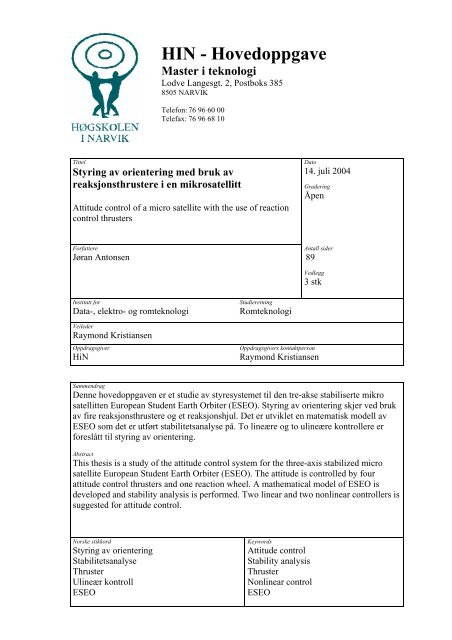
<strong>HIN</strong> - <strong>Hovedoppgave</strong><br />
Master i teknologi<br />
Lodve Langesgt. 2, Postboks 385<br />
8505 NARVIK<br />
Telefon: 76 96 60 00<br />
Telefax: 76 96 68 10<br />
Tittel<br />
Styring av orientering med bruk av<br />
reaksjonsthrustere i en mikrosatellitt<br />
Attitude control of a micro satellite with the use of reaction<br />
control thrusters<br />
Forfattere<br />
Jøran Antonsen<br />
Institutt for<br />
Data-, elektro- og romteknologi<br />
Veileder<br />
Raymond Kristiansen<br />
Oppdragsgiver<br />
HiN<br />
Studieretning<br />
Romteknologi<br />
Dato<br />
14. juli 2004<br />
Gradering<br />
Åpen<br />
Antall sider<br />
89<br />
Vedlegg<br />
3 stk<br />
Oppdragsgivers kontaktperson<br />
Raymond Kristiansen<br />
Sammendrag<br />
Denne hovedoppgaven er et studie av styresystemet til den tre-akse stabiliserte mikro<br />
satellitten European Student Earth Orbiter (ESEO). Styring av orientering skjer ved bruk<br />
av fire reaksjonsthrustere og et reaksjonshjul. Det er utviklet en matematisk modell av<br />
ESEO som det er utført stabilitetsanalyse på. To lineære og to ulineære kontrollere er<br />
foreslått til styring av orientering.<br />
Abstract<br />
This thesis is a study of the attitude control system for the three-axis stabilized micro<br />
satellite European Student Earth Orbiter (ESEO). The attitude is controlled by four<br />
attitude control thrusters and one reaction wheel. A mathematical model of ESEO is<br />
developed and stability analysis is performed. Two linear and two nonlinear controllers is<br />
suggested for attitude control.<br />
Norske stikkord<br />
Styring av orientering<br />
Stabilitetsanalyse<br />
Thruster<br />
Ulineær kontroll<br />
ESEO<br />
Keywords<br />
Attitude control<br />
Stability analysis<br />
Thruster<br />
Nonlinear control<br />
ESEO
<strong>Hovedoppgave</strong> vår 2004<br />
for<br />
Stud. Techn. Jøran Antonsen<br />
Styring av orientering med bruk av reaksjonsthrustere i en mikrosatellitt<br />
Den europeiske romfartsorganisasjonen ESA har satt i gang et samarbeidsprosjekt med<br />
universiteter over hele Europa. Prosjektet går under navnet Student Space Exploration &<br />
Technology Initiative (SSETI), og har som hensikt å opprette et nettverk av studenter og<br />
utdanningsinstitusjoner for distribuert design, konstruksjon og oppskyting av mikrosatellitter<br />
og andre romfartøy.<br />
Den første mikrosatellitten som utvikles i programmet er European Student Earth Orbiter<br />
(ESEO). Denne delen av prosjektet befinner seg på nåværende tidspunkt i fase B av utvikling.<br />
ESEO skal plasseres direkte i en geostasjonær bane av en Ariane 5 bærerakett i 2004.<br />
Oppgaven går i hovedsak ut på teoretiske analyser av stabilitet av ESEO, samt utvikling og<br />
simulering av robuste regulatorer for styring i tre akser. Konklusjoner skal underbygges med<br />
teoretisk analyse og simuleringer av dynamikk utført i MATLAB.<br />
Tekniske spesifikasjoner og krav for ESEO finnes i rapporten ESEO Phase-A Study Report<br />
utgitt av ESA.<br />
Deloppgaver:<br />
1. Gjør et litteraturstudium innen styring av orientering av mikrosatellitter og forstyrrelser.<br />
2. Utled en matematisk modell av ESEO med pådragsorganer, ut fra en spesifisert<br />
konfigurasjon av reaksjonsthrustere.<br />
3. Studer aktuatordynamikk for reaksjonsthrustere, og hvordan denne kan innvirke på styring<br />
av orientering.<br />
4. Foreslå regulatoralgoritmer for styring av satellitten i tre akser, og benytt simuleringer for<br />
å vise at regulatoralgoritmene overholder krav til nøyaktighet.<br />
5. Gjør vurderinger av størrelsesorden på forstyrrelser, og vurder de foreslåtte regulatorers<br />
evne til å undertrykke disse.<br />
6. Gi en algoritme for dumping av overflødig spinn i reaksjonshjul, og vis med simuleringer<br />
at denne fungerer tilfredstillende.
Som bakgrunn for oppgaven anbefales følgende litteratur (utgangspunkt):<br />
R. Kristiansen (2000): Attitude control of a micro satellite. Diplomoppgave, Institutt for<br />
Teknisk kybernetikk, NTNU<br />
M. J. Sidi (1997): Spacecraft Dynamics & Control. Cambridge University Press<br />
J. R. Wertz (1978): Spacecraft Attitude Determination and Control. D. Reidel Publishing<br />
Company, Dordrecht, Holland.<br />
Utleveringsdato: 28.01.2004<br />
Innleveringsdato: 14.07.2004<br />
Hovedveileder: Høgskolelektor Raymond Kristiansen, M.Sc<br />
Medveileder: Førsteamanuensis, Dr. Ing. Per J. Nicklasson<br />
<strong>Høgskolen</strong> i <strong>Narvik</strong><br />
Institutt for data, elektro og romteknologi<br />
Veileder<br />
(sign)
Preface<br />
The thesis is the concluding work of the Master of Science education provided by <strong>Narvik</strong> University College. It<br />
has been carried out at the Department of Computer Science, Electrical Engineering, and Space Technology. I<br />
would like to thank my advisor M.Sc Raymond Kristiansen and co-advisor Associate Professor Dr.ing. Per J.<br />
Nicklasson for their support, valuable advice, and interesting discussions during this work.<br />
Most of all I would like to thank my girl Gry for her love and support during the last five years. I would<br />
also like to thank my fellow students M.Sc Frank Robert Blindheim, M.Sc Aleksander L. Marthinussen and<br />
M.Sc Morten Topland for the many discussions during these last months.<br />
<strong>Narvik</strong> July 14 th 2004<br />
Jøran Antonsen<br />
iv
Abstract<br />
This thesis is a study of the attitude control system for the three-axis stabilized micro satellite European<br />
Student Earth Orbiter (ESEO). The satellite is regarded as a rigid body. The thesis introduces the satellite<br />
body dynamics relative to the orbit frame, where the angular velocity is represented relative to the orbit frame<br />
in stead of the inertial frame. This provides a model dependant of the same representation of angular velocity<br />
for both kinematics and dynamics.<br />
The attitude is controlled by four attitude control thrusters and one reaction wheel. A mathematical model of<br />
ESEO is developed and stability analysis is performed on both the linearized and the nonlinear model. The<br />
stability analysis of the linearized unactuated model concludes with an unstable satellite in the point where<br />
the body frame coincides with the orbit frame. Four equilibrium points is found with stability analysis on the<br />
nonlinear model, but none of them are where the body frame coincides with the orbit frame. Simulations of<br />
the unactuated satellite show that is unstable in the equilibrium point where the body frame coincides with the<br />
orbit frame.<br />
Four controllers is deduced for attitude control in this thesis, a PD controller, a Linear Quadratic Gaussian<br />
controller, a nonlinear controller based on feedback linearization, and a nonlinear controller based on Lyapunov.<br />
The controllers are compared against each other with respect to step response, power consumption and how<br />
robust they appear against disturbances. The controller based on feedback linearization is shown to have the<br />
fastest settling time whereas the PD controller has the second fastest settling time. The PD controller and the<br />
controller based on Lyapunov is shown to be most robust against disturbances and where the controller based<br />
on Lyapunov has the lowest power consumption. The LQG controller seems to be unstable with disturbances<br />
at several occasions.<br />
A Bang Bang controller with deadzone is used for control of the thrusters dynamic, but is not used when<br />
the attitude controllers is compared. A momentum dumper is deduced to prevent wheel saturation and also a<br />
suggestion for how to prevent wheel disturbance for the PD controller is shown. A reference trajectory is shown<br />
to be useful to keep the angular velocities low and to reduce the power consumption.<br />
v
CONTENTS 1<br />
Preface iv<br />
Abstract v<br />
Contents<br />
1 Introduction 4<br />
1.1 StudentSpaceExploration&TechnologyInitiative,SSETI ..................... 4<br />
1.1.1 EuropeanStudentEarthOrbiter(ESEO) ........................... 4<br />
1.1.2 SSETIExpress .......................................... 5<br />
1.1.3 EuropeanStudentMoonOrbiter(ESMO)........................... 5<br />
1.1.4 EuropeanStudentMoonRover(ESMR)............................ 5<br />
1.2 Other satellite missions ......................................... 5<br />
1.2.1 NCUBE.............................................. 5<br />
1.2.2 NSAT-1.............................................. 5<br />
1.2.3 Ørsted............................................... 6<br />
1.2.4 Rømer............................................... 6<br />
1.2.5 Proba1&2............................................ 6<br />
1.3 Outlineofthethesis ........................................... 7<br />
2 Mathematical background and notations 8<br />
2.1 The satellite ................................................ 8<br />
2.2 GeostationaryTransferOrbit(GTO).................................. 8<br />
2.3 Referenceframes ............................................. 11<br />
2.3.1 EarthCentredInertialframe(ECI)............................... 11<br />
2.3.2 Orbitframe(O) ......................................... 11<br />
2.3.3 Bodyframe(B).......................................... 12<br />
2.4 Notations ................................................. 12<br />
2.4.1 Vectors .............................................. 12<br />
2.4.2 Matrices.............................................. 12<br />
2.4.3 Pseudoinversematrices ..................................... 14<br />
2.5 RotationmatrixrepresentedinEulerangles.............................. 15<br />
2.6 RotationmatrixrepresentedinEulerparameters ........................... 16<br />
2.7 Stability definitions............................................ 17<br />
2.8 Liederivative ............................................... 19<br />
3 Mathematical modelling 20<br />
3.1 Dynamical satellite model . . . ..................................... 20<br />
3.2 Gravitationaltorque ........................................... 20<br />
3.3 Dynamicalmodelofthereactionwheel................................. 23<br />
3.4 Thrustertorque.............................................. 23<br />
3.5 Actuators ................................................. 26<br />
3.5.1 Fourthrustersandnoreactionwheel.............................. 27<br />
3.6 Disturbancetorque............................................ 28<br />
3.6.1 Gravitygradient ......................................... 28
CONTENTS 2<br />
3.6.2 Atmosphericdrag ........................................ 28<br />
3.6.3 SolarRadiationandSolarWind ................................ 29<br />
3.6.4 Internalnoise........................................... 29<br />
3.6.5 Thermal flexibility . . . ..................................... 29<br />
3.6.6 Sloshing.............................................. 29<br />
3.7 SolarPanels................................................ 30<br />
3.8 Dynamical model summary and simplifications ............................ 30<br />
3.9 Implementation.............................................. 31<br />
3.9.1 Eulerintegration......................................... 32<br />
3.9.2 ExplicitRungeKutta ...................................... 32<br />
4 Theoretical analysis 34<br />
4.1 Linearizationofthedynamicmodel................................... 34<br />
4.1.1 Linearizationofthekinematicequations............................ 34<br />
4.1.2 Linearizationoftherotationmatrix .............................. 34<br />
4.1.3 Linearizationoftheangularvelocity .............................. 34<br />
4.1.4 Linearizationofthegravitationaltorque............................ 35<br />
4.1.5 Linearizationofthereactionwheeltorque........................... 35<br />
4.1.6 Linearizationofthethrustertorque .............................. 35<br />
4.2 Completelinearizedmodel........................................ 36<br />
4.3 Stability of the linearized satellite model . . . ............................. 38<br />
4.4 Stability of the satellite - the Lyapunov approach ........................... 39<br />
4.5 Referencetrajectory ........................................... 42<br />
5 Controllers 44<br />
5.1 Thrusterallocation............................................ 44<br />
5.2 Pulsemodulation............................................. 44<br />
5.2.1 BangBangController ...................................... 44<br />
5.2.2 Pulse-WidthPulse-FrequencyModulator(PWPFM)..................... 44<br />
5.2.3 Pulse-WidthModulator(PWM) ................................ 45<br />
5.3 LinearControl .............................................. 45<br />
5.3.1 PDcontroller........................................... 45<br />
5.3.2 PDcontrollerwithwheelcompensation ............................ 47<br />
5.3.3 LinearQuadraticGaussian(LQG)controller ......................... 47<br />
5.4 NonlinearControl ............................................ 48<br />
5.4.1 NonlinearcontrolbyLyapunov................................. 49<br />
5.4.2 NonlinearcontrolbyFeedbackLinearization.......................... 50<br />
5.5 Momentumdumpingcontroller ..................................... 53<br />
6 Simulation and results 55<br />
6.1 Unactuated satellite ........................................... 55<br />
6.2 Stepresponse............................................... 56<br />
6.3 Disturbance................................................ 60<br />
6.3.1 Disturbanceonthemeasurements ............................... 60<br />
6.3.2 Disturbanceontheactuators .................................. 64<br />
6.3.3 Disturbanceonthemeasurementsandtheactuators ..................... 68
CONTENTS 3<br />
6.4 Summaryofresults............................................ 72<br />
6.5 BangBangcontroller........................................... 75<br />
6.6 Momentumdumpingcontroller ..................................... 76<br />
6.7 Wheeldisturbancecompensation .................................... 76<br />
6.8 Powerconsumption............................................ 77<br />
6.9 Referencetrajectory ........................................... 81<br />
7 Discussion 82<br />
7.1 Theoreticalanalysis ........................................... 82<br />
7.2 Simulations ................................................ 82<br />
7.2.1 Unactuated satellite . . ..................................... 82<br />
7.2.2 Stepresponse........................................... 83<br />
7.2.3 Disturbance............................................ 83<br />
7.2.4 BangBangcontroller ...................................... 84<br />
7.2.5 Momentumdumpingcontroller................................. 84<br />
7.2.6 Wheeldisturbancecompensation................................ 84<br />
7.2.7 Powerconsumption........................................ 84<br />
7.2.8 Referencetrajectory ....................................... 85<br />
8 Concluding Remarks and Recommendations 86<br />
8.1 Conclusion ................................................ 86<br />
8.2 Recommendationsforfuturework ................................... 87<br />
9 Bibliography 88<br />
A Notations 90<br />
A.1 Vectricesanddyadics........................................... 90<br />
B Simulations 91<br />
C Matlab sourcecode 98
1 INTRODUCTION 4<br />
1 Introduction<br />
This thesis is a study of the attitude control system for the micro satellite European Student Earth Orbiter<br />
(ESEO). The satellite is three-axis stabilized by the use of four attitude control thrusters and one reaction<br />
wheel. ESEO is currently being deigned and constructed by European students, members of the Student Space<br />
Exploration & Technology Initiative (SSETI) and is planned to be launched late 2005. The satellites main<br />
objectiveistotakepicturesoftheearthandthemoon,and requires an attitude control system to be able to<br />
rotate to desired positions.<br />
1.1 Student Space Exploration & Technology Initiative, SSETI<br />
Student Space Exploration & Technology Initiative (SSETI) was founded by the support of the European Space<br />
Agency (ESA) in the year 2000. The main objective of the SSETI is stated as (ESEO Phase A Study Report,<br />
2001)<br />
To create a network of students, educational institutions and organizations (on the Internet) to perform the<br />
distributed design, construction and launch of (micro)-satellites and other spacecraft (s/c).<br />
The objectives are reached when a spacecraft is design, build and launched by a significant number of European<br />
students in a highly distributed way. The completion of this project objective is independent of a mission<br />
success or failure. More about SSETI ongoing and future missions can be found at the SSETI homepage,<br />
http://www.sseti.org/.<br />
1.1.1 European Student Earth Orbiter (ESEO)<br />
• The SSETI micro satellite (ESEO), is a micro satellite designed, built and operated as the first SSETI<br />
mission by the European students working in the network of participating universities. The ESEO is the<br />
first SSETI project which started late 2000 and defined as mission one. The main mission objectives for<br />
the ESEO is as stated (SSETI Phase A Study Report, 2001)<br />
• Take picture of impact on public order to increase the interest of European students in space missions.<br />
• Take one picture of the moon to increase the enthusiasm of students to reach the Moon on future missions.<br />
• Test and qualify a star-tracker developed from a commercial device.<br />
• Deploy integrated radiation dosimeters within OBDH nodes and central "PC box" to monitor radiation<br />
dosage during the mission.<br />
• Test and qualify a propulsion system for orbit maneuvers and future moon missions, by putting the spacecraft<br />
in a 12-hour orbit.<br />
• No life critical failures should occur in the first 28 days of the mission. End of mission is when it is not<br />
possible to communicate with the spacecraft anymore.<br />
These objectives shall be reached by means of a spacecraft system and related instruments and payload. The<br />
mission is defined as successful by maintaining the satellite in GTO for at least 28 days, testing the essential<br />
subsystems and performing the simple science payload experiments. The satellites is set to launched from Korou<br />
late 2005.
1 INTRODUCTION 5<br />
1.1.2 SSETI Express<br />
SSETI Express is a micro satellite where the work started in December 2003 and defined by SSETI as mission<br />
zero. This is a satellite which uses some of the already designed subsystems developed for the ESEO. The<br />
satellite is planned to be launched early 2005.<br />
1.1.3 European Student Moon Orbiter (ESMO)<br />
The European Student Moon Orbiter (ESMO) is the future mission two of SSETI. A feasibility study of the<br />
ESMO started in 2004, but no final objectives have been defined yet. The main idea for ESMO is to use if<br />
possible some of the knowledge and hardware from the ESEO mission.<br />
1.1.4 European Student Moon Rover (ESMR)<br />
The European Student Moon Rover (ESMR) is another future mission three of the SSETI which not yet has<br />
started, but where the idea is to land the ESMR on the moon.<br />
1.2 Other satellite missions<br />
1.2.1 NCUBE<br />
The Norwegian student satellite NCUBE is an experimental spacecraft which is developed and built by students<br />
from four Norwegian universities. The project was initiated by the Norwegian Space Centre with support from<br />
Andøya Rocket Range, Norway. The main mission of the satellite is to demonstrate ship traffic surveillance<br />
from a satellite in LEO using the maritime Automatic Identification System (AIS). The AIS system is based<br />
on VHF transponders located onboard ships. These transponders broadcast the position, speed, heading and<br />
other relevant information from the ships at regular time intervals. The main objective of the satellite is to<br />
receive, store and retransmit at least one AIS-message from a ship. Another objective of the satellite project is<br />
to demonstrate reindeer herd monitoring from space by equipping a reindeer with an AIS transponder during<br />
a limited experimental period. This part of the project is conducted by the Norwegian Agriculture University<br />
(NLH). A third objective is to demonstrate efficient attitude control system using a combination of passive<br />
gravity gradient stabilization and active magnetic torquers. It is possible to control the attitude of the satellite<br />
such that the nadir surface points towards the earth within limits of ±10 ◦ ,whichissufficient for antenna<br />
pointing. For more information, see e.g. Rise et al(2003) and the NCUBE hompage at http://128.39.102.180/.<br />
1.2.2 NSAT-1<br />
The development of the proposed three-axis stabilized Norwegian micro satellite NSAT-1 has been ongoing for<br />
several years. The satellite is intended to fly in a low earth orbit at 600 km altitude with the purpose of locating<br />
ships at sea. The satellite should be able to locate a ship within a few hundred meters, and high demands are<br />
placed on the attitude control system. The satellite control system will consist of a composition of a gravity<br />
boom, reaction wheels and magnetic coils.<br />
Several people have performed studies on NSAT-1. More information about the NSAT-1 can be found in<br />
(Kristiansen, 2000) and (Kyrkjebø, 2000). Kristiansen (2000) performed several simulations of the attitude<br />
control system of the NSAT-1. Disturbances on the actuators where added to be 20%, and showed that the<br />
proposed controllers where robust and handled the disturbances quite well.
1 INTRODUCTION 6<br />
1.2.3 Ørsted<br />
The Ørsted satellite is a 62kg Danish micro satellite, and was launched from California on January 8, 1999. The<br />
main purpose of the Ørsted satellite has been to provide a precise global mapping of the Earth’s magnetic field.<br />
The satellite evolves the Earth in an elliptic orbit of heights between 600 and 850 km. The attitude controls<br />
system consists of three orthogonal magnetic coils and a gravity boom. Flight results and experience from the<br />
Ørsted attitude control system can be found in (Bak, T. et al, 1999). For more information about the Ørsted<br />
mission, see the Ørsted homepage on the internet at<br />
http://dmiweb.dmi.dk/fsweb/projects/oersted/homepage.html.<br />
1.2.4 Rømer<br />
Rømer is the next Danish micro satellite mission scheduled to be launched in 2005 - 2006 from Plesetsk Cosmodrome<br />
in Russia. It has the same dimensions as the ESEO but the weight is 85 kg. The satellite is scheduled<br />
to be launched into a Molniya orbit in which one orbit takes approximately 12 hours, the same as for the ESEO<br />
GTO orbit. The scientific experiments implemented are Measuring Oscillations in Nearby Stars (MONS) with<br />
the primary science objective of observing 25 nearby, solar like stars by measuring tiny oscillations in intensity<br />
and color by precision photometry.<br />
For attitude control the Rømer satellite is equipped with a tetrahedron configuration of Wide Angle Telescopes<br />
for Cosmic Hard x-rays (WATCH), that serves the dual purpose of x-ray detectors and momentum<br />
wheels for short term attitude control (seconds to hours). Also a set of magnetic coils or rods for long term<br />
control (days) and momentum dumping is used in addition to the WATCH for attitude control. A proposed<br />
nonlinear attitude controller for the Rømer satellite based on feedback linearization can be found in (Jensen and<br />
Wi´sniewski, 2001). Another passivity based nonlinear attitude controller suggested for the Rømer satellite can<br />
be found in (Quottrup et al, 2000). More information and documents about the Rømer mission can be found<br />
at the Danish Space Research Institute (DSRI) at http://www.dsri.dk/.<br />
1.2.5 Proba 1 & 2<br />
The Proba-1 satellite was the first micro satellite launched by ESA. It has a weight of 94kg and has the same<br />
dimensions as ESEO, 60x60x80 cm. The name Proba comes from the Project for On-board Autonomy. Proba-1<br />
was launched from Antrix (India) 22 October, 2001, initially for a one-year mission. The satellite was injected<br />
directly into its final polar, sun-synchronous orbit at an altitude of 817km, 98.7 degrees inclination. There is<br />
no on-board propulsion because of only 2 degrees orbital drift per year. The satellite is three-axis stabilized<br />
by means of attitude provided by a star tracker and by on-board control through a set of reaction wheels and<br />
magnetic coils.<br />
ESA’s second micro satellite, Proba-2, is under development for launch early in 2006. It will have the same<br />
dimensions as Proba-1. Proba 2 will offer increased miniaturization and integration of avionics, improved performance,<br />
and with more resources allocated to payloads. The satellite uses its main instrument called SWAP<br />
to watch the Sun and make detailed images of the solar atmosphere once a minute, by the light of energetic<br />
ultraviolet rays. Proba-2 will give early warnings of eruptions on the Sun that provoke stormy weather throughout<br />
the solar system.<br />
The Proba missions are a part of an overall effort to promote technological missions using small spacecraft.
1 INTRODUCTION 7<br />
For more information about the Proba missions, see the ESA website at<br />
http://www.esa.int/SPECIALS/Proba_web_site/index.html.<br />
1.3 Outline of the thesis<br />
This M.Sc thesis is organized as follows:<br />
Mathematical background information and notation used in this thesis is described in Chapter 2. This includes<br />
parameters and definitions of the space environment, in addition to reference frames and conversion between<br />
these and stability definitions.<br />
A complete mathematical model of the satellite with all its components is deduced in Chapter 3. A description<br />
of the actuator configuration and different disturbance torques is mentioned.<br />
Chapter 4 consists of a theoretical analysis where the dynamical model is linearized and stability analysis<br />
is performed both on the linear and nonlinear model. The principal of a reference model is also shown in this<br />
chapter.<br />
Chapter 5 is dedicated to control strategies for the satellite where different attitude controllers are deduced<br />
including a momentum dumping controller and a Bang Bang controller.<br />
Simulation of the theoretical control strategies is shown in Chapter 6, for the main purpose of illustrating<br />
the satellite step response and the robustness of the controllers and to substantiate the result found in the<br />
theoretical analysis. The power consumption of each controller is investigated. The motivation for using a<br />
reference model is illustrated and the need for angular momentum dumping from the reaction wheel by using<br />
thrusters.<br />
A discussion of the theoretical analysis and the results from simulations is done in Chapter 7.<br />
Finally Chapter 8 includes conclusions made from the work presented in this thesis, together with some<br />
recommendations for future work.
2 MATHEMATICAL BACKGROUND AND NOTATIONS 8<br />
2 Mathematical background and notations<br />
2.1 The satellite<br />
The Student Space Exploration & Technology Initiative, SSETI is building a micro satellite called the European<br />
Student Earth Orbiter, ESEO with the dimension 60 × 60 × 80 cm3 , and a total mass of approximately 120<br />
kg. For Attitude and Orbit Control System (AOCS), the ESEO uses one reaction wheel in y-axis controlling<br />
the pitch movement, four thrusters for attitude control (from here on called Attitude Control System thruster<br />
or ACS thruster), one main Orbit Control thruster (from here on called Orbit Control System thrusters or<br />
OCS thrusters) for orbital manoeuvres, and additional four Reaction Control Thrusters (from here on called<br />
Reaction Control System thruster or RCS thruster) used to correct orbital manoeuvres since the OCS thrust<br />
vector might not go through the centre of mass. The RCS thrusters are also used as a redundancy for the ACS<br />
thrusters. This thesis is about the attitude control system (ACS) which includes the ACS thrusters and the<br />
reaction wheel. The required attitude accuracy for ESEO is 1◦ in x-axis and y-axis, and 5◦ in the z-axis (ESEO<br />
phase B document). The satellite in this thesis is assumed to be a rigid body, with an inertia matrix<br />
⎡<br />
I = ⎣ Ix<br />
0<br />
0<br />
Iy<br />
0<br />
0<br />
⎤ ⎡<br />
⎦ = ⎣<br />
0 0 Iz<br />
2.2 Geostationary Transfer Orbit (GTO)<br />
4.3500 0 0<br />
0 4.3370 0<br />
0 0 3.6640<br />
⎤<br />
⎦ kgm 2<br />
The ESEO is expected to be launched by Ariane 5 from Kourou into a Geostationary Transfer Orbit (GTO).<br />
However, the final orbital parameters are not yet defined. Estimated orbital data for the ESEO is listed in<br />
Table 2.1 (ESEO phase B document)<br />
Table 2.1. Orbital parameters<br />
Apogee 35843.369 km<br />
Perigee 252.560 km<br />
Semimajor axis 24421.104 km<br />
Eccentricity 0.7285<br />
Inclination 7 ◦<br />
A graphical description of the GTO is shown in Figure 2.1where perigee is the point in the orbit where the<br />
apogee<br />
GTO<br />
equator<br />
Figure 2.1: Geostationary Transfer Orbit.<br />
perigee<br />
distance to earth centre is minimum and apogee is the point in the orbit with the maximum distance. In any<br />
(2.1)
2 MATHEMATICAL BACKGROUND AND NOTATIONS 9<br />
given orbit the intersection of the orbit plane and the reference plane through the centre of mass of the Earth is<br />
the line of nodes. The ascending node of the satellite is the point where it crosses the equatorial plane travelling<br />
from south to north. Similar, the descending node is where it crosses the equatorial plane travelling from north<br />
to south. The nodes are shown in Figure 2.2. The eccentricity e defines the shape of the orbit ellipse as the<br />
ratio<br />
r<br />
a2 − b2 e =<br />
(2.2)<br />
a<br />
where a and b is the semimajor and semiminor axis, which is half the long and short axis in an ellipse, respectively.<br />
For circular orbits, the eccentricity is e =0because the semimajor and the semiminor axis is of the same length.<br />
Similar, the apogee and perigee of the orbit will be the same in a circular orbit.<br />
Earth orbit<br />
direction<br />
North<br />
South<br />
Descending<br />
node<br />
Ascending<br />
node<br />
Satellite orbit<br />
direction<br />
Equatorial<br />
plane<br />
Figure 2.2: Ascending and descending nodes in an orbit.<br />
The nominal duration of this mission is 28 days. During this period the ESEO will spend 10 days in GTO<br />
phase, and then ESEO will perform manoeuvres in order to reach a suitable orbit for suffering a natural de-orbit.<br />
The angular velocity in the orbit, is given as (Sidi, 1997)<br />
r<br />
µ<br />
ωo =<br />
(2.3)<br />
R3 C<br />
where µ = G·mearth =3.986·1014Nm2 /kg and G =6.669·10−11m3 /kg2 is the universal constant of gravitation,<br />
mearth =5.97·1024 ¯<br />
kg is the total Earth mass and R = ¯ ¯<br />
R¯<br />
is the distance from the centre of Earth to the centre<br />
of the satellite. Since the ESEO is in a GTO, the distance from Earth centre to the satellite centre will not be<br />
constant. The distance RC is given as (Sidi, 1997)<br />
RC = a(1 − e2 )<br />
(2.4)<br />
1+e cos θ<br />
where a is the semimajor axis, e is the eccentricity, and θ is the true anomaly defined as the angle between the<br />
major axis pointing to the perigee and the radius vector from the centre of earth to the satellite. True and<br />
eccentric anomaly θ and ψ is shown in Figure 2.3. It can be shown that (Sidi , 1997)<br />
cos ψ =<br />
e +cosθ<br />
1+cosθ<br />
(2.5)
2 MATHEMATICAL BACKGROUND AND NOTATIONS 10<br />
and by substituting cos θ from (2.5) into (2.4),<br />
and by using Kepler’s time equation (Sidi, 1997)<br />
apogee<br />
orbit<br />
RC = a (1 − e cos ψ) (2.6)<br />
b<br />
a<br />
O<br />
ψ<br />
r<br />
θ<br />
F<br />
perigee<br />
Figure 2.3: True and eccentric anomalies.<br />
2π<br />
tM<br />
T =(t− tp) n = M = ψ − e sin ψ (2.7)<br />
where tM = t − tp is the time elapsed from the last passage at perigee, n = 2π<br />
T is the mean motion, and M is the<br />
mean anomaly. Equation (2.7) is not solvable in closed form with respect to ψ, itmustbesolvednumerically.<br />
A solution of (2.7) in the form of trigonometric series was developed by Lagrange as<br />
ψ = M +2<br />
∞X<br />
n=1<br />
1<br />
n Jn (ne)sin(nM) (2.8)<br />
where Jn is a Bessel function of the first kind of order n 1 . A simple numeric procedure based on successive<br />
approximations may be used to find ψ in an elliptic orbit (e
2 MATHEMATICAL BACKGROUND AND NOTATIONS 11<br />
Rc [m]<br />
wo [rad/s]<br />
x 107<br />
4.5<br />
4<br />
3.5<br />
3<br />
2.5<br />
2<br />
1.5<br />
1<br />
Distance from center of earth to center of satellite<br />
0 0.5 1 1.5 2 2.5 3 3.5 4 4.5<br />
x 10 4<br />
0.5<br />
x 10-3<br />
1.2<br />
1<br />
0.8<br />
0.6<br />
0.4<br />
0.2<br />
Satellite angular velocity relative to earth<br />
0 0.5 1 1.5 2 2.5 3 3.5 4 4.5<br />
x 10 4<br />
0<br />
Figure 2.4: Satellite angular velocity and distance from the center of earth to the satellite.<br />
2.3 Reference frames<br />
Without reference points and frames it is not possible to model positions or motions of a spacecraft. Only the<br />
frames that are of importance for the modelling of a satellite like the ESEO is presented. For earth orbiting<br />
satellites the rotation of the earth can often be neglected. Under these circumstances the earth itself becomes<br />
the inertial reference.<br />
2.3.1 Earth Centred Inertial frame (ECI)<br />
For satellites it is common to define an inertial coordinate system with the centre of mass of the earth as its<br />
origin (Earth Centred Inertial, ECI frame) and whose direction in space is fixed relative to the solar system 2 .<br />
The Zi axis is directed from the centre of earth to the celestial north pole. The Xi axis is directed to the vernal<br />
equinox, the point where the ecliptic, or the plane of the Earth’s orbit round the Sun, crosses the Equator from<br />
south to north. Last the Yi axis together with the Xi axis make the equatorial plane of the Earth, which is<br />
perpendicular to the earth’s axis of rotation. Figure 2.5 shows a graphical description of the ECI frame.<br />
2.3.2 Orbit frame (O)<br />
For earth orbiting satellites, it is most convenient to define a reference frame called the orbit frame. The<br />
orbit frame has its base point at the centre of mass and has the vectors XO, YO, andZO. The XO-axis is<br />
directed forward in the travelling direction of the satellite, ZB is directed to the centre of earth, and YO- axis<br />
is perpendicular to the orbit plane and completes a right-hand orthogonal system.<br />
2 This is actually not a inertial frame because the ECI system moves slowly relative to the stars. Today, it is common to classify<br />
the stars relative to the ECI for the year 2000 (Sidi, 1997).
2 MATHEMATICAL BACKGROUND AND NOTATIONS 12<br />
2.3.3 Body frame (B)<br />
Figure 2.5: Earth Centered Inertial frame.<br />
A rigid body can be represented by the so-called body frame. This frame is important for modelling location<br />
and orientation of a satellite under study. Its base point also coincides with the centre of mass, and the base<br />
vectors XB, YB, andZB are aligned with the principal axes of the moment of inertia tensor to simplify the<br />
kinetic equations. Rotation about the axis XB, YB, andZB is defined as roll, pitch, andyaw respectively. The<br />
body frame together with the orbit frame is shown in Figure 2.6.<br />
2.4 Notations<br />
2.4.1 Vectors<br />
A vector independent from any frame will be denoted v, and coordinate vectors represented in a frame will be<br />
denoted with a bold font and a superscript to indicate the frame. Then vB is a vector represented in the body<br />
frame. Angular velocity vectors are denoted similar to other vectors, but with additional subscript to state<br />
which frame that has angular velocity and relative to what frame. The vector ωB BI denotes the angular velocity<br />
of the body frame relative to the inertial frame expressed in body frame.<br />
2.4.2 Matrices<br />
Matrices will be denoted similar to vectors with bold typing and a superscript to indicate the frame that matrices<br />
are represented in for dependent matrices and with an arrow above the matrix for independent ones. The unity<br />
matrix will be denoted as 1. Normally it is denoted as I, butI is in this case the notation for the moment of<br />
inertia for the satellite. The rotation matrix, which transforms a coordinate vector from a system A to system
2 MATHEMATICAL BACKGROUND AND NOTATIONS 13<br />
B, is denoted R A B<br />
Orbit<br />
YO<br />
YB<br />
Satellite<br />
ZO<br />
To Earth<br />
Center<br />
ZB<br />
Figure 2.6: Body and orbit frame.<br />
v A = R A Bv B<br />
This can be used to describe the orientation of a satellite relative to the orbit frame, RB O<br />
R B O =<br />
⎡<br />
⎤<br />
⎦ (2.12)<br />
⎣ c11 c12 c13<br />
c21 c22 c23<br />
c31 c32 c33<br />
where the elements cij is called directional cosines, and as vectors they are named c1, c2, andc3<br />
⎡ ⎤<br />
⎡ ⎤<br />
⎡ ⎤<br />
c1 = ⎦ c2 = ⎦ c3 = ⎦ (2.13)<br />
⎣ c11<br />
c21<br />
c31<br />
⎣ c12<br />
c22<br />
c32<br />
XB<br />
⎣ c13<br />
c23<br />
The rotation matrix RB O is orthogonal, which makes the vectors orthonormal, and<br />
c1 × c2 = c3 c2 × c3 = c1 c1 × c3 = c2 (2.14)<br />
The rotation matrix RB A has the property<br />
R A ¡ ¢T B<br />
B RA = 1 ⇐⇒<br />
A<br />
RB = ¡ R B¢−1 ¡ ¢T B<br />
A = RA this means that its inverse equals its transpose. This can be derived as (Egeland and Gravdahl, 2003)<br />
˙R A B<br />
c33<br />
XO<br />
(2.15)<br />
¡ ¢ ³<br />
BT A<br />
RA + R ˙R B<br />
B ´ T<br />
A =0 (2.16)
2 MATHEMATICAL BACKGROUND AND NOTATIONS 14<br />
By defining a matrix S as<br />
S , ˙R A ¡ ¢ B<br />
B RA and inserting this into (2.16), the derived expression turns into<br />
S + S T =0 ⇐⇒ S = −S T<br />
(2.17)<br />
(2.18)<br />
which implies that the matrix S is skew-symmetrical, and therefore it must exist a vector given as ωA AB =<br />
£ ¤ T<br />
ω1 ω2 ω3 in such a way that<br />
S ¡ ω A ¢<br />
AB =<br />
⎡<br />
⎣ 0 −ω3 ω2<br />
ω3 0 −ω1<br />
−ω2 ω1 0<br />
⎤<br />
⎦ (2.19)<br />
where the coordinate vector ωA AB represents the angular velocity of frame A relative to frame B expressed in<br />
frame A. The matrix S ¡ ωA ¢<br />
AB expresses the cross product of two vectors as<br />
S ¡ ω A ¢ A<br />
AB RB = ω A AB × R A B<br />
(2.20)<br />
This relation implies that<br />
S ¡ ω A ¢ A<br />
AB RB = −R A BS ¡ ω A ¢<br />
AB<br />
The derived rotation matrix ˙R A B can now be solved using (2.17) as<br />
˙R A B = S ¡ ω A ¢ A<br />
AB RB = R A BS ¡ ω B ¢<br />
AB<br />
2.4.3 Pseudo inverse matrices<br />
(2.21)<br />
(2.22)<br />
Pseudo inverse is a method to find the inverse of a non square matrix. A system matrix has to have either<br />
existence or uniqueness properties to be invertible, defined as (Strang, 1988)<br />
Definition 2.1<br />
Existence: The system Ax = b has at least one solution x for every b if and only if the columns span R m ;then<br />
r = m. In this case there exists an n by m right-inverse A ` such that AA ` =1m, the identity matrix of order<br />
m. This is possible only if m ≤ n.<br />
Definition 2.2<br />
Uniqueness: The system Ax = b has at most one solution x for every b if and only if the columns are linearly<br />
independent; then r = n. In this case there exists an n by m left-inverse A a such that A a A =1n, theunity<br />
matrix of order n. Thisispossibleonlyif m ≥ n.<br />
There are two simple formulas of pseudo inverse, left and right inverses, if they exist<br />
A a = ¡ A T A ¢−1 T<br />
A and A ` ³<br />
T<br />
= A AA T ´ −1<br />
(2.23)<br />
Then A a A = 1 and AA ` = 1. It is however not always that A T A,andAA T are actually invertible. A T A<br />
has an inverse only if the rank is n, andAA T has an inverse when the rank is m.
2 MATHEMATICAL BACKGROUND AND NOTATIONS 15<br />
2.5 Rotation matrix represented in Euler angles<br />
The Euler angle rotation is defined as successive angular rotation about three orthogonal frame axes. The<br />
rotation from the orbit frame to the body frame can be expressed as a rotation first about the z axis then about<br />
y, and x axis with the angles ψ, θ, andφrespectively. This rotation is shown in Figure 2.7, and can be expressed<br />
as (Egeland, 1993)<br />
(2.24)<br />
R O B = Rz,ψRy,θRx,φ<br />
where Rz,ψ, Ry,θ, andRx,φ is the unity rotation<br />
⎡<br />
Rz,ψ = ⎣<br />
cψ −sψ 0<br />
sψ cψ 0<br />
0 0 1<br />
⎤ ⎡<br />
⎦ Ry,θ = ⎣<br />
cθ 0 sθ<br />
0 1 0<br />
−sθ 0 cθ<br />
⎤ ⎡<br />
⎦ Rx,φ = ⎣<br />
1 0 0<br />
0 cφ −sφ<br />
0 sφ cφ<br />
⎤<br />
⎦ (2.25)<br />
where s(·)and c(·) is the same as sin(·) and cos(·) respectively just to simplify the notation. With the help of<br />
the unity rotations, RO B can be written as<br />
⎡<br />
R O B = ⎣<br />
cψcθ cψsθsφ − sψcφ cψcφsθ + sψsφ<br />
sψcθ sψsθsφ + cψcφ sψsθcφ − cψsφ<br />
−sθ cθsφ cθcφ<br />
⎤<br />
⎦ (2.26)<br />
The rotation matrix RO B becomes the unity matrix 1 if the angles φ = θ = ψ =0, which implies that no rotation<br />
has occurred. The rotation matrix RO B can be described as a rotation by an angle θ about a unit vector k where<br />
RO B is given by (Egeland, 1993)<br />
R O B =cosθ1 + S ¡ k B¢ sin θ + k B ¡ k B¢T (1 − cos θ) (2.27)<br />
and inserting<br />
S 2 ¡ k B¢ = k B ¡ k B¢T ¡ B<br />
− k ¢T B B<br />
k 1 = k ¡ k B¢T − 1 (2.28)<br />
gives the equation<br />
R O B = 1 + S ¡ k B¢ sin θ + S 2 ¡ k B¢ (1 − cos θ) (2.29)<br />
This implies that the directional cosines in (2.13) enters the form<br />
⎡<br />
c1 = ⎣ cψcθ<br />
⎤<br />
cψsθsφ − sψcφ ⎦<br />
⎡<br />
c2 = ⎣<br />
cψcφsθ + sψsφ<br />
sψcθ<br />
⎤<br />
sψsθsφ + cψcφ ⎦<br />
⎡<br />
c3 = ⎣<br />
sψsθcφ − cψsφ<br />
−sθ<br />
⎤<br />
cθsφ ⎦ (2.30)<br />
cθcφ<br />
This parameter representation has its disadvantage in the singularity problem. Consider for instance that,<br />
θ = ± π<br />
2 , which gives the rotational matrix RO B<br />
⎡<br />
R O B = ⎣<br />
0 cψsφ − sψcφ cψcφ + sψsφ<br />
0 sψsθsφ + cψcφ sψsθcφ − cψsφ<br />
−1 0 0<br />
⎤<br />
⎦ (2.31)<br />
which is singular. This implies that there will be no inverse solution to this problem, and the rotation can not<br />
be found.
2 MATHEMATICAL BACKGROUND AND NOTATIONS 16<br />
YB<br />
θ<br />
ZB<br />
Satellite<br />
cm<br />
ψ<br />
Figure 2.7: Description of a rotation roll, pitch, and yaw with the angles φ, θ, andψ respectively.<br />
2.6 Rotation matrix represented in Euler parameters<br />
Euler parameters are a four parameter representation and have no singularity. The Euler parameters are defined<br />
in terms of the angle-axis parameter θ and k, andaregivenbythescalarηand the vector ε defined by (Egeland<br />
and Gravdahl, 2003)<br />
q , £ ¤ T<br />
η ε1 ε2 ε3<br />
(2.32)<br />
where<br />
µ <br />
θ<br />
η =cos<br />
2<br />
and ε = £ ε1 ε2 ε3<br />
where ε and k is represented in the body frame. Note that<br />
η 2 + ε T ε =cos 2<br />
µ θ<br />
2<br />
<br />
+sin 2<br />
φ<br />
¤ T = k sin<br />
XB<br />
µ <br />
θ<br />
2<br />
(2.33)<br />
µ <br />
θ<br />
=1 (2.34)<br />
2<br />
The Euler parameter product between vectors q1 = £ η1 εT 1<br />
¤ T<br />
and q2 = £ η2 εT (Egeland and Gravdahl, 2003)<br />
2<br />
∙<br />
η1<br />
q , q1q2 =<br />
ε1<br />
¸ ∙<br />
η2<br />
ε2<br />
¸ ∙<br />
η<br />
=<br />
1η2 − εT 1 ε2<br />
η1ε2 + η2ε1 + S (ε1) ε2<br />
¸<br />
¤ T can be found as<br />
(2.35)
2 MATHEMATICAL BACKGROUND AND NOTATIONS 17<br />
The rotation matrix RO B can be written as (Egeland, 1993)<br />
R O B = Rk,θ = Rη,ε , ¡ η 2 − ε T ε ¢ 1 +2εε T +2ηS (ε) (2.36)<br />
= ¡ 2η 2 − 1 ¢ 1 +2εε T +2ηS (ε) (2.37)<br />
= ¡ 1 − 2ε T ε ¢ 1 +2εε T +2ηS (ε) (2.38)<br />
and by using (2.28) and (2.36) gives<br />
R O B = 1 +2ηS (ε)+2S 2 (ε) (2.39)<br />
whichcanbeexpressedincomponentsas<br />
R O ⎡<br />
B = ⎣ 1 − 2 ¡ ε2 2 + ε2 ¢<br />
3<br />
2(ε1ε2 + ηε3)<br />
2(ε1ε2 − ηε3)<br />
1−2 2(ε1ε3 + ηε2)<br />
¡ ε2 1 + ε2 2(ε1ε3 − ηε2)<br />
¢<br />
3<br />
2(ε2ε3 + ηε1)<br />
2(ε2ε3 − ηε1)<br />
1−2 ¡ ε2 1 + ε2 ⎤<br />
⎦<br />
¢<br />
2<br />
(2.40)<br />
The inverse rotation RO B can now be found as<br />
R B O = 1 − 2ηS (ε)+2S2 (ε) (2.41)<br />
and from (2.15) the inverse rotation matrix is the same as the transpose rotation matrix, hence<br />
R B O = ¡ R O ⎡<br />
¢T<br />
B = ⎣ 1 − 2 ¡ ε2 2 + ε2 ¢<br />
3<br />
2(ε1ε2 − ηε3)<br />
2(ε1ε2 + ηε3)<br />
1−2 2(ε1ε3−ηε2) ¡ ε2 1 + ε2 2(ε1ε3 + ηε2)<br />
¢<br />
3<br />
2(ε2ε3−ηε1) 2(ε2ε3 + ηε1)<br />
1−2 ¡ ε2 1 + ε2 ¢<br />
2<br />
⎤<br />
⎦ (2.42)<br />
The directional cosines from (2.30) can now be expressed in Euler parameters as<br />
⎡<br />
c1 = ⎣ 1 − 2 ¡ ε2 2 + ε2 ¢ ⎤<br />
3<br />
2(ε1ε2 − ηε3) ⎦<br />
2(ε1ε3 + ηε2)<br />
⎡<br />
c2 = ⎣ 2(ε1ε2 + ηε3)<br />
1 − 2 ¡ ε2 1 + ε2 ⎤<br />
¢<br />
⎦<br />
3<br />
2(ε2ε3 − ηε1)<br />
⎡<br />
c3 = ⎣ 2(ε1ε3 − ηε2)<br />
2(ε2ε3 + ηε1)<br />
1 − 2 ¡ ε2 1 + ε2 ⎤<br />
⎦<br />
¢<br />
2<br />
(2.43)<br />
The kinematic equation for the Euler parameters can be expressed as (Egeland and Gravdahl, 2003)<br />
˙η = − 1<br />
2 εT ω B BO<br />
2.7 Stability definitions<br />
˙ε = 1<br />
2 [η1 + S (ε)] ωB BO<br />
(2.44)<br />
(2.45)<br />
For stability analysis of the satellite system, Lyapunov theory is a suitable choice. Definitions and theorems in<br />
this section is inspired by (Slotine and Li, 1991). Lyapunovs method is often used to investigate the stability in<br />
nonlinear systems. Lyapunovs method is used in this thesis where the idea is to define a continuous derivable,<br />
positive definite function which reflects the energy in the system. This function is called the Lyapunov Candidate<br />
Function (LCF). If the initial energy in the system dissipates, the system can be regarded as stable. In Lyapunov<br />
analysis of non-autonomous nonlinear systems of the form<br />
˙x = f (x, t) (2.46)
2 MATHEMATICAL BACKGROUND AND NOTATIONS 18<br />
where f is a n × 1 nonlinear vector function, and x is the n × 1 state vector, some different concepts of functions<br />
has to be defined. The first is the concept of equilibrium points, which are definedaspointswherethesystem<br />
states can stay forever. This implies that the state derivative is equal to zero, ˙x = 0. Many of the stability<br />
problems are naturally formulated with respect to equilibrium points.<br />
Definition 2.3<br />
A state x ∗ is an equilibrium state or equilibrium point of the system if once x is equal to x ∗ , it remain equal to<br />
x ∗ for all future time.<br />
Mathematically, this means that the constant vector x ∗ satisfies<br />
0 = f (x ∗ ) (2.47)<br />
Definition 2.4<br />
AscalarfunctionV (x,t) is said to be decresent if V (0,t)=0, and there exists a time invariant positive definite<br />
function V1 (x) such that<br />
V (x,t) ≤ V1 (x) , Vt ≥ (0)<br />
this means that a scalar function V (x, t) is decresent if it is dominated by a time invariant positive definite<br />
function.<br />
Definition 2.5<br />
If, in a spherical region (ball) BR0 defined by kxk
2 MATHEMATICAL BACKGROUND AND NOTATIONS 19<br />
Global uniform asymptotic stability: If the ball BR0 is replaced by the whole state space, and condition 1,<br />
the strengthened condition 2, condition 3 and the condition<br />
4. V(x, t) is radially unbounded<br />
are all satisfied, then the equilibrium point at 0 is globally uniformly asymptotically stable.<br />
2.8 Lie derivative<br />
This section is inspired by (Khalil, 2002) and (Vidyasagar, 1993). Given a single input single output system as<br />
x = f (x)+g (x) u (2.49)<br />
y = h (x) (2.50)<br />
where f, g, andh are sufficiently smooth in a domain D ⊂ R n . The derivative ˙y is given by<br />
˙y = ∂h<br />
def<br />
[f (x + g (x) u)] = Lf h (x)+Lgh (x) u (2.51)<br />
∂x<br />
where<br />
Lfh (x) = ∂h<br />
f (x) (2.52)<br />
∂x<br />
is called the Lie derivative of h with respect to f or along f. Tis is the familiar notion of the derivative of h<br />
along the trajectories of the system x = f (x). The new notation is convenient when repeating the calculation<br />
ofthederivativewithrespecttothesamevectorfield or a new one, such as<br />
LgLfh (x) =<br />
∂ (Lfh)<br />
g (x)<br />
∂x<br />
(2.53)<br />
L 2 fh (x) = LfLf h (x) = ∂Lfh<br />
f (x)<br />
∂x<br />
(2.54)<br />
L k fh (x) = LfL k−1<br />
f<br />
f h (x) =∂Lk−1<br />
h<br />
f (x)<br />
∂x<br />
(2.55)<br />
L 0 fh (x) = h (x) (2.56)<br />
If Lgh (x) =0,then ˙y = Lfh (x), independent of u. When calculating the second derivative of y, denotedby<br />
y (2) leaves<br />
y (2) = ∂Lfh<br />
∂x [f (x)+g (x) u] =L2 fh (x)+LgLfh (x) u (2.57)<br />
Definition 2.6<br />
The nonlinear system in (2.49) and (2.50) is said to have relative degree ρ, 1 ≤ ρ ≤ n, inaregionD0 ⊂ D if<br />
for all xD0.<br />
LgL i−1<br />
f<br />
ρ−1<br />
h (x) =0, i =1, 2, ..., ρ − 1; LgL h (x) 6= 0 (2.58)<br />
f
3 MATHEMATICAL MODELLING 20<br />
3 Mathematical modelling<br />
3.1 Dynamical satellite model<br />
The angular motion of a satellite can be modelled as an ideal rigid body. However, most satellites have<br />
flexible parts like solar panels and antennas. Internal effects like fuel sloshing and thermal deformations are<br />
not accounted for using a rigid body model. The rigid body model is nevertheless a good approximation,<br />
especially for small satellites. Eulers moment equation (Sidi, 1997), which is the dynamic equation for its<br />
angular momentum change related to applied torque, is given as<br />
T B = ˙ hI = ˙ h B BI + ω B BI × h B BI (3.1)<br />
= I ˙ω B BI + ω B BI × Iω B BI (3.2)<br />
where h is the angular momentum, I is the satellite moment of inertia, ωB BI is the angular velocity between<br />
the body frame and the inertial frame represented in the body frame. TB is the total torque working on the<br />
satellite,<br />
T B ⎡<br />
= ⎣ Tx<br />
Ty<br />
⎤<br />
⎦ = T B g + T B a = T B g + T B w + T B T + T B d<br />
(3.3)<br />
Tz<br />
where T B g is the gravitational torque working on the satellite body and T B a istheactuatortorquethatconsist<br />
of the torque resulting from the reaction wheel T B w, the thruster torque T B T , and the disturbance torque TB d .<br />
3.2 Gravitational torque<br />
Any non symmetrical satellite of finite dimension in orbit around the earth is subject to a gravitational torque<br />
because of the variation in the earth’s gravitational force over the satellite. In a uniform gravitational field,<br />
there would be no gravitational torque and the centre of mass would become the centre of gravity.<br />
Controlling roll, pitch and yaw of a satellite in such a way that pitch is maintained parallel to the orbit normal,<br />
and yaw is nadir pointing, has been called stabilite. When a satellite is nadir pointed, it means that its x-axis<br />
is pointing directly to the earth’s centre of mass. This means that the roll and yaw axes rotate once about<br />
the orbit normal per orbit. A few assumptions are made for modelling of the gravitational torque. Only the<br />
gravitational field from the earth is considered and the earth is considered to have a spherical symmetrical mass<br />
distribution. The spacecraft is small compared to the distance from the spacecraft’s centre of mass of the earth’s<br />
centre of mass. The spacecraft consists of a single rigid body. The force that a mass element is influenced by,<br />
is given by Newton’s gravitational law (Larson & Wertz, 1992)<br />
d f = µ R<br />
dm (3.4)<br />
R3 where µ = G·mearth =3.986·10 14 Nm 2 /kg and G =6.669·10 −11 m 3 /kg 2 is the universal constant of gravitation,<br />
mearth =5.97 · 1024 ¯<br />
kg is the total earth mass and R = ¯ ¯<br />
R¯<br />
is the distance from the center of Earth to the mass<br />
element. The total gravitational torque is given as<br />
T B Z<br />
g = r × d Z<br />
r ×<br />
f = −µ g<br />
R<br />
dm (3.5)<br />
R3 B<br />
B
3 MATHEMATICAL MODELLING 21<br />
Body<br />
O<br />
r<br />
dm<br />
Rc<br />
R<br />
Earth<br />
Figure 3.1: Spacecraft with an mass element and mass center O in body, orbiting earth.<br />
where r is the location of the mass element dm relative to the mass centre of the satellite (See Figure 3.1). The<br />
terms R−1 and R−3 can be expressed as binomial series as<br />
R −1 = R −1<br />
Ã<br />
C 1 − r · RC<br />
R2 C<br />
− 1 r<br />
2<br />
2<br />
R2 !<br />
+ ....<br />
C<br />
(3.6)<br />
R −3 = R −3<br />
⎛ ³<br />
3 r ·<br />
⎝1 C −<br />
´ ⎞<br />
RC<br />
+ .... ⎠ (3.7)<br />
Inserting (3.7) into (3.5) gives<br />
T B g = µ g<br />
Z<br />
B<br />
R 3 C<br />
R 2 C<br />
⎡ ³<br />
r × RC<br />
3 r ·<br />
· ⎣1 −<br />
´ ⎤<br />
RC<br />
⎦ dm (3.8)<br />
T B µ<br />
µg<br />
g =<br />
R3 Z µ<br />
3µg<br />
RC × rdm −<br />
C<br />
B R3 Z<br />
· RC × rrdm<br />
C<br />
B<br />
RC<br />
(3.9)<br />
T B g = − 3µ g<br />
R3 Z<br />
RC × rrdm<br />
C B<br />
R (3.10)<br />
By definition of the centre of mass it is known that R<br />
R<br />
rdm =0. The expression rrdm is a part of the<br />
B B<br />
expression of the inertial torque of the body, represented by the inertial dyadic<br />
Z<br />
Ī ,<br />
¡ ¢ 2<br />
r 1 − rr dm (3.11)<br />
where 1 represents the unity dyadic. By defining<br />
σO = RC<br />
RC<br />
the gravitational torque for the satellite becomes<br />
T B µ <br />
µg<br />
g =3 σO × IσO =3ω 2 oσO × ĪσO<br />
R 3 C<br />
B<br />
R 2 C<br />
(3.12)<br />
(3.13)
3 MATHEMATICAL MODELLING 22<br />
where<br />
ω 2 µ<br />
µg<br />
o =<br />
R3 C<br />
<br />
(3.14)<br />
By using some of the properties of vectrices and dyadics given in Appendix A, the gravitational torque can be<br />
expressed in body frame coordinates as<br />
where c3 is given by the rotation matrix<br />
as<br />
and the inertia matrix is generally denoted as<br />
T B g = FB · Tg =3ω 2 CFBσO ×FBIF T BσO =3ω 2 oc3 × Ic3 (3.15)<br />
R B O = Rz,ψ Ry,θ Rx,φ<br />
⎡<br />
c3 = ⎣<br />
I =<br />
⎡<br />
− sin θ<br />
cos θ sin φ<br />
cos θ cos φ<br />
⎣ I11 I12 I13<br />
I21 I22 I23<br />
I31 I32 I33<br />
(3.16)<br />
⎤<br />
⎦ (3.17)<br />
⎤<br />
⎦ (3.18)<br />
which gives the resulting gravitational torque<br />
T B g =3ω 2 ⎡<br />
⎣<br />
o<br />
(I33<br />
¡<br />
2 − I22) r23r33 + I23 r23 − r2 ¢<br />
33 + I31r13r23 − I12r33r13<br />
¡<br />
2<br />
(I11 − I33) r33r13 + I31 r33 − r2 ¢<br />
13 + I12r23r33 − I23r13r23<br />
¡<br />
2<br />
(I22 − I11) r13r23 + I21 r13 − r2 ¢<br />
23 + I23r33r13 − I31r23r33<br />
⎤<br />
⎦ (3.19)<br />
If the axes of the body-frame are chosen to coincide with the principal axes of the satellite, the inertial matrix<br />
would be denoted as<br />
⎡<br />
I = ⎣ Ix<br />
0<br />
0<br />
Iy<br />
0<br />
0<br />
⎤<br />
⎦ (3.20)<br />
and the gravitational torque becomes<br />
0 0 Iz<br />
T B g =3ω 2 ⎡<br />
⎣<br />
o<br />
(Ix − Iy) r23r33<br />
(Ix − Iz) r33r13<br />
(Iy − Ix) r13r23<br />
⎤<br />
⎦ =3ω 2 ⎡<br />
⎣<br />
o<br />
(Iz − Iy)sinφcos φ cos2 θ<br />
(Iz − Ix)cosφsin θ cos θ<br />
(Ix − Iy)sinφsin θ cos θ<br />
⎤<br />
⎦ (3.21)<br />
and expressed with the use of Euler parameters, described in previous chapter, with the directional cosines c3<br />
given as<br />
⎡<br />
2(ε1ε3 − ηε2)<br />
c3 = ⎣ 2(ε2ε3 + ηε1)<br />
1 − 2 ¡ ε2 1 + ε2 ⎤<br />
⎦<br />
¢<br />
2<br />
gives the gravitational torque<br />
T B g =3ω 2 ⎡<br />
⎣<br />
o<br />
(Ix<br />
⎤<br />
− Iy) c23c33<br />
(Ix − Iz) c33c13<br />
(Iy − Ix) c13c23<br />
⎦ =3ω 2 o<br />
⎡<br />
⎣ 2(Iz − Iy)(ε2ε3 + ηε1) £ 1 − 2 ¡ ε2 1 − ε2 ¢¤<br />
2<br />
2(Ix − Iz)(ε1ε3 − ηε2) £ 1 − 2 ¡ ε2 1 − ε2 ⎤<br />
¢¤<br />
⎦<br />
2<br />
(3.22)<br />
4(Iy − Ix)(ε1ε3 − ηε2)(ε2ε3 − ηε1)
3 MATHEMATICAL MODELLING 23<br />
3.3 Dynamical model of the reaction wheel<br />
An angular torque on the satellite is generated by an accelerated rotor or gyro in the opposite direction as<br />
Iwωw = −I ˙ω B BI<br />
(3.23)<br />
where Iw is the moment of inertia of the reaction wheel, ωw is the angular velocity of the reaction wheel, I is<br />
the satellite moment of inertia, and ˙ω B BI is the derived angular velocity between the body and inertial frame<br />
represented in the body frame. The ESEO has only one reaction wheel mounted on the y-body axis which<br />
controls the pitch motion. The resulting angular momentum is then (Sidi, 1997)<br />
hw = Iwωw = £ 0 hwy 0 ¤ T<br />
and the reaction wheel torque expressed in the body frame is<br />
T B w =<br />
µ B<br />
dhw<br />
+ ω<br />
dt<br />
B BI × hw − T B friction<br />
(3.24)<br />
(3.25)<br />
hw is the angular momentum of the wheels, and TB frictionis the friction characteristics on the bearings. The<br />
friction characteristic can be expressed as (Kristiansen, 2000)<br />
T B friction = Ncsgn(s)+fs (3.26)<br />
where Nc is the Coulombs friction coefficient (Nc =7.06 · 10−4 −6 Nm<br />
Nm), f =1.21 · 10 rpm is the viscous friction<br />
coefficient, and s is the wheel speed in rounds per minute (rpm). The wheel friction is thus only dependent<br />
of the speed of the wheel. If the reaction wheel is chosen to be large, it will limit the speed and hence, less<br />
friction. The ESEO has an output torque of 0.4 Nm and a maximum wheel speed of 5000 rpm (ESEO phase B<br />
document). The resulting friction torque becomes<br />
T B friction = Ncsgn(s)+fs ≈ 6.76 · 10 −3<br />
(3.27)<br />
which only represents a maximum friction of a little over 1,5% of the output torque. Since the friction torque is<br />
so small it will neglected in this thesis. The simplified equation for the reaction wheel around the body frame<br />
therefore becomes<br />
T B µ B<br />
dhw<br />
w = + ω<br />
dt<br />
B ⎡<br />
BI × hw = ⎣ Twx<br />
⎤ ⎡ ⎤<br />
−hwyωz<br />
Twy ⎦ = ⎣ ˙hwy ⎦ (3.28)<br />
3.4 Thruster torque<br />
Twz<br />
hwyωx<br />
The ESEO has one main thruster for orbit control (OCS thruster), and four reaction thrusters (RCS thrusters)<br />
are used to correct orbital manoeuvres since the OCS thrust vector might not go through the centre of mass.<br />
Additional four thrusters (ACS thrusters) are used for attitude control and momentum dumping of the reaction<br />
wheel. The RCS thrusters are also a redundancy for the ACS thrusters. The thruster torque is not only<br />
dependent on the thrusters force but also its orientation and distance from the centre of mass. The centre of<br />
mass for the ESEO is not yet calculated, so in this thesis it is assumed to coincide with the geometric centre.<br />
This thesis will only consider the ACS thrusters together with the reaction wheel as actuators for attitude
3 MATHEMATICAL MODELLING 24<br />
control. The attitude is controlled by activating one set of the ACS thrusters, which gives a rotation in the<br />
desired direction. Given a thrusters location<br />
r = irx + jry + krz<br />
(3.29)<br />
where r is the vector from the centre of mass to the thrusters location, then the thrusters torque is given by<br />
(Sidi, 1997)<br />
T B ⎡<br />
t = ⎣ Ttx<br />
⎤<br />
⎡<br />
⎤<br />
cos α cos β<br />
Tty ⎦ = r × F = r × ⎣ sin α ⎦ F (3.30)<br />
Ttz<br />
cos α sin β<br />
T B ⎡<br />
t = ⎣ ry<br />
⎤ ⎡<br />
sin β cos α − rz sin α<br />
rz cos α cos β − rx cos α sin β ⎦ F = ⎣<br />
rx sin α − ry cos (α)cosβ<br />
∆x<br />
⎤<br />
∆y ⎦ F (3.31)<br />
∆z<br />
where F is the thrust force in Newton, β is the elevation angle from the thrust vector to the XB axis in the<br />
XBZB plane, and α is the azimuth angle from the thrust vector to XB axis in XBYB plane shown in Figure<br />
Figure 3.2. The thrust vector is in the opposite direction of the nozzle which is illustrated in the figure. This<br />
means that the angles β and α for thrusters Th1, Th2, Th3, andTh4respectively is β1,2,3,4 =0◦ because all<br />
thrusters are directed along the XB axis, and α1,2 = ±135◦ and α3,4 = ±45◦ . With the ACS thrusters, there<br />
YB<br />
Th3<br />
Th4<br />
r<br />
cm<br />
ZB<br />
YB<br />
Th2<br />
Th1<br />
X<br />
B<br />
YB<br />
ZB<br />
α<br />
ZB<br />
β<br />
Thrust<br />
vector<br />
XB<br />
Thrust<br />
vector<br />
Figure 3.2: Thruster placement with the angles β, α, andthevectorr.<br />
exists six different ways to rotate the spacecraft in positive and negative X, Y, and Z directions. This means<br />
that two thrusters must be fired to give one rotation in roll, pitch or yaw. By using (3.31) on the configuration<br />
XB
3 MATHEMATICAL MODELLING 25<br />
given in Figure 3.2 gives the total ACS thrusters torque<br />
T B t =<br />
⎡<br />
⎣ r1y<br />
⎤ ⎡<br />
sin β1 cos α1 − r1z sin α1<br />
r1z cos α1 cos β1 − r1x cos α1 sin β ⎦<br />
1 F1 + ⎣<br />
r1x sin α1 − r1y cos α1 cos β1 r2y<br />
⎤<br />
sin β2 cos α2 − r2z sin α2<br />
r2z cos α2 cos β2 − r2x cos α2 sin β ⎦<br />
2 F2<br />
r2x sin α2 − r2y cos α2 cos β2 ⎡<br />
+ ⎣ r3y<br />
⎤ ⎡<br />
sin β3 cos α3 − r3z sin α3<br />
r3z cos α3 cos β3 − r3x cos α3 sin β ⎦<br />
3 F3 + ⎣<br />
r3x sin α3 − r3y cos α3 cos β3 r4y<br />
⎤<br />
sin β4 cos α4 − r4z sin α4<br />
r4z cos α4 cos β4 − r4x cos α4 sin β ⎦<br />
4 F4(3.32)<br />
r4x sin α4 − r4y cos α4 cos β4 Since β 1,2,3,4 =0 ◦ the torque becomes<br />
T B t<br />
=<br />
⎡<br />
⎣ −r1z sin α1<br />
r1z cos α1<br />
r1x sin α1 − r1y cos α1<br />
⎡<br />
+ ⎣ −r3z sin α3<br />
r3z cos α3<br />
r3x sin α3 − r3y cos α3<br />
⎤ ⎡<br />
⎦ F1 + ⎣ −r2z sin α2<br />
r2z cos α2<br />
r2x sin α2 − r2y cos α2<br />
⎤ ⎡<br />
⎦ F3 + ⎣ −r4z sin α4<br />
r4z cos α4<br />
Because of the angles α1,2 = ∓135◦ and α3,4 = ∓45◦ gives the relations<br />
sin α1 =cosα1 = − 1<br />
√<br />
2 2<br />
sin α2 = − cos α2 = 1<br />
√<br />
2 2<br />
sin α3 = − cos α3 = − 1<br />
√<br />
√ 2 2<br />
2<br />
which leads to<br />
sin α4 =cosα4 = 1<br />
2<br />
r4x sin α4 − r4y cos α4<br />
T B t = 1<br />
⎡<br />
⎡<br />
⎤<br />
√ r1z −r2z r3z −r4z ⎢<br />
2 ⎣ −r1z −r2z r3z r4z ⎦ ⎢<br />
2<br />
⎣<br />
−r1x + r1y r2x + r2y −r3x − r3y r4x − r4y<br />
⎤<br />
⎦ F2<br />
F1<br />
F2<br />
F3<br />
F4<br />
⎤<br />
⎦ F4<br />
⎤<br />
⎥<br />
⎦<br />
(3.33)<br />
(3.34)<br />
(3.35)<br />
With the assumption that the centre of mass coincides with the geometric centre makes it possible to make<br />
some simplifications of the vector r<br />
⎡ ⎤ ⎡ ⎤ ⎡ ⎤ ⎡ ⎤ ⎡ ⎤<br />
r = ⎦ = ⎦ = ⎦ = ⎦ = ⎦ (3.36)<br />
and T B t takes the form<br />
T B t<br />
⎣ rx<br />
ry<br />
rz<br />
⎡<br />
1√<br />
= 2 ⎣<br />
2<br />
⎣ r1x<br />
r1y<br />
−r1z<br />
⎣ r2x<br />
−r2y<br />
−r2z<br />
⎣ −r3x<br />
r3y<br />
−r3z<br />
−rz rz −rz rz<br />
rz rz −rz −rz<br />
− (rx − ry) (rx − ry) (rx − ry) − (rx − ry)<br />
⎣ −r4x<br />
−r4y<br />
From (3.37) it can be shown that by using a combination of two thrusters, gives the following rotations<br />
−r4z<br />
⎡<br />
⎤<br />
⎢<br />
⎦ ⎢<br />
⎣<br />
F1<br />
F2<br />
F3<br />
F4<br />
⎤<br />
⎥<br />
⎦<br />
(3.37)
3 MATHEMATICAL MODELLING 26<br />
Xpositive Th2 and Th4<br />
Xnegative Th1 and Th3<br />
Ypositive Th1 and Th2<br />
Ynegative Th3 and Th4<br />
Zpositive<br />
Th2 and Th3<br />
Znegative Th1 and Th4<br />
Equation (3.37) holds for both the ACS and the RCS thrusters. The only difference will be the vector rz and<br />
the thrust force F. Considering that the centre of mass is not in the geometric centre, the thrusters torque will<br />
change. However (3.35) will not change since the elevation and azimuth angles β and α respectively will be<br />
thesame.Theonlychangewillbethevalueofthevectorr. It should be mentioned that a rotation about the<br />
XB axis will result in lateral motion along the YB axis, and similar a rotation about the YB axis will result in<br />
lateral motion along the XB axis.<br />
3.5 Actuators<br />
From (3.1) the dynamical model with gravitational and actuator torque is given as<br />
I ˙ω B BI = −ω B ³<br />
BI × Iω B ´<br />
BI + T B g + T B a<br />
(3.38)<br />
The actuator torque applied to a fully actuated satellite with one reaction wheel and four thrusters, can be<br />
obtained by adding the torques T B w from the reaction wheel in (3.28) and T B t from the thrusters in (3.37), as<br />
T B a = T B t + T B w<br />
= 1<br />
⎡<br />
√ −rz<br />
2 ⎣ rz<br />
2<br />
− (rx − ry)<br />
rz<br />
rz<br />
(rx−ry) −rz<br />
−rz<br />
(rx−ry) rz<br />
−rz<br />
− (rx − ry)<br />
⎡<br />
⎤<br />
⎢<br />
⎦ ⎢<br />
⎣<br />
F1<br />
F2<br />
F3<br />
F4<br />
⎤<br />
⎥<br />
⎦ +<br />
⎡<br />
⎣<br />
−hwyωz<br />
˙hwy<br />
hwyωx<br />
⎤<br />
⎦ (3.39)<br />
This actuator torque can be expressed in terms of two matrices an actuator matrix Ba and a disturbance matrix<br />
Da as<br />
T B a = Bau + Daω B BI<br />
(3.40)<br />
where u is the vector of actuators given as<br />
u = £ F1 F2 F3 F4<br />
˙hwy<br />
¤T<br />
(3.41)<br />
The actuator matrix Ba contains elements from reaction wheel and thrusters torques, and the disturbance<br />
matrix Da contains dynamic terms added from the velocity in the reaction wheel. For the configuration of<br />
ESEO with the actuator torque given in (??), the matrices Ba and Da can be written as<br />
Ba = 1<br />
⎡<br />
⎤<br />
−rz rz −rz rz √ √<br />
0<br />
2 ⎣ rz rz −rz −rz 2 ⎦ (3.42)<br />
2<br />
− (rx − ry) (rx−ry) (rx−ry) − (rx − ry) 0
3 MATHEMATICAL MODELLING 27<br />
and<br />
⎡<br />
Da = ⎣<br />
0 0 −hwy<br />
0 0 0<br />
hwy 0 0<br />
⎤<br />
⎦ (3.43)<br />
which together makes the total actuator matrix<br />
T B a = Bau + Daω B =<br />
BI (3.44)<br />
1<br />
⎡<br />
−rz √<br />
2 ⎣ rz<br />
2<br />
− (rx − ry)<br />
rz<br />
rz<br />
(rx−ry) −rz<br />
−rz<br />
(rx−ry) rz<br />
−rz<br />
− (rx − ry)<br />
⎡<br />
⎤<br />
√<br />
0 ⎢<br />
2 ⎦ ⎢<br />
0 ⎣<br />
F1<br />
F2<br />
F3<br />
⎤<br />
⎥<br />
⎦<br />
=<br />
⎡<br />
+ ⎣<br />
⎡<br />
⎣<br />
1<br />
2<br />
0 0 −hwy<br />
0 0 0<br />
hwy 0 0<br />
⎤ ⎡<br />
⎦<br />
⎣ ωx<br />
ωy<br />
ωz<br />
F4<br />
˙hwy<br />
⎤<br />
⎦ (3.45)<br />
√<br />
1<br />
2 2rz (−F1 + F2 − F3 + F4) − hwyωz<br />
√<br />
1<br />
2 2rz (F1 + F2 − F3 − F4)+ ˙ ⎤<br />
hwy ⎦<br />
√<br />
(3.46)<br />
2(rx − ry)(−F1 + F2 + F3 − F4)+hwyωx<br />
By inserting (3.40) into (3.38), gives the dynamical model of the satellite<br />
I ˙ω B BI = −ω B ³<br />
BI × Iω B ´<br />
BI + T B g + Bau + Daω B BI<br />
Equation (3.47) can be written in component form as<br />
˙ωx =<br />
¡<br />
σx ωyωz − 3ω 2 ˙ωy =<br />
∙ ¸<br />
¢ 1 1√<br />
oc23c33 + 2rz (−F1 + F2 − F3 + F4) − hwyωz<br />
Ix 2<br />
¡<br />
−σy ωxωz − 3ω 2 ∙<br />
¢ 1 1√<br />
oc13c33 + 2rz (F1 + F2 − F3 − F4)+<br />
Iy 2<br />
˙ ˙ωz =<br />
¸<br />
hwy<br />
¡<br />
−σz ωxωy − 3ω 2 ∙ ¸<br />
¢ 1 1√<br />
oc13c23 + 2(rx − ry)(−F1 + F2 + F3 − F4)+hwyωx<br />
2<br />
Iz<br />
(3.47)<br />
(3.48)<br />
(3.49)<br />
(3.50)<br />
3.5.1 Four thrusters and no reaction wheel<br />
Aconfiguration of four thrusters is used later on in the development of a momentum dumping controller, the<br />
resulting actuator torque with four thrusters becomes<br />
T B a = T B t = 1<br />
⎡<br />
⎤<br />
√ rz (−F1 + F2 − F3 + F4)<br />
2 ⎣ rz (F1 + F2 − F3 − F4) ⎦ (3.51)<br />
2<br />
(rx − ry)(−F1 + F2 + F3 − F4)<br />
and since there is no reaction wheel TB w =0. This means that the disturbance matrix Da equals zero and the<br />
actuator torque can be written as<br />
T B a = Bau = 1<br />
⎡ ⎤<br />
⎡<br />
⎤ F1<br />
√ −rz rz −rz rz ⎢ F2 ⎥<br />
2 ⎣ rz rz −rz −rz ⎦ ⎢ ⎥<br />
2<br />
⎣ F3 ⎦ (3.52)<br />
− (rx − ry) (rx−ry) (rx−ry) − (rx − ry)<br />
F4
3 MATHEMATICAL MODELLING 28<br />
The dynamical model now becomes<br />
I ˙ω B BI = −ω B ³<br />
BI × Iω B ´<br />
BI + T B g + Bau (3.53)<br />
and in component form<br />
˙ωx =<br />
¡<br />
σx ωyωz − 3ω 2 ˙ωy =<br />
∙ ¸<br />
¢ 1 1√<br />
oc23c33 + 2rz (−F1 + F2 − F3 + F4)<br />
Ix 2<br />
¡<br />
−σy ωxωz − 3ω 2 oc13c33 ˙ωz =<br />
∙ ¸<br />
¢ 1 1√<br />
+ 2rz (F1 + F2 − F3 − F4)<br />
Iy 2<br />
¡<br />
−σz ωxωy − 3ω 2 ∙ ¸<br />
¢ 1 1√<br />
oc13c23 + 2(rx − ry)(−F1 + F2 + F3 − F4)<br />
2<br />
3.6 Disturbance torque<br />
Iz<br />
(3.54)<br />
(3.55)<br />
(3.56)<br />
The satellite will be exposed to several different internal and external disturbance torques. Atmospheric drag<br />
is the most dominating external disturbance in altitudes lower than 500 km (Wertz, 1978). There exist other<br />
external disturbances like solar radiation and wind, and variation in the gravitational field. Internal disturbance<br />
torques might come from the electronics inside the satellite, which can result in magnetic torque from current<br />
loops in the satellite, moving of internal parts such as the reaction wheel and thermal flexibility.<br />
3.6.1 Gravity gradient<br />
An asymmetric body subjected to a gravitational field will experience a torque tending to align the axis of least<br />
inertia with the field direction. This is known as the gravity gradient or by some called tidal forces. The gravity<br />
gradient is a good thing for a stable unactuated satellite but not so good for an unstable satellite because of<br />
the satellites mass distribution. The gravitational torque will contribute to keep a stable satellite around the<br />
equilibrium point RB BO = 1, which is not the case for an unstable satellite.<br />
3.6.2 Atmospheric drag<br />
The principal non gravitational force acting on satellites in low-Earth orbits is atmospheric drag. Drag acts<br />
in the opposite direction of the velocity vector and removes energy from the orbit. This reduction of energy<br />
causes a decrease in the orbit altitude, leading to further increases in drag. Eventually, the altitude of the orbit<br />
becomes so small that the satellite re-enters the atmosphere. The perturbation force Fp due to atmospheric<br />
drag is (Larson and Wertz, 1992)<br />
Fp = 1<br />
2 ρCD<br />
A 2<br />
V (3.57)<br />
m<br />
where ρ is the atmospheric density, CD is the drag coefficient, A is the satellite cross-section area, m is the<br />
satellite mass, V is the satellite velocity with respect to the atmosphere. Computing the drag force on a satellite<br />
is not as simple as (3.57) might lead on to believe. The density of the atmosphere at very high altitudes varies<br />
unpredictably, and is strongly dependent on the level of solar activity. Surface’s, such as solar panels, may<br />
actually cause the satellite to experience lift forces. Therefore, (3.57) should be viewed as a first approximation<br />
and a starting point for more detailed modelling.<br />
Because ESEO will be in altitudes lower then 500 km for a short period of time per orbit, and the lifetime of<br />
ESEO is set to be only 28 days, atmospheric drag will be neglected in the further analysis.
3 MATHEMATICAL MODELLING 29<br />
3.6.3 Solar Radiation and Solar Wind<br />
Solar radiation consists of all the electromagnetic waves radiated by the sun with wavelengths from X-rays to<br />
radio waves. The solar wind consists mainly of ionized nuclei and electrons. Both solar wind and radiation<br />
may produce a physical pressure when acting on any surface of a body. The pressure is proportional to the<br />
momentum flux (momentum per unit area per unit time) of the radiation. The solar radiation momentum flux<br />
is greater than the solar wind by a factor of 100 - 1,000 (Sidi, 1997).<br />
The mean solar energy flux of the solar radiation is proportional to the inverse square of the distance from<br />
the sun. The mean integrated flux at the earth’s position is given by (Sidi, 1997)<br />
Fe =<br />
1, 358<br />
1.0004 + 0.0334 cos(D) W/m2<br />
(3.58)<br />
where D is the ”phase” of the year, which is calculated as starting on July 4, the day of the earth aphelion 3 .<br />
The mean momentum flux is given by<br />
P = Fe<br />
c =4.5 · 10−6kgm −1 s −2<br />
(3.59)<br />
where c is the speed of light. The solar radiation pressure |FR| is proportional to P, to the cross-sectional area<br />
A of the satellite perpendicular to the sun line, and to a coefficient CP that is dependent on the absorption<br />
characteristic of the spacecraft<br />
|FR| = PACP<br />
(3.60)<br />
0
3 MATHEMATICAL MODELLING 30<br />
All these environmental disturbance torques is small relative to the control torques of the satellite. The environmental<br />
disturbance torques except the gravity gradient will be neglected in the further study for simplicity<br />
reasons.<br />
3.7 Solar Panels<br />
The satellite is equipped with solar arrays to generate energy from the sun. The satellite has two symmetrical<br />
solar panels. If the angular position of the two solar panels relative to the sun is not symmetrical, a torque will<br />
be generated, which means that a torque about the line connecting the sun and the satellite will be created.<br />
The solar panels are nominally directed toward the sun for maximum energy absorption. The angular motion<br />
of the solar panels will then produce a torque. The solar panels and its resulting torques are only mentioned,<br />
but not included in this thesis.<br />
3.8 Dynamical model summary and simplifications<br />
As stated in (3.1), the dynamic model of the satellite can be expressed as<br />
T B = I ˙ω B BI + ω B BI × Iω B BI<br />
where ωB BI can be expressed with the help of rotation matrices given in (2.15) as<br />
ω O OI<br />
ω B BI = ω B BO + ω B OI = ω B BO + R B Oω O OI<br />
(3.61)<br />
(3.62)<br />
is the angular velocity of the orbit frame relative to the inertial frame expressed in orbit frame components,<br />
and can be expressed as ωO OI = £ 0 −ωo 0 ¤ q<br />
µg<br />
, where ωo = . By applying this to (3.63) leaves<br />
c23<br />
ω B BI =<br />
⎡<br />
⎣ ωx<br />
ωy<br />
ωz<br />
R 3 c<br />
⎤<br />
⎦ = ω B BO − ωoc2<br />
(3.63)<br />
where c2 is given from (2.30) and (2.43) as<br />
⎡<br />
c2 = ⎣ c21<br />
c22<br />
⎤ ⎡<br />
⎦ = ⎣ sψcθ<br />
⎤ ⎡<br />
sψsθsφ + cψcφ ⎦ = ⎣<br />
sψsθcφ − cψsφ<br />
2(ε1ε2 + ηε3)<br />
1 − 2 ¡ ε2 1 + ε2 ⎤<br />
¢<br />
⎦<br />
3<br />
2(ε2ε3 − ηε1)<br />
(3.64)<br />
The dynamical model can now be written in component form as<br />
For ease of notation the ratio between the moments of inertia is defined as<br />
Ix ˙ωx = (Iy−Iz) ωyωz + Tx (3.65)<br />
Iy ˙ωy = (Iz−Ix) ωxωz + Ty (3.66)<br />
Iz ˙ωz = (Ix−Iy) ωxωy + Tz (3.67)<br />
σx, = Iy − Iz<br />
Ix<br />
σy, Ix − Iz<br />
Iy<br />
σz, Iy − Ix<br />
Iz<br />
(3.68)
3 MATHEMATICAL MODELLING 31<br />
Then the dynamic model can be written as<br />
˙ωx = σx (Iy − Iz) ωyωz + Tx<br />
Ix<br />
˙ωy = −σy (Iz − Ix) ωxωz + Ty<br />
Iy<br />
˙ωz = −σx (Ix − Iy) ωxωy + Tz<br />
Iz<br />
(3.69)<br />
(3.70)<br />
(3.71)<br />
The actuator torque from (3.3) is given as TB = TB g + TB a , and by inserting this together with (3.22) into the<br />
equations above leaves<br />
¡<br />
˙ωx = σx ωyωz − 3ω 2 ¢ Tax<br />
oc23c33 + (3.72)<br />
Ix<br />
¡<br />
˙ωy = −σy ωxωz − 3ω 2 ¢ Tay<br />
oc13c33 + (3.73)<br />
Iy<br />
¡<br />
˙ωz = −σx ωxωy − 3ω 2 ¢ Taz<br />
oc13c23 + (3.74)<br />
Iz<br />
The total model of the satellite consists of the dynamic equations given by (3.61) and the kinematic differential<br />
equations stated in (2.44) and (2.45),<br />
I ˙ω B BI = −ω B BI × Iω B BI + T B<br />
˙η = − 1<br />
2 εT ω B BO<br />
˙ε = 1<br />
2 [η1 + S (ε)] ωB BO<br />
and the angular velocity between the body frame and orbit frame as from (3.63)<br />
3.9 Implementation<br />
ω B BO = ω B BI + ωoc2<br />
(3.75)<br />
(3.76)<br />
(3.77)<br />
(3.78)<br />
The satellite dynamics and kinematics in (3.75) and (3.76) is continuous in nature, and has to be implemented<br />
to a digital computer. The continuous equation can be transformed into discrete system by using some kind of<br />
integration method. In this thesis, two such methods are presented.
3 MATHEMATICAL MODELLING 32<br />
3.9.1 Euler integration<br />
∆ tλ1<br />
∆ tλ2<br />
-1<br />
Im<br />
Re<br />
Figure 3.3: Euler stability region.<br />
Euler integration is based on the simple formula (Iversen, 1997)<br />
xk = xk−1 + ∆tfk−1 (x, t) (3.79)<br />
where k is the discrete time index, ∆t is the integration step size and f (·) is the function integrated. The Euler<br />
integration has a stability region inside the circle described in Figure 3.3. Equation (3.79) can be written as<br />
xk =(1+∆tλ) xk−1<br />
when evaluated on the scalar equation ˙x = λx. The stability criteria for the discrete system is then<br />
(3.80)<br />
DEUL = {∆tλC||1+∆t| < 1} (3.81)<br />
where C is the complex numbers. The step size for a stable integration is determined by the eigenvalue λ. The<br />
eigenvalue λ will move along the lines in Figure 3.3 for different time steps, and an undamped system with<br />
purely imaginary eigenvalues integrated by Euler integration will not be stable even for small time steps.<br />
3.9.2 Explicit Runge Kutta<br />
The Explicit Runge Kutta (ERK) integration methods are nonlinear one-step integration methods which uses<br />
a weighted mean of several computed values for f (x, t) between tk−1 and tk. The number of computed values<br />
is identical to the order of the method, and the stability region of an ERK is dependent on the order. The<br />
stability regions up to order four is shown in Figure 3.4.
3 MATHEMATICAL MODELLING 33<br />
-1<br />
ERK1<br />
ERK2<br />
ERK3<br />
ERK4<br />
Im<br />
Figure 3.4: ERK stability region.<br />
The stability region can be expressed for orders up to four as (Iversen, 1997)<br />
( ¯ sX<br />
¯ )<br />
¯ (∆tλ)<br />
¯<br />
DERK = ∆tλC| ¯ ¯ < 1<br />
¯ i! ¯<br />
s =1, 2, 3, 4 (3.82)<br />
i=0<br />
wheresistheorderoftheERK,andthescalarequationof ˙x = λx is evaluated. As seen from Figure (3.4) the<br />
ERK methods is stable for small eigenvalues on the imaginary axis.<br />
Re
4 THEORETICAL ANALYSIS 34<br />
4 Theoretical analysis<br />
4.1 Linearization of the dynamic model<br />
By linearizing the dynamical model and writing the linearized system as a state space model, linear controllers<br />
can be developed.<br />
4.1.1 Linearization of the kinematic equations<br />
The kinematic equations described in (2.44) and (2.45)<br />
˙η = 1<br />
2 εT ω B BO<br />
˙ε = 1<br />
2 [η1 + S (ε)] ωB BO<br />
When linearizing these around the point ε =0, η =1,andωB BO =0we get<br />
4.1.2 Linearization of the rotation matrix<br />
(4.1)<br />
(4.2)<br />
˙η = 0 (4.3)<br />
˙ε = 1<br />
2 ωB BO<br />
The rotation matrix was presented previously in (2.39) as<br />
and by linearizing around the point ε =0and η =1gives<br />
and<br />
(4.4)<br />
R O B = 1 +2ηS (ε)+2S 2 (ε) (4.5)<br />
S 2 (ε) =0 (4.6)<br />
R O B = 1 +2S (ε) (4.7)<br />
4.1.3 Linearization of the angular velocity<br />
The angular velocity in the body frame relative to the inertial frame represented in the body frame is from<br />
(3.62)<br />
ω B BI = ω B BO + R B Oω O OI<br />
(4.8)<br />
By using the inverse rotation from previous Chapter 2.6 together with the linearized rotation matrix, the<br />
linearized inverse rotation can be found as<br />
R B O = ¡ R O¢T B = 1 − 2S (ε) (4.9)<br />
which gives<br />
R B ⎡<br />
⎤<br />
1 2ε3−2ε2 O = ⎣ −2ε3 1 2ε1⎦<br />
(4.10)<br />
2ε2 −2ε1 1
4 THEORETICAL ANALYSIS 35<br />
This leads to the linearized directional cosines as the three column vectors of RB O = £ ¤<br />
c1 c2 c3 . By<br />
inserting ωB BO =2˙ε from (4.4) and (4.9) into (4.8) where ωO OI = £ 0 −ωo o ¤ T<br />
gives the linearized angular<br />
velocity<br />
ω B BI = ω B BO + R B Oω O ⎡<br />
OI = ⎣ 2˙ε1<br />
⎤<br />
− 2ωoε3<br />
2˙ε2 + ωo ⎦ (4.11)<br />
2˙ε3 +2ωoε1<br />
and this can be derived as<br />
˙ω B ⎡<br />
BI = ⎣ 2¨ε1 − 2ωo ˙ε3<br />
2¨ε2<br />
2¨ε3 +2ωo˙ε1 ⎤<br />
⎦ (4.12)<br />
4.1.4 Linearization of the gravitational torque<br />
The gravitational torque is given from (3.22) as<br />
T B g =3ω 2 ⎡<br />
⎣<br />
o<br />
(Ix<br />
⎤<br />
− Iy) c23c33<br />
(Ix − Iz) c33c13<br />
(Iy − Ix) c13c23<br />
⎦ =3ω 2 o<br />
⎡<br />
⎣ 2(Iz − Iy)(ε2ε3 + ηε1) £ 1 − 2 ¡ ε2 1 − ε2 ¢¤<br />
2<br />
2(Ix − Iz)(ε1ε3 − ηε2) £ 1 − 2 ¡ ε2 1 − ε2 ⎤<br />
¢¤<br />
⎦<br />
2<br />
(4.13)<br />
4(Iy − Ix)(ε1ε3 − ηε2)(ε2ε3 − ηε1)<br />
and by linearizing in the point ε = 0 and η =1gives<br />
T B g =3ω 2 ⎡<br />
⎣<br />
o<br />
2(Iz − Iy) ε1<br />
2(Ix − Iz) ε2<br />
0<br />
⎤<br />
⎦ (4.14)<br />
4.1.5 Linearization of the reaction wheel torque<br />
The torque from the reaction wheel was defined in (3.28) as<br />
T B µ B<br />
dhw<br />
w = + ω<br />
dt<br />
B ⎡<br />
BI × hw = ⎣<br />
−hwyωz<br />
˙hwy<br />
hwyωx<br />
⎤<br />
⎦ (4.15)<br />
This equation can be linearized in the operation point where h =0and ω B BI =0,whichgives<br />
T B w =<br />
4.1.6 Linearization of the thruster torque<br />
⎡<br />
µ B<br />
dhw<br />
= ⎣<br />
dt<br />
0<br />
˙hwy<br />
0<br />
The torque from the thrusters can be expressed according to (3.37) as<br />
T B t = Bau = 1<br />
⎡<br />
√<br />
2 ⎣<br />
2<br />
−rz rz −rz rz<br />
rz rz −rz −rz<br />
− (rx − ry) (rx − ry) (rx − ry) − (rx − ry)<br />
⎤<br />
⎦ (4.16)<br />
⎡<br />
⎤<br />
⎢<br />
⎦ ⎢<br />
⎣<br />
F1<br />
F2<br />
F3<br />
F4<br />
⎤<br />
⎥<br />
⎦<br />
(4.17)
4 THEORETICAL ANALYSIS 36<br />
and is already linear and as from (3.51) gives<br />
T B t = 1<br />
⎡<br />
√ rz (−F1 + F2 − F3 + F4)<br />
2 ⎣ rz (F1 + F2 − F3 − F4)<br />
2<br />
(rx − ry)(−F1 + F2 + F3 − F4)<br />
4.2 Complete linearized model<br />
The dynamic model of the satellite was presented in (3.38)<br />
I ˙ω B BI = −ω B ³<br />
BI × Iω B ´<br />
BI + T B g + T B a<br />
where the actuator torque T B a is<br />
The linearized dynamic model is obtained as<br />
⎤<br />
⎦ (4.18)<br />
(4.19)<br />
T B a = TB t + TB w (4.20)<br />
I ˙ω B BI = −ω B ³<br />
BI × Iω B ´<br />
BI + T B g + Bau +<br />
µ B<br />
dhw<br />
dt<br />
(4.21)<br />
By inserting the linearized torque equations (4.14), (4.16) and (4.18) into(4.19) the model can be written in<br />
component form by using c3 from (4.10) as<br />
¡<br />
˙ωx = σx ωyωz − 3ω 2 oc23c33 ∙ ¸<br />
¢ 1 1√<br />
+ 2rz (−F1 + F2 − F3 + F4)<br />
(4.22)<br />
Ix 2<br />
¡<br />
˙ωy = −σy ωxωz − 3ω 2 ∙<br />
¢ 1 1√<br />
oc13c33 + 2rz (F1 + F2 − F3 − F4)+<br />
Iy 2<br />
˙ ¸<br />
hwy<br />
(4.23)<br />
¡<br />
˙ωz = −σz ωxωy − 3ω 2 ∙ ¸<br />
¢ 1 1√<br />
oc13c23 + 2(rx − ry)(−F1 + F2 + F3 − F4)<br />
(4.24)<br />
2<br />
Inserting the angular velocities ω B BI and their derivatives ˙ωB BI from (4.11) and (4.12) respectively gives<br />
¡<br />
2¨ε1 − 2ωo ˙ε3 = −σx 2ωo ˙ε3 +8ω 2 ¢ 1<br />
oε1 +<br />
Ix<br />
∙<br />
1<br />
Iz<br />
Iz<br />
∙ ¸<br />
1√<br />
2rz (−F1 + F2 − F3 + F4)<br />
2<br />
2¨ε2 = −6σyω 2 oε2 + 1 √<br />
2rz (F1 + F2 − F3 − F4)+<br />
Iy 2<br />
˙ hwy<br />
¡<br />
2¨ε3 +2ωo˙ε1 = σz 2ωo ˙ε1 − 2ω 2 ∙ ¸<br />
¢ 1 1√<br />
oε3 + 2(rx − ry)(−F1 + F2 + F3 − F4)<br />
2<br />
and solving for ¨ε gives the equation<br />
¨ε1 =(1−σx) ωo ˙ε3 − 4σxω 2 oε1 + 1<br />
∙ ¸<br />
1√<br />
2rz (−F1 + F2 − F3 + F4)<br />
2Ix 2<br />
¨ε2 = −3σyω 2 oε2 + 1<br />
∙<br />
1√<br />
2rz (F1 + F2 − F3 − F4)+<br />
2Iy 2<br />
˙ ¸<br />
hwy<br />
¸<br />
(4.25)<br />
(4.26)<br />
(4.27)<br />
(4.28)<br />
(4.29)
4 THEORETICAL ANALYSIS 37<br />
¨ε3 = − (1 − σz) ωo ˙ε1 − σzω 2 oε3 + 1<br />
∙ ¸<br />
1√<br />
2(rx − ry)(−F1 + F2 + F3 − F4)<br />
2Iz 2<br />
By defining the state vector x<br />
x = £ ε1 ˙ε1 ε2 ˙ε2 ε3 ˙ε3<br />
¤ T<br />
and the torque vector u<br />
u = £ F1 F2 F3 F4<br />
˙hwy<br />
¤T<br />
the dynamic model equations can be written as a state space model<br />
where<br />
and<br />
⎡<br />
⎢<br />
A = ⎢<br />
⎣<br />
(4.30)<br />
(4.31)<br />
(4.32)<br />
˙x = Ax + Bu (4.33)<br />
0 1 0 0 0 0<br />
−4σxω 2 o 0 0 0 0 (1− σx) ωo<br />
0 0 0 1 0 0<br />
0 0 −3σyω 2 o 0 0 0<br />
0 0 0 0 0 1<br />
0 − (1 − σz) ωo 0 0 −σzω 2 o 0<br />
⎡<br />
0 0 0 0 0<br />
⎢ −<br />
⎢<br />
B = ⎢<br />
⎣<br />
√ 2<br />
4Ix rz<br />
√<br />
2<br />
4Ix rz − √ 2<br />
4Ix rz<br />
√<br />
2<br />
4Ix rz 0<br />
0 0 0 0 0<br />
√<br />
2<br />
4Iy rz<br />
√<br />
2<br />
4Iy rz − √ 2<br />
4Iy rz − √ 2<br />
4Iy rz 1<br />
0 0 0 0 0<br />
− √ 2<br />
4Iz (rx − ry) √ 2<br />
4Iz (rx − ry) √ 2<br />
4Iz (rx − ry) − √ 2<br />
4Iz (rx − ry) 0<br />
⎤<br />
⎥<br />
⎦<br />
⎤<br />
⎥<br />
⎦<br />
(4.34)<br />
(4.35)
4 THEORETICAL ANALYSIS 38<br />
4.3 Stability of the linearized satellite model<br />
To study the stability of the satellite, the actuator torque is equated to zero, T B a = 0, andfromthelinearized<br />
dynamic model of the satellite in (4.28) - (4.30)<br />
¨ε1 = (1−σx) ωo ˙ε3 − 4σxω 2 oε1 (4.36)<br />
¨ε2 = −3σyω 2 oε2 (4.37)<br />
¨ε3 = − (1 − σz) ωo ˙ε1 − σzω 2 oε3 (4.38)<br />
The stability analysis is performed in two stages, due to the coupling between the roll and yaw movement.<br />
Pitch motion: By Laplace transforming (4.37), the characteristic equation for the motion about the YB<br />
axis becomes<br />
s 2 +3σyω 2 o = s 2 +3ω 2 o (Ix − Iz) /Iy =0 (4.39)<br />
which has one unstable root if Iz >Ix, so the conditions for stability becomes Ix >Iz. Since there are no<br />
damping factor in this second-order equation, the satellite will oscillate in a stable motion about the YB axis<br />
with an amplitude proportional to the initial condition θ(0).<br />
Roll/yaw motion: Performing the Laplace transformation on (4.36) and (4.38) leaves<br />
¡ 2<br />
s +4σxω 2¢ o ε1<br />
¡ 2<br />
s + σzω<br />
= (1−σx) ωosε3 (4.40)<br />
2¢ o ε3 = − (1 − σz) ωoε1 (4.41)<br />
Solving for ε1 in (4.40) and inserting the result into (4.41) gives<br />
µ 4<br />
µ 2<br />
s<br />
s<br />
+(1+σxσz +3σx) +4σxσz =0<br />
ωo<br />
ωo<br />
(4.42)<br />
which is a stable oscillator for σx > 0 and σz > 0, and a small region where σx < 0 and σz < 0. Remembering<br />
that<br />
σx = Iy − Iz<br />
Ix<br />
> 0 (4.43)<br />
gives the condition Iy >Iz, andfrom<br />
σz = Iy − Ix<br />
Iz<br />
> 0 (4.44)<br />
gives Iy >Ix. By combining these results with the stability for pitch motion, gives the required relation for<br />
stability,<br />
Iy >Ix >Iz<br />
(4.45)<br />
The moments of inertia for the ESEO is given as<br />
Ix =4.3500kgm 2<br />
Iy =4.3370kgm 2<br />
Iz =3.6640kgm 2<br />
which means that the linearized satellite system is unstable around the point RB BO = 1 without any actuators.
4 THEORETICAL ANALYSIS 39<br />
4.4 Stability of the satellite - the Lyapunov approach<br />
A stability analysis on the nonlinear system can be performed to see if there exits any other rotation in which<br />
the satellite is stable4 . The energy of the satellite can be divided into kinetic and potential energy. The kinetic<br />
energy is mainly due to rotation in the inertial and orbit frame, while the most important source to potential<br />
energy is the gravity gradient and rotational effect due to revolution about the Earth. The kinetic energy in an<br />
orbit can be written as (Hughes, 1986)<br />
Ekin = 1 ¡ ¢T B B<br />
ωBO IωBO (4.46)<br />
2<br />
The potential energy due to the gravity gradient<br />
Egg = 3<br />
2 ω2 ³<br />
o (c3) T ´<br />
Ic3 − Iz<br />
and the potential energy due to the revolution of the satellite about the Earth is given by<br />
Egyro = 1<br />
2 ω2 ³<br />
o Iy − (c2) T ´<br />
Ic2<br />
The Lyapunov Candidate Function (LCF) V (x) can now be written as the total energy<br />
(4.47)<br />
(4.48)<br />
V (x) = Ekin + Egg + Egyro (4.49)<br />
V (x) = 1<br />
2<br />
¡ ¢T B B<br />
ωBO IωBO + 3<br />
2 ω2o (c3) T Ic3 − 1<br />
2 ω2o (c2) T Ic2 + 1<br />
2 ω2o (Iy − 3Iz) (4.50)<br />
The LCF has to be checked if it satisfies the demands for indeed being a proper LCF. By using<br />
(c1i) 2 +(c2i) 2 +(c3i) 2 =1 (4.51)<br />
V (x) can be written in component form as<br />
V (x) = 1 ¡ ¢T B B<br />
ωBO IωBO 2<br />
+ 3<br />
³<br />
(Ix − Iz)(c13) 2 +(Iy − Iz)(c23) 2´<br />
wherethestatevectorisdefined as<br />
x =<br />
2 ω2 o<br />
+ 1<br />
2 ω2 o<br />
h<br />
¡ω ¢<br />
B T<br />
BO<br />
³<br />
(Iy − Ix)(c12) 2 +(Iy − Iz)(c32) 2´<br />
c12 c32 c13 c23<br />
For (4.52) to be a proper LCF, then V (0) = 0 and V>0 for x 6= 0.Thisisthecasewhen<br />
Iy >Ix >Iz<br />
4 A similar stability analysis of the NCUBE satellite can be found in (Gravdahl, J. T. et al, 2003)<br />
i T<br />
(4.52)<br />
(4.53)<br />
(4.54)
4 THEORETICAL ANALYSIS 40<br />
but for the ESEO the moments of inertia is<br />
Ix >Iy >Iz<br />
(4.55)<br />
There exists equilibrium points where the satellites relative motion in the orbit plane becomes zero, ωB BO = 0.<br />
These equilibrium points are often called relative points of equilibrium because the satellite has a rotation<br />
relative the inertial frame, but has no rotation in the orbit frame. There exists a total of 24 equilibrium points<br />
(Hughes, 1986). There are more then just one orientation that might be stable. To find these equilibrium<br />
points, the LCF is rewritten so it better fulfill the demands of a proper LCF. The new LCF can be rewritten<br />
so that it satisfies the demands of (4.55) for the ESEO as<br />
V (x) = 1 ¡ ¢T B B<br />
ωBO IωBO +<br />
2<br />
3<br />
2 ω2o (c3) T Ic3 − 1<br />
2 ω2 o (c2) T Ic2 + 1<br />
2 ω2o (Ix − 3Iz)<br />
and in component form<br />
(4.56)<br />
V (x) = 1 ¡ ¢T B B<br />
ωBO IωBO 2<br />
+ 3<br />
³<br />
(Ix − Iz)(c13) 2 +(Iy − Iz)(c23) 2´<br />
The new state vector is defined as<br />
x =<br />
2 ω2 o<br />
+ 1<br />
2 ω2 o<br />
h<br />
¡ω ¢<br />
B T<br />
BO<br />
³<br />
(Ix − Iy)(c22) 2 +(Ix − Iz)(c32) 2´<br />
c22 c32 c13 c23<br />
Now V (0) = 0 and V>0 for x 6= 0when<br />
Ix >Iy >Iz<br />
which is the case for the ESEO. Differentiation of (4.56) becomes<br />
The dynamical equation was found in (3.75) as<br />
˙V (x) = ¡ ω B ¢T B<br />
BO I ˙ω BO +3ω 2 o (c3) T I˙c3 − ω 2 o (c2) T I˙c2<br />
I ˙ω B BI = −ω B BI ×<br />
i T<br />
³<br />
Iω B ´<br />
BI +3ω 2 oc3 × Ic3 + T B a<br />
The angular velocity between the body frame and orbit frame is given from (3.78) as<br />
and the differentiated expression of this relation gives<br />
ω B BI = ω B BO − ωoc2<br />
˙ω B BI = ˙ω B BO − ωo ˙c2<br />
Inserting these results into the dynamical model in (4.61), leaves the expression<br />
I ˙ω B BO = ωoI˙c2 − ¡ ω B ¢ ¡ ¢ B 2<br />
BO − ωoc2 × I ωBO − ωoc2 +3ωoS (c3) Ic3 + T B I ˙ω<br />
a<br />
B BO = ωoI˙c2 − S ¡ ω B ¢ B<br />
BO IωBO + ωoS ¡ ω B ¢<br />
BO Ic2 + ωoS (c2) Iω B BO<br />
−ω 2 o S (c2) Ic2 +3ω 2 o S (c3) Ic3 + T B a<br />
(4.57)<br />
(4.58)<br />
(4.59)<br />
(4.60)<br />
(4.61)<br />
(4.62)<br />
(4.63)<br />
(4.64)<br />
(4.65)
4 THEORETICAL ANALYSIS 41<br />
Inserting (4.65) in (4.60), gives<br />
By using the facts that<br />
˙V (x) = ¡ ω B BO<br />
¢T<br />
[ωoI˙c2 − S ¡ ω B ¢ B<br />
BO IBO + ωoS ¡ ω B ¢ B<br />
BO IBOc2 + ωoS (c2) Iω B BO<br />
−ω 2 oS (c2) Ic2 +3ω 2 oS (c3) Ic3 + T B a ]+3ω 2 oc3I˙c3 − ω 2 oc T 2 I˙c2<br />
˙ci = S (ci) ω B BO<br />
(4.66)<br />
(4.67)<br />
and ¡ ¢T ¡ ¢ B B<br />
ωBO S ωBO =0 (4.68)<br />
equation (4.66) can be written as<br />
˙V (x) = ¡ ω B BO<br />
¢T [ωoIS (c2) ω B BO + ωoS (c2) Iω B BO<br />
−ω 2 oS (c2) Ic2 +3ω 2 S (c3) Ic3 + T B a ]+3ω 2 oc3IS (c3) ω B BO − ω 2 oc T 2 IS (c2) ω B BO<br />
(4.69)<br />
Since<br />
S T (x) =−S (x) (4.70)<br />
the last term in (4.69) can be written as<br />
−ω 2 o (c2) T IS (c2) ω B BO = ω 2 ¡ ¢T B<br />
o ωBO S (c2) T Ic2<br />
(4.71)<br />
Similarly the second last term in (4.69) can be expressed as<br />
3ω 2 o (c3) T IS (c3) ω B BO = −3ω 2 ¡ ¢T B<br />
o ωBO S (c3) Ic3<br />
which simplifies (4.66) to<br />
The term ωoIS (c2) ωB BO can be written as<br />
which again simplifies (4.73) to<br />
(4.72)<br />
˙V (x) = ¡ ω B ¢T<br />
BO [ωoIS (c2) ω B BO + ωoS (c2) Iω B BO + T B a ] (4.73)<br />
ωoIS (c2) ω B BO = −ωoS (c2) Iω B BO<br />
˙V (x) = ¡ ω B ¢T B<br />
BO Ta (4.74)<br />
(4.75)<br />
h<br />
¡ω ¢<br />
iT If the actuator torque Ta = 0, then the equilibrium point B T<br />
BO c22 c32 c13 c23 = 0 is uniformly<br />
stable according to Lyapunov (Theorem 2.5). The equilibrium points can be found by investigating the rotation<br />
matrix RB BO . The rotations can be found by using c22 = c32 = c13 = c23 =0,<br />
where i 6= j, and the fact that<br />
(c1i) 2 +(c2i) 2 +(c3i) 2 = 1 , i =1, 2, 3 (4.76)<br />
(cj1) 2 +(cj2) 2 +(cj3) 2 = 1 , j =1, 2, 3 (4.77)<br />
c1 = c2 × c3<br />
(4.78)
4 THEORETICAL ANALYSIS 42<br />
This gives a total of 4 rotation matrix<br />
R O ⎡<br />
0<br />
B = ⎣ −1<br />
0<br />
1<br />
0<br />
0<br />
⎤<br />
0<br />
0 ⎦<br />
1<br />
R O ⎡<br />
0<br />
B = ⎣ −1<br />
0<br />
−1<br />
0<br />
0<br />
0<br />
0<br />
−1<br />
⎤<br />
⎦ R O ⎡<br />
B = ⎣<br />
0 −1 0<br />
1 0 0<br />
0 0 1<br />
⎤<br />
⎦ R O ⎡<br />
B = ⎣<br />
0 1 0<br />
1 0 0<br />
0 0 −1<br />
⎤<br />
⎦ (4.79)<br />
As mentioned earlier, there exists a total of 24 equilibrium points, and where the four stated above are stable.<br />
It is desirable to have the body frame together with the orbit frame such that RO B = 1, the identity matrix. As<br />
seen this is not the case for the unactuated satellite. A controller is needed such that RO B = 1, andthismust<br />
be done by controlling ε → 0 and ωB BO → 0.<br />
4.5 Reference trajectory<br />
A reference model filters the reference signal so that a step in the reference will be filtered into a smooth<br />
transition curve. A second order filter is appropriate for this system. The reference model can be expressed as<br />
(Fossen, 1994)<br />
¨ψ r +2ζωn ˙ ψr = ω 2 nψd (4.80)<br />
where ψd is the desired state, ψr is the reference signal given to the system, ωn is the cross-over frequency and<br />
ζ is the relative damping factor. It should be denoted that when filter enters a steady state, ¨ ψd = ˙ ψd =0,and<br />
accordingly<br />
ψd = ψr (4.81)<br />
By altering the parameter ωn and ζ, the response from the model can be adjusted. The relative damping factor<br />
is usually chosen to be in the interval 0.8
4 THEORETICAL ANALYSIS 43<br />
Choosing ζ 1 = ζ 2 = ζ 3 =0.8 and ωn1 = ωn2 = ωn3 =0.01 rad/s leaves a slightly overdamped model, which<br />
expresses the reference trajectory for roll, pitch and yaw angles. A simulation of the reference trajectory is<br />
shown in Figure 4.1.<br />
Roll angle [deg]<br />
Pitch angle [deg]<br />
Yaw angle [deg]<br />
10<br />
5<br />
0<br />
Reference trajectories in roll, pitch and yaw<br />
-5<br />
0 100 200 300 400 500 600 700 800 900<br />
10<br />
5<br />
0<br />
-5<br />
0 100 200 300 400 500 600 700 800 900<br />
10<br />
5<br />
0<br />
-5<br />
0 100 200 300 400 500 600 700 800 900<br />
sec<br />
Figure 4.1: Reference trajectories for roll, pitch and yaw from initial angles of 10 ◦ on all axis to the reference<br />
angles 0 ◦ .<br />
φ ref<br />
θ ref<br />
ψ ref
5 CONTROLLERS 44<br />
5 Controllers<br />
5.1 Thruster allocation<br />
A controller normally consists of an actuator vector u which may have both positive and negative components.<br />
The ESEO uses four thrusters and one reaction wheel as attitude actuators in which only the reaction wheel can<br />
produce both negative and positive torque. A thruster alone can only produce a positive torque. The mounted<br />
position of the thrusters may result in a negative torque. Therefore, if a negative value in one or more of the<br />
first four elements of the actuator vector u is detected, the negative element is set to null and the absolute<br />
value of the element is added to a thrusters which is mounted in the opposite direction. A new actuator vector<br />
is formed where u1 − u4 only has positive values and where u5, the reaction wheel can be either positive or<br />
negative.<br />
5.2 Pulse modulation<br />
Reaction wheels can provide continuous control action according to the desired torque profile for attitude<br />
control. Thrusters on the other hand are on—of devices and are normally capable of providing only fixed<br />
torque. Therefore, achieving high attitude control performance using thrusters is a challenging task. The task<br />
becomes even more complicated for flexible spacecraft where thruster firings could excite modes resulting in<br />
attitude control instability 5 . The two major approaches for thruster control are bang bang control and pulse<br />
modulation.<br />
5.2.1 Bang Bang Controller<br />
Bang Bang control is simple in formulation, but results in excessive thruster action. Its discontinuous control<br />
actions may interact with the flexible modes of the satellite and result in limit cycles.<br />
An attitude controller outputs the continuous u = £ ¤<br />
u1 u2 u3 u4 u5 where u1 - u4 are the thruster<br />
F1 - F4, andu5is the reaction wheel ˙ hw. By using a bang bang controller with deadzone the continuous control<br />
u1 − u4 can be transformed into on of control (Song and Agrawal, 2000)<br />
Fi = { Fmax, ui ≥ D<br />
0, ui
5 CONTROLLERS 45<br />
straightforward because continuous or analogue electronics technology is the natural medium for realizing such<br />
modulators. However, PWPFM causes some practical problems with today’s onboard microprocessors. Digital<br />
microprocessors work in a synchronous timing created by an onboard electronic clock. The onboard computer<br />
sends control commands at equal time intervals, and pulse frequency modulation cannot be easily implemented.<br />
5.2.3 Pulse-Width Modulator (PWM)<br />
Modulators based solely on pulse width modulation are simpler then PWPFM to apply in a microprocessorbased<br />
onboard computer (Sidi, 1997). There are no fundamental difference between PWPFM and PWM. Both<br />
are based on the Schmidt trigger schemes. In attitude feedback control loops based on PWM, the sampling<br />
frequency is constant and the thrust pulses are applied at equal time intervals. If the dynamics of the plant<br />
contains additional structural dynamics with low damping coefficients and eigenfrequencies equal to the sampling<br />
frequency of the control loop, then the structural dynamics might be excited, thus degrading the quality of the<br />
feedback control loop. Special precautions, such as adequate structural filters, must be incorporated to account<br />
for this phenomenon.<br />
5.3 Linear Control<br />
Linear controllers are based upon the linearized state space model of the satellite from chapter 4.2.<br />
5.3.1 PD controller<br />
The actuator torque for the satellite was deduced to be<br />
where<br />
T B a = Bau + Daω B BI<br />
u = £ F1 F2 F3 F4<br />
is the actuator vector, ωB BI is the angular velocity of the satellite body relative to the inertial system referenced<br />
in the body system,<br />
Ba = 1<br />
⎡<br />
−rz √<br />
2 ⎣ rz<br />
2<br />
− (rx − ry)<br />
rz<br />
rz<br />
(rx−ry) −rz<br />
−rz<br />
(rx−ry) rz<br />
−rz<br />
− (rx − ry)<br />
⎤<br />
√<br />
0<br />
2 ⎦<br />
0<br />
(5.3)<br />
is the actuator matrix, and<br />
⎡<br />
Da = ⎣<br />
0 0 −hwy<br />
0 0 0<br />
hwy 0 0<br />
˙hwy<br />
¤T<br />
(5.2)<br />
⎤<br />
⎦ (5.4)<br />
is the wheel disturbance matrix. A proportional derivative (PD) controller is proposed given as<br />
u = −Kp˜ε − Kd ˙ε (5.5)<br />
where Kp and Kd is the state feedback matrix calculated from desired pole placement for the system and ˜ε<br />
denotes the deviation from the current to the desired Euler parameter vector, ε and εd, respectively, found from<br />
the Euler product (Egeland and Gravdahl, 2003)<br />
∙ ¸ ∙ ¸ ∙ ¸ ∙<br />
˜η ηd η<br />
=<br />
=<br />
˜ε<br />
−ε<br />
εd<br />
η dη + εdε<br />
η dε − ηεd − S(εd)ε<br />
¸ ∙<br />
=<br />
η dη + εdε<br />
η dε − (ηεd + ε × εd)<br />
¸<br />
(5.6)
5 CONTROLLERS 46<br />
The total actuator torque can be expressed as<br />
T B a = Bau + Daω B BI (5.7)<br />
= Ba(−Kp˜ε − Kd ˙ε)+Daω B BI (5.8)<br />
The desired poles p in the system is set to be in the stable region p = ¡ −1, − 1<br />
¢<br />
1<br />
1<br />
2 , −1, − 2 , −1, − 2 .<br />
The mathematical calculation of KP and Kd can be difficult with a large A matrix. KP and Kd can be found<br />
by comparing the characteristic polynomial<br />
det (s1 − A + BK) (5.9)<br />
where A and B was stated in (4.34) and (4.35) respectively as<br />
⎡<br />
0<br />
⎢ −4σxω<br />
⎢<br />
A = ⎢<br />
⎣<br />
1 0 0 0 0<br />
2 o<br />
0<br />
0<br />
0<br />
0<br />
0<br />
0<br />
0<br />
−3σyω<br />
0<br />
1<br />
0<br />
0<br />
(1−σx) ωo<br />
0<br />
2 0 0<br />
o<br />
0<br />
0<br />
0<br />
0<br />
0<br />
0<br />
1<br />
0 − (1 − σz) ωo 0 0 −σzω2 ⎤<br />
⎥<br />
⎦<br />
o 0<br />
and<br />
⎡<br />
0 0 0 0 0<br />
⎢ −<br />
⎢<br />
B = ⎢<br />
⎣<br />
√ 2<br />
4Ix rz<br />
√<br />
2<br />
4Ix rz − √ 2<br />
4Ix rz<br />
√<br />
2<br />
4Ix rz 0<br />
0 0 0 0 0<br />
√<br />
2<br />
4Iy rz<br />
√<br />
2<br />
4Iy rz − √ 2<br />
4Iy rz − √ 2<br />
4Iy rz 1<br />
0 0 0 0 0<br />
− √ 2<br />
4Iz (rx − ry) √ 2<br />
4Iz (rx − ry) √ 2<br />
4Iz (rx − ry) − √ 2<br />
4Iz (rx − ry) 0<br />
and where K is 5 × 6 gain matrix consisting of the vectors<br />
h<br />
K = k1 k2 k3 k4 k5 i<br />
k6<br />
in which Kp and Kd<br />
with the wanted polynomial<br />
Kp =<br />
Kd =<br />
h<br />
k1 k3 i<br />
k5<br />
h<br />
k2 k4 i<br />
k6<br />
µ<br />
(p +1) p + 1<br />
µ<br />
(p +1) p +<br />
2<br />
1<br />
µ<br />
(p +1) p +<br />
2<br />
1<br />
<br />
2<br />
⎤<br />
⎥<br />
⎦<br />
(5.10)<br />
(5.11)<br />
(5.12)<br />
However there does not exits only one solution of the K matrix. By using the command place(A, B, p), Matlab<br />
uses a solver based on least square solution to find a suitable K matrix to be used with the PD controller. The<br />
state feedback matrix now has the eigenvalues of (A − BK) which is the new system matrix and has the desired<br />
poles p. The orbit angular velocity ωo in matrix A is set to be the constant angular velocity at perigee so that<br />
the K matrix is constant.
5 CONTROLLERS 47<br />
5.3.2 PD controller with wheel compensation<br />
By introducing an extra term to the PD controller deduced in chapter 5.3.1 it is possible to compensate for the<br />
disturbance Da from the reaction wheel. The PD controller from (5.5) was deduced as<br />
and adding<br />
to (5.13) as<br />
gives the resulting torque<br />
u = −Kp˜ε − Kd ˙ε (5.13)<br />
−B àDaω B BI<br />
u = −Kp˜ε − Kd ˙ε − B ` Daω B BI<br />
(5.14)<br />
(5.15)<br />
T B a =<br />
¡<br />
Ba −Kp˜ε − Kd ˙ε − BàDaω B ¢<br />
BI + Daω B BI<br />
(5.16)<br />
= Ba (−Kp˜ε − Kd ˙ε) (5.17)<br />
5.3.3 Linear Quadratic Gaussian (LQG) controller<br />
Theory about the LQG controller can be found in (Fossen, 1994), (Anderson and Moore, 1989). An LQG<br />
controller can be design by using the linearized state space model<br />
˙x = Ax + Bu (5.18)<br />
The error vector of the system can be defined as<br />
˜x = x − xd<br />
where xd is the desired state. The feedback control law is found by minimizing the performance index<br />
Z T<br />
1 ¡ ¢<br />
T T<br />
J =min ˜x Q˜x + u Pu<br />
u 2 0<br />
(5.19)<br />
(5.20)<br />
where P = PT > 0 and Q = QT ≥ 0 are weighting matrices. The system Hamiltonian can be written as<br />
(Fossen, 1994)<br />
H = 1 ¡ ¢ T T T<br />
˜x Q˜x + u Pu + P (Ax + Bu)<br />
2<br />
(5.21)<br />
Deriving H with respect to u yields<br />
∂H<br />
∂u = Pu + BT p =0 (5.22)<br />
and<br />
u = −P −1 B T p<br />
Assuming that p can be expressed as a linear combination<br />
(5.23)<br />
p = Rx + h1<br />
where R and h1 are unknown quantities to be determined. Inserting (5.24) into (5.23) leaves<br />
u = −P −1 B T Rx + P −1 B T h1<br />
(5.24)
5 CONTROLLERS 48<br />
Deriving p leaves the result<br />
From optimal control it is known that<br />
˙p = ˙Rx + R ˙x + ˙h1<br />
(5.25)<br />
˙p = − ∂H<br />
∂x = Qx − AT p = Qxd−Qx − A T Rx − A T h1<br />
Eliminating ˙p from (5.25) and (5.26) yields<br />
(5.26)<br />
˙Rx + R ˙x + ˙ h1 − Qxd + Qx + A T Rx + A T h1 =0 (5.27)<br />
By inserting (5.18) and (5.23) into (5.27) gives the equation<br />
³<br />
˙R + RA+A T R − RBP −1 B T ´<br />
R + Q x =0 (5.28)<br />
and<br />
h1 + ¡ A − BP −1 B T R ¢ h1 − Qxd =0 (5.29)<br />
This implies that R must be solved from the algebraic Ricatti equation given as<br />
˙R + RA + A T R − RBP −1 B T R + Q =0 (5.30)<br />
The boundary conditions for (5.29) and (5.30) are given by<br />
h1(T )=0 and R(T )=0 (5.31)<br />
The weighting matrices P and Q are first formed as diagonal matrices defined as<br />
P = diag ([p1,p2,..., pna]) (5.32)<br />
Q = diag ([q1,q2,..., qns]) (5.33)<br />
where na is the number of actuators on the control system and ns is the number of interesting states in the<br />
system. According to the linearized system shown in (4.33), na =5and ns =6in this case. The elements can<br />
be chosen according to a suggestion from (Balchen and Mummé, 1988) as<br />
pi =<br />
1<br />
(∆xi) 2<br />
qi =<br />
1<br />
(∆ui) 2<br />
(5.34)<br />
where ∆xi and ∆ui is the nominally acceptable variation to a reference of the states and actuator torques,<br />
respectively. The eigenvalues of the final system matrix (A − BG) will lie in the left half-plane, and the system<br />
will be stable.<br />
5.4 Nonlinear Control<br />
When the required operation range is large, a linear controller is likely to perform very poorly or to be unstable,<br />
because the nonlinearity in the system cannot be properly compensated for. Nonlinear controllers, on the other<br />
hand, may handle the nonlinearity in large range operation directly. Nonlinear controllers might be designed<br />
to guarantee global stability, improved efficiency and increased control performance for such systems. This is<br />
especially interesting for satellites, since they are nonlinear and efficiency is an important factor as the energy<br />
used on board the satellite is self-obtained.
5 CONTROLLERS 49<br />
5.4.1 Nonlinear control by Lyapunov<br />
As mentioned earlier it is desired to coincide the body and orbit frame such that RO B = 1. By using (4.56) and<br />
adding a term with the Euler parameters, the new LCF can be written as (Soglo, 1994)<br />
h<br />
Vc (x) =V (x)+k ε T ε +(1−η) 2i<br />
(5.35)<br />
where k>0 is a constant. When the satellite is in the correct position, ε = 0 and η =1. By using the fact that<br />
ε T ε + η 2 =1, the last term in (5.35) can be written as 2k(1 − η). Differentiating this expression gives −2k ˙η,<br />
and with the use of (3.76), the relationship<br />
−2k ˙η = kε T ω B BO<br />
(5.36)<br />
is found. The differentiated equation ˙ V (x) without the last term of Euler parameters was found in (4.75) as<br />
˙V (x) = ¡ ω B ¢T B<br />
BO Ta hence the differentiated expression of (5.35) with the Euler parameters becomes<br />
(5.37)<br />
˙Vc (x) = ¡ ω B ¢T ¡ ¢ B<br />
BO kε + Ta A controller can now be proposed as<br />
(5.38)<br />
T B a = −Dω B BO − kε (5.39)<br />
where D>0. This is a similar controller found for the Norwegian satellite project NISSE by (Soglo, 1995).<br />
The constant k has to be investigated further. By using the dynamical model from (4.65), given as<br />
I ˙ω B BO = ωoI˙c2 − S ¡ ω B ¢ B<br />
BO IωBO + ωoS ¡ ω B ¢<br />
BO Ic2 + ωoS (c2) Iω B BO − ω 2 oS (c2) Ic2 +3ω 2 oS (c3) Ic3 + T B a<br />
and inserting (5.39) and the fact that ˙ci = S (ci) ω<br />
(5.40)<br />
B BO gives<br />
−Dω B BO − kε = I ˙ω B BO − ωoIS (c2) ω B BO + S ¡ ω B ¢ B<br />
BO IωBO − ωoS ¡ ω B ¢<br />
BO Ic2 (5.41)<br />
−ωoS (c2) Iω B BO + ω 2 oS (c2) Ic2 − 3ω 2 oS (c3) Ic3<br />
(5.42)<br />
When ωB BO = 0 and ˙ωB BO = 0<br />
ω 2 oS (c2) Ic2 − 3ω 2 oS (c3) Ic3 = −kε (5.43)<br />
k has to be large enough such that ε = 0 is the only solution. Writing (5.43) in component form gives<br />
ω 2 o (Iz − Iy)(c22c32 − 3c23c33) = −kε1 (5.44)<br />
ω 2 o (Ix − Iz)(c12c32 − 3c13c33) = −kε2 (5.45)<br />
ω 2 o (Iy − Ix)(c12c22 − 3c13c23) = −kε3 (5.46)<br />
The product of the directional cosine has a value in the range ±0.5, which makes the values of (c22c32 − 3c23c33),<br />
(c12c32 − 3c13c33), and(c12c22 − 3c13c23) in the range ±2. The left side of (5.45) has the highest value since<br />
Ix >Iy >Iz. By investigating the maximum value of the directional cosine of (c12c32 − 3c13c33), leavesthe<br />
rotation about the y axis as the maximum value. A rotation about the y axis gives c12 = c32 =0, c13 =sinθ,<br />
c33 =cosθ and ε2 =sin θ<br />
2<br />
. Equation (5.45) can now be written as<br />
3sinθ cos θω 2 o (Ix − Iz) =k sin θ<br />
2<br />
(5.47)
5 CONTROLLERS 50<br />
so k now has to be chosen so that<br />
k> 3 sin (2θ) ω<br />
2<br />
2 o (Ix − Iz)<br />
sin θ<br />
2<br />
The maximum value of the right side of (5.48) is when θ =0, hence the expression sin(2θ)<br />
sin θ 2<br />
(5.48)<br />
=1which leads to<br />
k> 3<br />
2 ω2o (Ix − Iz) (5.49)<br />
Equation (5.39) is the torque provided by the controller, so the right side pseudo inverse actuator matrix has<br />
to be used in order find the actuator vector u. Multiplying the right side pseudo inverse of Bà matrix with the<br />
torque from the controller, gives<br />
⎡<br />
F1<br />
⎢ F2 ⎢<br />
u = ⎢<br />
⎤<br />
⎥<br />
(5.50)<br />
⎢<br />
⎣<br />
F3<br />
F4<br />
˙hy<br />
⎥<br />
⎦ = BàT B a<br />
And finally the actual torque using the thrusters and reaction wheel as actuator becomes<br />
T B a = Bau + Daω B BI<br />
5.4.2 Nonlinear control by Feedback Linearization<br />
(5.51)<br />
The basic principle of feedback linearization is to make the nonlinear system act as a linear system and then<br />
design a simple tracking controller that stabilizes the system. In other words exact linearization is used to<br />
change the appearance or behavior of a nonlinear system into a linear one, which is controllable, and then<br />
design a stabilizing controller, that tracks the references. The Feedback Linearization in this thesis is based<br />
upon (Jensen and Wi´sniewski, 2001) and (Khalil, 2002) 6 .<br />
The dynamical model was defined in (3.75) as<br />
I ˙ω B BI = −ω B BI × Iω B BI + T B<br />
˙η = − 1<br />
2 εT ω B0<br />
BO<br />
˙ε = 1<br />
2 [η1 + S (ε)] ωB BO<br />
(5.52)<br />
(5.53)<br />
(5.54)<br />
Where TB = Tg + Tcontrol. The gravitational torques is neglected in the design of the controller which makes<br />
it easier to find the Lie derivatives. The derived ˙ω B BI with Tcontrol = £ ¤ T<br />
Tx Ty Tz can be written on<br />
component form as<br />
˙ωx = σx (ωyωz)+ Tx<br />
˙ωy =<br />
Ix<br />
¡<br />
−σy ωxωz − 3ω 2 ¢ Ty<br />
oc13c33 +<br />
Iy<br />
˙ωz =<br />
¡<br />
−σz ωxωy − 3ω 2 ¢ Tz<br />
oc13c23 +<br />
Iz<br />
6 Another nonlinear controller by feedback linearization can be found in (Bang et al, 2004)<br />
(5.55)<br />
(5.56)<br />
(5.57)
5 CONTROLLERS 51<br />
or<br />
˙ω B BI =<br />
⎡<br />
⎣ σx<br />
⎤ ⎡<br />
(ωyωz)<br />
−σy (ωxωz) ⎦ + ⎣<br />
−σz (ωxωy)<br />
1<br />
Ix<br />
0<br />
0 0<br />
0<br />
1<br />
Iy<br />
0 0 1<br />
Iz<br />
The derived Euler parameters can be written as<br />
⎡<br />
˙ε1<br />
⎢ ˙ε2 ⎢<br />
⎣ ˙ε3<br />
⎤ ⎡<br />
η<br />
⎥<br />
1 ⎢ ε3<br />
⎦ = ⎢<br />
2 ⎣ −ε2<br />
−ε3<br />
η<br />
ε1<br />
ε2<br />
−ε1<br />
η<br />
ε1<br />
ε2<br />
ε3<br />
⎤ ⎡<br />
⎥ ⎢<br />
⎥ ⎢<br />
⎦ ⎣<br />
˙η −ε1 −ε2 −ε3 η<br />
The orthogonal matrix Q has the property<br />
since<br />
Q −1 =<br />
ωx<br />
ωy<br />
ωz<br />
0<br />
QT ε2 1 + ε22 + ε2 = QT<br />
3 + η2<br />
⎤ ⎡<br />
⎦<br />
⎣ Tx<br />
Ty<br />
Tz<br />
⎤<br />
⎥<br />
1<br />
⎦ =<br />
2 Q<br />
⎡<br />
⎢<br />
⎣<br />
⎤<br />
⎦ (5.58)<br />
ωx<br />
ωy<br />
ωz<br />
0<br />
⎤<br />
⎥<br />
⎦<br />
(5.59)<br />
(5.60)<br />
ε 2 1 + ε 2 2 + ε 2 3 + η 2 =1 (5.61)<br />
Before feedback linearization can be done, the complete system has to be defined as<br />
Using the models derived in (5.58) and (5.59), the system takes the form<br />
⎡<br />
˙ωx<br />
⎢ ˙ωy ⎢ ˙ωz ⎢ ˙ε1 ⎢ ˙ε2 ⎢<br />
⎣ ˙ε3<br />
⎤ ⎡<br />
⎥ ⎢<br />
⎥ ⎢<br />
⎥ ⎢<br />
⎥ ⎢<br />
⎥ = ⎢<br />
⎥ ⎢<br />
⎥ ⎢<br />
⎦ ⎣<br />
σx (ωyωz)<br />
−σy (ωxωz)<br />
−σz (ωxωy)<br />
1<br />
2<br />
˙η<br />
Q<br />
⎤ ⎡<br />
⎥ ⎢<br />
⎥ ⎢<br />
⎥ ⎢<br />
⎡ ⎤ ⎥ ⎢<br />
ωx ⎥ + ⎢<br />
⎢ ωy ⎥ ⎥ ⎢<br />
⎢ ⎥ ⎥ ⎢<br />
⎣ ωz ⎦ ⎦ ⎣<br />
1<br />
Ix<br />
0<br />
0<br />
1<br />
Iy<br />
0<br />
0<br />
⎤<br />
⎥ ⎡<br />
⎥<br />
⎦<br />
0<br />
˙x = f (x)+g + u (5.62)<br />
0 0 1<br />
Iz<br />
0 0 0<br />
0 0 0<br />
0 0 0<br />
0 0 0<br />
⎣ Tx<br />
Ty<br />
Tz<br />
⎤<br />
⎦ (5.63)<br />
The control characteristic indices are derived using the Lie derivatives for multi-variable systems as from definition<br />
2.6 in Chapter 2.8. The new system is based upon the Lie derivatives L 2 f h and LgLf h as<br />
L 2 f h = Q<br />
2<br />
LgLf h = Q<br />
2<br />
⎡<br />
⎢<br />
⎣<br />
⎡<br />
⎢<br />
⎣<br />
σx (ωyωz)<br />
−σy (ωxωz)<br />
−σz (ωxωy)<br />
− 1<br />
¡<br />
2<br />
2 ωx + ω2 y + ω2 z<br />
1<br />
⎤<br />
0 0 0<br />
Ix<br />
1 0 0 0 ⎥<br />
Iy ⎥<br />
1 0 0 0 ⎦<br />
Iz<br />
0 0 0 0<br />
⎤<br />
⎥<br />
⎦<br />
¢<br />
(5.64)<br />
(5.65)
5 CONTROLLERS 52<br />
The system which is to be feedback linearized has the following structure<br />
d2 ⎡<br />
ε1<br />
⎢ ε2 ⎢<br />
dt ⎣<br />
⎤<br />
⎥<br />
⎦ = L2f h+LgLf hu<br />
ε3<br />
η<br />
= 1 ¡ 2<br />
2Lf h<br />
2<br />
¢ + 1<br />
2 (2LgLf hu)<br />
= 1<br />
2 f2 (x)+ 1<br />
U (x, u)<br />
2<br />
(5.66)<br />
Using feedback linearization theory, the new input vector U is then calculated, so that it exactly linearizes the<br />
system in (5.66)<br />
U (x, u) =−f2 (x)+2vt<br />
Combining the feedback linearization loop (5.66) with (5.67), results in the linear system<br />
(5.67)<br />
⎡ ⎤<br />
d 2<br />
dt 2<br />
⎢<br />
⎣<br />
ε1<br />
ε2<br />
ε3<br />
η<br />
⎥<br />
1<br />
⎦ =<br />
2 f2 (x)+ 1<br />
2 (−f2 (x)+2vt) =vt<br />
The relationship between the real input vector u and the feedback linearizing vector U is<br />
⎡<br />
⎢<br />
U = U (x, u) =LgLf hu = Q ⎢<br />
⎣<br />
Tx<br />
Ix<br />
Ty<br />
⎤<br />
⎥<br />
⎦<br />
Isolating u in (5.69), gives<br />
⎡<br />
⎢<br />
⎣<br />
Tx<br />
Ty<br />
Tz<br />
0<br />
Iy<br />
Tz<br />
Iz<br />
0<br />
(5.68)<br />
(5.69)<br />
⎤<br />
⎥<br />
⎦ =<br />
⎡ 1<br />
⎤<br />
0 0 0<br />
Ix<br />
⎢ 1<br />
⎢<br />
0 0 0 ⎥<br />
Iy ⎥<br />
⎣<br />
1 0 0 0 ⎦<br />
Iz<br />
0 0 0 0<br />
QT U (5.70)<br />
The problem now is that the feedback linearizing input vector U has four components that may change from zero,<br />
but the real input vector u has three components. The three upper components of U are calculated according<br />
to (5.67). In order for the fourth component of u to be zero, £ ε1 ε2 ε3 η ¤ T has to be perpendicular to U.<br />
In order to do this, the forth component, U4 in U is changed as<br />
By doing this, gives the extra term<br />
U4 = − ε1U1 + ε2U2 + ε3U3<br />
η<br />
ve =<br />
⎡<br />
⎢<br />
⎣<br />
¡ ε1 2<br />
2η ωx + ω2 y + ω2 ¡ z<br />
ε 2<br />
2η ωx + ω2 y + ω2 ¡ z<br />
ε 2<br />
2η ωx + ω2 y + ω2 z<br />
0<br />
¢ ⎤<br />
¢<br />
⎥<br />
¢ ⎥<br />
⎦<br />
(5.71)<br />
(5.72)
5 CONTROLLERS 53<br />
to the input vector u which changes the ideal feedback linearized system in (5.68) to<br />
⎡ ⎤<br />
ε1<br />
⎢ ε2 ⎥<br />
⎢ ⎥<br />
⎣ ⎦ = vt − ve<br />
d 2<br />
dt 2<br />
The feedback form has to be chosen to get asymptotic tracking (Marino and Tomei, 1995)<br />
⎡<br />
⎤<br />
−k1ε1 − k2 ˙ε1<br />
⎢ −k1ε2<br />
vt = ⎢ − k2 ˙ε2 ⎥<br />
⎣ −k1ε3 − k2 ˙ε3 ⎦<br />
0<br />
ε3<br />
η<br />
(5.73)<br />
(5.74)<br />
where vt is a simple multi variable proportional controller, which gives asymptotic tracking on the linearized<br />
system. Now Tcontrol can be written as<br />
⎡ ⎤<br />
Tx<br />
⎢ Ty ⎥<br />
⎢ ⎥<br />
⎣ Tz ⎦<br />
0<br />
=<br />
⎡ 1<br />
⎤<br />
0 0 0<br />
Ix<br />
⎢ 1<br />
⎢<br />
0 0 0 ⎥<br />
Iy ⎥<br />
⎣<br />
1 0 0 0 ⎦<br />
Iz<br />
0 0 0 0<br />
QT<br />
⎛<br />
⎜<br />
⎝−Q ⎡<br />
σx (ωyωz)<br />
⎢ −σy ⎢ (ωxωz)<br />
⎣ −σz ¡<br />
(ωxωy)<br />
2 ωx + ω2 y + ω2 ⎤<br />
⎥<br />
⎦<br />
¢<br />
z<br />
+2vt<br />
⎞<br />
⎟<br />
⎠ − ve (5.75)<br />
All the elements in the last row will be zero, hence the torques Tx, Ty, andTzcan be converted to find the<br />
actual actuator vector based on the thrusters and reaction wheel. This is done by using the right hand pseudo<br />
inverse Bà ⎡ ⎤<br />
F1 ⎡ ⎤<br />
The actual actuator torque, T B a is given as<br />
⎢<br />
⎣<br />
F2<br />
F3<br />
F4<br />
˙hy<br />
T B a = Ba<br />
5.5 Momentum dumping controller<br />
⎥ = Bà<br />
⎦<br />
⎡<br />
⎢<br />
⎣<br />
F1<br />
F2<br />
F3<br />
F4<br />
˙hy<br />
− 1<br />
2<br />
⎣ Tx<br />
Ty<br />
Tz<br />
⎤<br />
⎥<br />
⎦ + Daω B BI<br />
⎦ (5.76)<br />
(5.77)<br />
Reaction wheels used for attitude control of a satellite tends to suffer from saturation, due to the fact that<br />
there is an upper limit for the velocity of the wheel. Hence, a momentum controller for the removal of angular<br />
momentum from the reaction wheels is needed. The total angular momentum of the reaction wheel can be<br />
written as<br />
hw = £ 0 ˙ hwy 0 ¤T = Iw ˙ωw (5.78)<br />
where Iw is the moment of inertia for the reaction wheel, and ωw is the angular velocity of the reaction wheel.<br />
Since the wheel is only controlling the pitch angle, the problem can be solved by only looking at the y-axis.
5 CONTROLLERS 54<br />
The approach to this problem is to apply proportional momentum feedback by using the thrusters which result<br />
in a positive or negative torque in roll, or<br />
T B yt = Bayu = ˙ hwy<br />
where<br />
Bay = 1√<br />
£<br />
2 rz<br />
2<br />
rz −rz −rz<br />
¤<br />
is the actuator matrix in y-axis and<br />
u = £ F1 F2 F3 F4<br />
¤ T<br />
is the thruster actuator. By using the right sided pseudo inverse of the matrix B` y to find u as<br />
u = B ày ˙ hwy<br />
(5.79)<br />
(5.80)<br />
(5.81)<br />
(5.82)<br />
The thruster torque is then<br />
T B t = Bayu = BayBày ˙ hwy = ˙ hwy (5.83)<br />
which will compensate for the acceleration or deceleration of the wheel.
6 SIMULATION AND RESULTS 55<br />
6 Simulation and results<br />
This chapter contains some of the results of the satellite step response and settling time. The attitude accuracy<br />
demands is 1 ◦ in x-axis and y-axis and 5 ◦ in the z-axis as mentioned in Chapter 2. All simulation with the<br />
satellite starts in perigee where the gravitational torque is at its highest. Euler parameters are used in the<br />
simulations to prevent singularity. All Euler parameters are converted to Euler angles and plotted after simulations.<br />
The nonlinear controller based on feedback linearization will from her on be referred to as the Feedback<br />
controller and the nonlinear control by Lyapunov will be referred to as the Lyapunov controller.<br />
The simulations of the controllers are done with continuous thrust levels, but the thrusters allocation is used.<br />
Continuous thrust level will be more close to a simulation with the use of PWM mentioned in chapter 5.2.3 than<br />
with the use of the Bang Bang controller. By using continuous thrust, the settling time for each controller is<br />
easier to investigate. A simulation where the PD controller together with the Bang Bang controller is performed<br />
just to illustrate the difference between the Bang Bang controller and continuous thrusters.<br />
1<br />
Several simulation over 800 orbit with different inertial and reference angles are performed to evaluate the<br />
step response for each controller, but only one set of angles is plotted. Other rotations can be found in appendix<br />
B. There does not exist any demands for the response time for the ESEO, therefore the main focus will be on<br />
finding the best response time for the system. No large angle manoeuvres are performed.<br />
6.1 Unactuated satellite<br />
The stability analysis on the linearized dynamical model of the satellite without actuators showed that the<br />
satellite is unstable around the equilibrium point RO B = 1. A simulation of the unactuated satellite during ten<br />
orbits and released with the initial angles 0◦ which is the rotational matrix RO B = 1 isshowninFigure6.1. The<br />
roll and yaw axis remain stable, but the pitch axis is spinning and does not stabilize.<br />
RPY angles [deg]<br />
Angular velocity [rad/s]<br />
200<br />
150<br />
100<br />
50<br />
0<br />
-50<br />
-100<br />
-150<br />
Attitude angles [deg]<br />
0 0.5 1 1.5 2 2.5 3 3.5 4 4.5<br />
x 10 5<br />
-200<br />
sec<br />
-0.5<br />
-1<br />
-1.5<br />
x 10-3<br />
0<br />
Angular velocities without reference trajectories [rad/s]<br />
0 0.5 1 1.5 2 2.5 3 3.5 4 4.5<br />
x 10 5<br />
-2<br />
sec<br />
Figure 6.1: Unactuated satellite relased at perigee with the initial Euler angles 0 ◦ .<br />
φ<br />
θ<br />
ψ<br />
ωx ωy ωz
6 SIMULATION AND RESULTS 56<br />
6.2 Step response<br />
The resulting step response from the initial Euler angles Φi = £ 5◦ 10◦ 15◦ ¤ T<br />
to the reference angles<br />
Φr = £ 10◦ 15◦ 5◦ ¤ T<br />
using the PD controller is shown in Figure 6.2. The response of the pitch angle<br />
overshoots the reference with approximately 3.3◦ , but all the Euler angles are settled within 13.10 sec. The<br />
reason for the overshot might be because in addition to the thrusters the pitch angle has an extra actuator, the<br />
reaction wheel, which contributes to the pitch rotation. The small overshot in the yaw angle is insignificant<br />
because it is well within the attitude requirements of 5◦ . The highest angular velocity that occur in roll, pitch<br />
and yaw is 0.0350, 0.0231 and 0.0385 rad/s respectively. The control torque exceeds the maximum available<br />
torque from the thrusters and the reaction wheel as seen in the actuator plot in Figure 6.2.<br />
Angular velocity [rad/s]<br />
Actuators<br />
RPY angles [deg]<br />
20<br />
15<br />
10<br />
5<br />
Attitude angles [deg]<br />
0<br />
0 10 20 30<br />
Angular velocities [rad/s]<br />
40 50 60<br />
0.04<br />
ωx 0.02<br />
ωy 0<br />
ωz -0.02<br />
-0.04<br />
0 10 20 30<br />
Thrusters [N], Reaction wheel [Nm]<br />
40 50 60<br />
0.15<br />
0.1<br />
Th1<br />
Th2<br />
Th3<br />
Th4<br />
0.05<br />
h<br />
0<br />
-0.05<br />
0 10 20 30<br />
sec<br />
40 50 60<br />
Figure 6.2: Step response using the PD controller with the initial angles Φi = £ 5◦ 10◦ 15◦ ¤ T<br />
and the<br />
reference angles Φr = £ 10◦ 15◦ 5◦ ¤ T<br />
.<br />
φ<br />
θ<br />
ψ
6 SIMULATION AND RESULTS 57<br />
The LQG controller is used with the same Euler angles as the PD controller as shown in Figure 6.3. The<br />
pitch angle does not overshoot as it did with the PD controller, but a small overshoot in the roll angle occur, in<br />
which the settling time is nearly the same as for the PD controller, 13.15 sec. The maximum angular velocity in<br />
roll increases by a factor of 44.5% and is reduced by a factor of 44.3% and 59.6% in pitch and yaw respectively<br />
compared to the PD controller. All the actuators except thruster Th1 and the reaction wheel reaches the<br />
maximum actuator torque, and the overall usage of actuator seems to be lower than for the PD controller.<br />
Angular velocity [rad/s]<br />
Actuators<br />
RPY angles [deg]<br />
20<br />
15<br />
10<br />
5<br />
Attitude angles [deg]<br />
0<br />
0 10 20 30<br />
Angular velocities [rad/s]<br />
40 50 60<br />
0.04<br />
0.02<br />
ωx ωy ωz 0<br />
-0.02<br />
0 10 20 30<br />
Thrusters [N], Reaction wheel [Nm]<br />
40 50 60<br />
0.15<br />
0.1<br />
Th1<br />
Th2<br />
Th3<br />
Th4<br />
0.05<br />
h<br />
0<br />
-0.05<br />
0 10 20 30<br />
sec<br />
40 50 60<br />
Figure 6.3: Step response using the LQG controller with the initial angles Φi = £ 5◦ 10◦ 15◦ ¤ T<br />
and the<br />
reference angles Φr = £ 10◦ 15◦ 5◦ ¤ T<br />
.<br />
φ<br />
θ<br />
ψ
6 SIMULATION AND RESULTS 58<br />
When using the Feedback controller the step response in all the axis is has a settling time of 8.62 sec. Only<br />
a very small overshot in the pitch angle occur but it is does not pass the limit of 1 ◦ , as seen in Figure 6.4.<br />
The small overshot might also be a result of the extra actuator in form of the reaction wheel. The response<br />
of the yaw angle is much slower than both roll and pitch angle, but since the attitude accuracy demand for<br />
the yaw axis is 5 ◦ it does not matter. The response of the angular velocity for the Feedback controller looks<br />
quite the same as for the PD controller, but with a reduction of 6.5%, 24.6% and 16.4% in roll, pitch and yaw<br />
respectively. It is worth noting that the actuators are activated much more rapidly as seen in Figure 6.4, than<br />
with the PD and LQG controller and it is only thruster Th3 that does not reach the maximum torque limit.<br />
Angular velocity [rad/s]<br />
Actuators<br />
RPY angles [deg]<br />
20<br />
15<br />
10<br />
5<br />
Attitude angles [deg]<br />
0<br />
0 10 20 30<br />
Angular velocities [rad/s]<br />
40 50 60<br />
0.04<br />
ωx 0.02<br />
ωy 0<br />
ωz -0.02<br />
-0.04<br />
0 10 20 30<br />
Thrusters [N], Reaction wheel [Nm]<br />
40 50 60<br />
0.15<br />
0.1<br />
Th1<br />
Th2<br />
Th3<br />
Th4<br />
0.05<br />
h<br />
0<br />
-0.05<br />
0 10 20 30<br />
sec<br />
40 50 60<br />
Figure 6.4: Step response using the Feedback controller with the initial angles Φi = £ 5◦ 10◦ 15◦ ¤ T<br />
and the<br />
reference angles Φr = £ 10◦ 15◦ 5◦ ¤ T<br />
.<br />
φ<br />
θ<br />
ψ
6 SIMULATION AND RESULTS 59<br />
The step response of using the Lyapunov controller is shown in Figure 6.5, where a small overshoot in the<br />
pitch angle of approximately 1.5 ◦ occur. This is as mentioned earlier probably due to the reaction wheel. The<br />
settling time for the Lyapunov controller is as high as 15 sec due to the overshoot. The first thing to notice<br />
about the angular velocity is that they appear like smooth curves with no sudden change. This is due to the<br />
fact that none of the actuators reaches the maximum torque limit and therefore also appears like smooth curves<br />
as shown in the actuator plot in Figure 6.5. The angular velocity is reduced by a factor of 18.6 %, 97.6 % and<br />
30.1 % compared to the PD controller which therefore has the lowest angular velocity in roll and pitch, but not<br />
inyaw,wheretheLQGcontrollerhasthelowest.<br />
Angular velocity [rad/s]<br />
Actuators<br />
RPY angles [deg]<br />
20<br />
15<br />
10<br />
5<br />
Attitude angles [deg]<br />
0<br />
0 10 20 30<br />
Angular velocities [rad/s]<br />
40 50 60<br />
0.02<br />
0.01<br />
ωx ωy 0<br />
ωz -0.01<br />
-0.02<br />
-0.03<br />
0 10 20 30<br />
Thrusters [N], Reaction wheel [Nm]<br />
40 50 60<br />
0.15<br />
0.1<br />
Th1<br />
Th2<br />
Th3<br />
Th4<br />
0.05<br />
h<br />
0<br />
-0.05<br />
0 10 20 30<br />
sec<br />
40 50 60<br />
Figure 6.5: Step response using the Lyapunov controller with the initial angles Φi = £ 5◦ 10◦ 15◦ ¤ T<br />
and<br />
the reference angles Φr = £ 10◦ 15◦ 5◦ ¤ T<br />
.<br />
The settling time for the simulation with the controllers performed in Figure 6.2 to Figure 6.5 can be found<br />
in Table 6.1<br />
Table 6.1. Settling time [sec] Maximum angular velocity, [rad/s]<br />
Controller No disturbance roll pitch yaw<br />
PD 13.10 0.0231 0.0350 0.0385<br />
LQG 13,15 0.0334 0.0195 0.0156<br />
Feedback 8,62 0.0216 0.0264 0.0322<br />
Lyapunov 15,00 0.0188 0.0164 0.0269<br />
The Feedback controller has the fastest settling time which actually is 34.2 % faster than the second fastest<br />
controller, the PD controller. Compared to the Lyapunov controller, the Feedback controller is 42.5 % faster.<br />
The absolute value of the angular velocity with the different controllers is also shown in Table 6.1. The Lyapunov<br />
controller has the lowest angular velocities in roll and pitch,buttheLQGcontrollerhasthelowestangular<br />
velocity in yaw. The Lyapunov controller is also the only controller that does not produce a commanded control<br />
φ<br />
θ<br />
ψ
6 SIMULATION AND RESULTS 60<br />
torque larger than the maximum available torque from the thrusters and the reaction wheel as mentioned earlier.<br />
The LQG controller has been tuned so the yaw angle stays within the reference angle by a margin within ±5 ◦<br />
which again results in a low angular velocity as seen both in Table 6.1 and also from the plot in Figure 6.3.<br />
6.3 Disturbance<br />
For the actuators, a proposed 10 % disturbance is typical, and is also used in (Kristiansen, 2000) for the<br />
NSAT-1 and also estimated by the AOCS team for the ESEO (ESEO phase B document). To compensate<br />
for uncertainties in the mounting of the thrusters and the reaction wheel, and other mechanical disturbance<br />
factors, 20 % disturbance is added on the commanded control torque in the following simulations. Another<br />
20 % disturbance is added to the measurements. The noise is set quite high to evaluate the robustness in the<br />
different control systems. During simulations a random noise maker is used, where the result can be can be<br />
between ±20 %. Several simulations have been perform to see which of the controllers are most robust against<br />
disturbance.<br />
First 20 % disturbance is added on the measurements, second 20 % disturbance is added on the actuators,<br />
and third 20 % disturbance on both the measurements and the actuators. The same simulation time and Euler<br />
angles as the one without disturbances is plotted in this chapter.<br />
6.3.1 Disturbance on the measurements<br />
The step response using the PD controller is shown in Figure 6.6 where again a overshoot in the pitch angle of<br />
2.95 ◦ above the reference occur. It means that an overshot of 1.95 ◦ above the attitude requirements has occurred<br />
which actually is 0.35 ◦ less than without noise in Figure 6.2, resulting in a faster settling by a factor of 2.1%.<br />
The angular velocities and the actuator plot in nearly the same as without disturbance and the measurements.<br />
Angular velocity [rad/s]<br />
Actuators<br />
RPY angles [deg]<br />
20<br />
15<br />
10<br />
5<br />
Attitude angles [deg]<br />
0<br />
0 10 20 30<br />
Angular velocities [rad/s]<br />
40 50 60<br />
0.04<br />
0.02<br />
ωx ωy 0<br />
ωz -0.02<br />
-0.04<br />
-0.06<br />
0 10 20 30<br />
Thrusters [N], Reaction wheel [Nm]<br />
40 50 60<br />
0.15<br />
0.1<br />
Th1<br />
Th2<br />
Th3<br />
Th4<br />
0.05<br />
h<br />
0<br />
-0.05<br />
0 10 20 30<br />
sec<br />
40 50 60<br />
Figure 6.6: Step response with 20 % disturbance on the measurements using the PD controller with the initial<br />
angles Φi = £ 5 ◦ 10 ◦ 15 ◦ ¤ T and the reference angles Φr = £ 10 ◦ 15 ◦ 5 ◦ ¤ T .<br />
φ<br />
θ<br />
ψ
6 SIMULATION AND RESULTS 61<br />
The resulting plot using the LQG controller with 20 % disturbance on the measurements is shown in Figure<br />
6.7, where both roll and pitch angles does not stay within the attitude requirements mentioned in Chapter<br />
2. The actuator is used extensively and they reach the maximum limit several times during the simulations<br />
because of the disturbance on the measurement as seen in Figure 6.7.<br />
Angular velocity [rad/s]<br />
Actuators<br />
RPY angles [deg]<br />
20<br />
15<br />
10<br />
5<br />
Attitude angles [deg]<br />
0<br />
0 10 20 30<br />
Angular velocities [rad/s]<br />
40 50 60<br />
0.04<br />
ωx 0.02<br />
ωy 0<br />
ωz -0.02<br />
-0.04<br />
0 10 20 30<br />
Thrusters [N], Reaction wheel [Nm]<br />
40 50 60<br />
0.15<br />
0.1<br />
Th1<br />
Th2<br />
Th3<br />
Th4<br />
0.05<br />
h<br />
0<br />
-0.05<br />
0 10 20 30<br />
sec<br />
40 50 60<br />
Figure 6.7: Step response with 20 % disturbance on the measurements using the LQG controller with the initial<br />
angles Φi = £ 5 ◦ 10 ◦ 15 ◦ ¤ T and the reference angles Φr = £ 10 ◦ 15 ◦ 5 ◦ ¤ T .<br />
φ<br />
θ<br />
ψ
6 SIMULATION AND RESULTS 62<br />
The step response using the Feedback controller is shown in Figure 6.8, where the overshoot in the pitch<br />
angle has increased by a factor of 15 % compared to no disturbance in Figure 6.4. The overshoot results in a<br />
increase of the settling time by a factor of 18.6 % compared to the same controller without disturbances. It can<br />
also be seen from Figure 6.8 that the actuators is used more rapidly trying to counter for the disturbance on<br />
the measurements.<br />
Angular velocity [rad/s]<br />
Actuators<br />
RPY angles [deg]<br />
20<br />
15<br />
10<br />
5<br />
Attitude angles [deg]<br />
0<br />
0 10 20 30<br />
Angular velocities [rad/s]<br />
40 50 60<br />
0.04<br />
ωx 0.02<br />
ωy 0<br />
ωz -0.02<br />
-0.04<br />
0 10 20 30<br />
Thrusters [N], Reaction wheel [Nm]<br />
40 50 60<br />
0.15<br />
0.1<br />
Th1<br />
Th2<br />
Th3<br />
Th4<br />
0.05<br />
h<br />
0<br />
-0.05<br />
0 10 20 30<br />
sec<br />
40 50 60<br />
Figure 6.8: Step response with 20 % disturbance on the measurements using the Feedback controller with the<br />
initial angles Φi = £ 5 ◦ 10 ◦ 15 ◦ ¤ T and the reference angles Φr = £ 10 ◦ 15 ◦ 5 ◦ ¤ T .<br />
φ<br />
θ<br />
ψ
6 SIMULATION AND RESULTS 63<br />
The step response of the Lyapunov controller which is shown in Figure 6.9, shows actual a little decrease in<br />
the pitch overshoot. This results in a faster settling time of 14.55 sec which is 3 % less than without disturbance<br />
on the measurements. The angular velocities is reduced by a factor of 18.1 %, 44,7 % and 16.8 % in roll pitch<br />
and yaw respectively compared to no disturbance in Figure 6.5. The actuator plot is not so smooth as it was<br />
without disturbance in Figure 6.5. Sudden changes in the actuator torque appear during the step response and<br />
as a gives small changes in the angular velocities as seen in Figure 6.9.<br />
Angular velocity [rad/s]<br />
Actuators<br />
RPY angles [deg]<br />
20<br />
15<br />
10<br />
5<br />
Attitude angles [deg]<br />
0<br />
0 10 20 30<br />
Angular velocities [rad/s]<br />
40 50 60<br />
0.02<br />
0.01<br />
ωx ωy 0<br />
ωz -0.01<br />
-0.02<br />
-0.03<br />
0 10 20 30<br />
Thrusters [N], Reaction wheel [Nm]<br />
40 50 60<br />
0.15<br />
0.1<br />
Th1<br />
Th2<br />
Th3<br />
Th4<br />
0.05<br />
h<br />
0<br />
-0.05<br />
0 10 20 30<br />
sec<br />
40 50 60<br />
Figure 6.9: Step response with 20 % disturbance on the measurements using the Lyapunov controller with the<br />
initial angles Φi = £ 5 ◦ 10 ◦ 15 ◦ ¤ T and the reference angles Φr = £ 10 ◦ 15 ◦ 5 ◦ ¤ T .<br />
The settling time for the simulation with the controllers performed in Figure 6.6 to Figure 6.9 can be found<br />
in Table 6.2<br />
Table 6.2. Settling time [sec]<br />
Controller Measurements disturbance<br />
PD 12.82 (-2.2 %)<br />
LQG -<br />
Feedback 10.60 (+18.6 %)<br />
Lyapunov 14.55 (-3.7 %)<br />
The LQG controller does not settle within the required attitude demands seen in Figure 6.7, hence no settling<br />
time is noted in Table 6.2. The same table also shows the difference in settling time noted in (_) by comparing<br />
the settling time with disturbance on the measurements in Table 6.2 with the settling time without disturbance<br />
in Table 6.1 where ± denotes increased and decreased settling time respectively. The change in settling time is<br />
smallest for the PD controller and largest for the Feedback controller when the LQG controller is not considered<br />
as shown in Table 6.2. The deviation for the PD and Lyapunov controller is very low and nearly the same as<br />
seen in Table 6.2. The absolute value of the angular velocity with disturbances on the measurements is shown<br />
φ<br />
θ<br />
ψ
6 SIMULATION AND RESULTS 64<br />
in Table 6.3.<br />
Table 6.3. Maximum angular velocity, [rad/s]<br />
Controller roll pitch yaw<br />
PD 0.0231 (0 %) 0.0322 (-8 %) 0.0412 (+7 %)<br />
LQG 0.0372 (+11.4 %) 0.0285 (+46 %) 0.0204 (+30.8 %)<br />
Feedback 0.0210 (-2.8 %) 0.0258 (-2.3 %) 0.0353 (+9.6 %)<br />
Lyapunov 0.0177 (-5.9 %) 0.0145 (-11.6 %) 0.0268 (-0.4 %)<br />
The Lyapunov controller has the lowest angular velocities in roll and pitch and the LQG controller in yaw. The<br />
change in maximum angular velocities from the controllers without disturbance to the controller with disturbance<br />
on the measurements is shown as (_) in Table 6.3 where ± denotes increased and decreased angular velocity<br />
respectively. The Feedback controller has the smallest change in angular velocities in roll and pitch and the<br />
Lyapunov controller in yaw. The LQG controller has large changes in the angular velocities because of the<br />
disturbance.<br />
6.3.2 Disturbance on the actuators<br />
The disturbance from the measurements is removed, and instead a 20 % disturbance is added to the actuators.<br />
This might result in either an increase or a decrease of the calculated actuator torque. As seen in Figure 6.10 a<br />
small increase in the use of the actuators has happened compared to the PD controller without any disturbance<br />
in Figure 6.2. This can be confirmed by investigating the power consumption, which is done later in this thesis.<br />
Still all actuators reaches the maximum actuator limit. Because of this increase, the settling time is 0.28 sec<br />
faster than without any noise which is an improvement of 5.5 %. The overshoot in the pitch axis has also<br />
improved and is 9.1 % lower than without disturbance.<br />
Angular velocity [rad/s]<br />
Actuators<br />
RPY angles [deg]<br />
20<br />
15<br />
10<br />
5<br />
Attitude angles [deg]<br />
0<br />
0 10 20 30<br />
Angular velocities [rad/s]<br />
40 50 60<br />
0.04<br />
ωx 0.02<br />
ωy 0<br />
ωz -0.02<br />
-0.04<br />
0 10 20 30<br />
Thrusters [N], Reaction wheel [Nm]<br />
40 50 60<br />
0.15<br />
0.1<br />
Th1<br />
Th2<br />
Th3<br />
Th4<br />
0.05<br />
h<br />
0<br />
-0.05<br />
0 10 20 30<br />
sec<br />
40 50 60<br />
Figure 6.10: Step response with 20 % disturbance on the actuators using the PD controller with the initial<br />
angles Φi = £ 5 ◦ 10 ◦ 15 ◦ ¤ T and the reference angles Φr = £ 10 ◦ 15 ◦ 5 ◦ ¤ T .<br />
φ<br />
θ<br />
ψ
6 SIMULATION AND RESULTS 65<br />
ThestepresponseusingtheLQGcontrollerwithdisturbance on the actuators is much better than when the<br />
disturbance where added to the measurements as seen in Figure 6.11. The attitude settles down within 13.27<br />
seconds which is a small increase of 0.9 % from the response without any disturbance, which might be caused<br />
by the small overshot in the pitch angle. The angular velocities is nearly the same as for the controller without<br />
any disturbances.<br />
Angular velocity [rad/s]<br />
Actuators<br />
RPY angles [deg]<br />
20<br />
15<br />
10<br />
5<br />
Attitude angles [deg]<br />
0<br />
0 10 20 30<br />
Angular velocities [rad/s]<br />
40 50 60<br />
0.04<br />
0.02<br />
ωx ωy ωz 0<br />
-0.02<br />
0 10 20 30<br />
Thrusters [N], Reaction wheel [Nm]<br />
40 50 60<br />
0.15<br />
0.1<br />
Th1<br />
Th2<br />
Th3<br />
Th4<br />
0.05<br />
h<br />
0<br />
-0.05<br />
0 10 20 30<br />
sec<br />
40 50 60<br />
Figure 6.11: Step response with 20 % disturbance on the actuators using the LQG controller with the initial<br />
angles Φi = £ 5 ◦ 10 ◦ 15 ◦ ¤ T and the reference angles Φr = £ 10 ◦ 15 ◦ 5 ◦ ¤ T .<br />
φ<br />
θ<br />
ψ
6 SIMULATION AND RESULTS 66<br />
The step response using the Feedback controller shown in Figure 6.12 does not seem to be affected much by<br />
the disturbance on the actuators, only a small decrease in the settling time by a factor of 4.3 % compared to<br />
the plot with no disturbance in Figure 6.4.<br />
Angular velocity [rad/s]<br />
Actuators<br />
RPY angles [deg]<br />
20<br />
15<br />
10<br />
5<br />
Attitude angles [deg]<br />
0<br />
0 10 20 30<br />
Angular velocities [rad/s]<br />
40 50 60<br />
0.04<br />
ωx 0.02<br />
ωy 0<br />
ωz -0.02<br />
-0.04<br />
0 10 20 30<br />
Thrusters [N], Reaction wheel [Nm]<br />
40 50 60<br />
0.15<br />
0.1<br />
Th1<br />
Th2<br />
Th3<br />
Th4<br />
0.05<br />
h<br />
0<br />
-0.05<br />
0 10 20 30<br />
sec<br />
40 50 60<br />
Figure 6.12: Step response with 20 % disturbance on the actuators using the Feedback controller with the initial<br />
angles Φi = £ 5 ◦ 10 ◦ 15 ◦ ¤ T and the reference angles Φr = £ 10 ◦ 15 ◦ 5 ◦ ¤ T .<br />
φ<br />
θ<br />
ψ
6 SIMULATION AND RESULTS 67<br />
The disturbance on the actuators using the Lyapunov controller as shown in Figure 6.13, results in a increase<br />
in the overshoot in the pitch angle. This results in a increase of the settling time of 4.7 % compared to the same<br />
controller with no disturbance as shown in Figure 6.5. The angular velocities is just a little higher than without<br />
any disturbance. The disturbance on the actuators causes the actuators to reach the maximum torque level for<br />
the thrusters Th1 and Th4 which together results in a rotation in yaw. The result of the increased torque from<br />
the two thrusters can be seen for as the overshot in angular velocity about the z-axis which has increased by<br />
9.6 % compared to the same simulation without disturbance.<br />
Angular velocity [rad/s]<br />
Actuators<br />
RPY angles [deg]<br />
20<br />
15<br />
10<br />
5<br />
Attitude angles [deg]<br />
0<br />
0 10 20 30<br />
Angular velocities [rad/s]<br />
40 50 60<br />
0.02<br />
0.01<br />
ωx ωy 0<br />
ωz -0.01<br />
-0.02<br />
-0.03<br />
0 10 20 30<br />
Thrusters [N], Reaction wheel [Nm]<br />
40 50 60<br />
0.15<br />
0.1<br />
Th1<br />
Th2<br />
Th3<br />
Th4<br />
0.05<br />
h<br />
0<br />
-0.05<br />
0 10 20 30<br />
sec<br />
40 50 60<br />
Figure 6.13: Step response with 20 % disturbance on the actuators using the Lyapunov controller with the<br />
initial angles Φi = £ 5 ◦ 10 ◦ 15 ◦ ¤ T and the reference angles Φr = £ 10 ◦ 15 ◦ 5 ◦ ¤ T .<br />
The settling time for the simulation with the controllers performed in Figure 6.10 to Figure 6.13 can be<br />
found in Table 6.4<br />
Table 6.4. Settling time [sec]<br />
Controller Actuator disturbance<br />
PD 12.38 (-5.5 %)<br />
LQG 13.27 (+0.9 %)<br />
Feedback 8.27 (-4.1 %)<br />
Lyapunov 15.75 (+5 %)<br />
The Feedback controller has the fastest settling time and the Lyapunov has the slowest as shown in Table 6.4.<br />
The settling time in Table 6.4 is compared to the settling time without disturbances in Table 6.1 and the result<br />
is presented in Table 6.4 as (_) where ± denotes increased and decreased settling time respectively. The change<br />
in settling time is small for all the controllers, but the LQG controller has the smallest change as seen in Table<br />
6.4. The disturbance on the actuators results in a faster settling time of 5.5 % and 4.1 % for the PD and<br />
Lyapunov controller respectively. The absolute value of the angular velocity with disturbances on the actuators<br />
φ<br />
θ<br />
ψ
6 SIMULATION AND RESULTS 68<br />
is shown in Table 6.5.<br />
Table 6.5. Maximum angular velocity [rad/s]<br />
Controller roll pitch yaw<br />
PD 0.0231 (0 %) 0.0352 (+0.6 %) 0.0384 (-0.3 %)<br />
LQG 0.0321 (+3.9 %) 0.0205 (+5.1 %) 0.0156 (0 %)<br />
Feedback 0.0230 (+6.5 %) 0.0280 (+6.1 %) 0.0309 (-9.6 %)<br />
Lyapunov 0.0181 (-3.7 %) 0.0160 (-2.4 %) 0.0270 (-0.4 %)<br />
The Lyapunov controller has the lowest angular velocity in roll and pitch and the LQG controller in yaw, the same<br />
case as for no disturbance and disturbance on the measurements. The change in maximum angular velocities<br />
from the LQG controllers without disturbance on the actuators to the LQG controller with disturbance on the<br />
actuators is shown in Table 6.5 as (_), where ± denotes increased and decreased angular velocity respectively.<br />
The change in angular velocity is not very high, and the highest change is for the Feedback controller which<br />
initially had the lowest angular velocity both with and without disturbance on the actuators as seen in Table<br />
6.5 and 6.1 respectively.<br />
6.3.3 Disturbance on the measurements and the actuators<br />
In this section 20 % disturbance is added to both the measurements and the actuators, and the same angles as<br />
previously is used in the plots. The step response has increased in all the Euler angles compared to the response<br />
with no noise (see Figure 6.2) when using the PD controller as shown in Figure 6.14. The overshoot in pitch<br />
angle is approximately 3.6 ◦ over the reference angle of 15 ◦ , which increases the settling time to 5 % more than<br />
without any disturbance.<br />
Angular velocity [rad/s]<br />
Actuators<br />
RPY angles [deg]<br />
20<br />
15<br />
10<br />
5<br />
Attitude angles [deg]<br />
0<br />
0 10 20 30<br />
Angular velocities [rad/s]<br />
40 50 60<br />
0.04<br />
ωx 0.02<br />
ωy 0<br />
ωz -0.02<br />
-0.04<br />
0 10 20 30<br />
Thrusters [N], Reaction wheel [Nm]<br />
40 50 60<br />
0.15<br />
0.1<br />
Th1<br />
Th2<br />
Th3<br />
Th4<br />
0.05<br />
h<br />
0<br />
-0.05<br />
0 10 20 30<br />
sec<br />
40 50 60<br />
Figure 6.14: Step response with 20 % disturbance on the measurements and the actuators using the PD controller<br />
with the initial angles Φi = £ 5 ◦ 10 ◦ 15 ◦ ¤ T and the reference angles Φr = £ 10 ◦ 15 ◦ 5 ◦ ¤ T .<br />
φ<br />
θ<br />
ψ
6 SIMULATION AND RESULTS 69<br />
The attitude using the LQG controller behaves similar to when disturbance where added to the measurements,<br />
where the attitude travels outside the accuracy limit of Φ = £ 1 ◦ 1 ◦ 5 ◦ ¤ T as shown in Figure 6.15.<br />
The commanded output torque is higher than the available torque from the actuators as seen from the actuator<br />
plot in Figure 6.15. This result in high angular velocities and sudden changes as seen in Figure 6.15.<br />
Angular velocity [rad/s]<br />
Actuators<br />
RPY angles [deg]<br />
20<br />
15<br />
10<br />
5<br />
0<br />
Attitude angles [deg]<br />
-5<br />
0 10 20 30<br />
Angular velocities [rad/s]<br />
40 50 60<br />
0.04<br />
ωx 0.02<br />
ωy 0<br />
ωz -0.02<br />
-0.04<br />
0 10 20 30<br />
Thrusters [N], Reaction wheel [Nm]<br />
40 50 60<br />
0.15<br />
0.1<br />
Th1<br />
Th2<br />
Th3<br />
Th4<br />
0.05<br />
h<br />
0<br />
-0.05<br />
0 10 20 30<br />
sec<br />
40 50 60<br />
Figure 6.15: Step response with 20 % disturbance on the measurements and the actuators using the LQG<br />
controller with the initial angles Φi = £ 5 ◦ 10 ◦ 15 ◦ ¤ T and the reference angles Φr = £ 10 ◦ 15 ◦ 5 ◦ ¤ T .<br />
φ<br />
θ<br />
ψ
6 SIMULATION AND RESULTS 70<br />
The step response using the Feedback controller is shown in Figure 6.16, where there is only a small overshot<br />
of 0.4 ◦ in the pitch angle. This results in an improvement of 4.3 % in the settling time compared to the attitude<br />
with no noise shown in Figure 6.4. There is more variation in the angular velocities using the Feedback controller<br />
with disturbance on the measurements and the actuators in Figure 6.16 than it is without disturbances as shown<br />
in Figure 6.4. This variation is probably due to the actuators is used more as seen in Figure 6.16.<br />
Angular velocity [rad/s]<br />
Actuators<br />
RPY angles [deg]<br />
20<br />
15<br />
10<br />
5<br />
Attitude angles [deg]<br />
0<br />
0 10 20 30<br />
Angular velocities [rad/s]<br />
40 50 60<br />
0.04<br />
ωx 0.02<br />
ωy 0<br />
ωz -0.02<br />
-0.04<br />
0 10 20 30<br />
Thrusters [N], Reaction wheel [Nm]<br />
40 50 60<br />
0.15<br />
0.1<br />
Th1<br />
Th2<br />
Th3<br />
Th4<br />
0.05<br />
h<br />
0<br />
-0.05<br />
0 10 20 30<br />
sec<br />
40 50 60<br />
Figure 6.16: Step response with 20 % disturbance on the measurements and the actuators using the Feedback<br />
controller with the initial angles Φi = £ 5 ◦ 10 ◦ 15 ◦ ¤ T and the reference angles Φr = £ 10 ◦ 15 ◦ 5 ◦ ¤ T .<br />
φ<br />
θ<br />
ψ
6 SIMULATION AND RESULTS 71<br />
The settling time when using the Lyapunov controller as shown in Figure 6.17 is approximately the same as<br />
the settling time without noise as seen in Figure 2.49. The output of the Euler angles is looks almost the same<br />
as for the angles with no noise. There is only small changes in the actuator plot where thruster Th1 reaches the<br />
maximum allowed torque for a short period of time.<br />
Angular velocity [rad/s]<br />
Actuators<br />
RPY angles [deg]<br />
20<br />
15<br />
10<br />
5<br />
Attitude angles [deg]<br />
0<br />
0 10 20 30<br />
Angular velocities [rad/s]<br />
40 50 60<br />
0.04<br />
ωx 0.02<br />
ωy 0<br />
ωz -0.02<br />
-0.04<br />
0 10 20 30<br />
Thrusters [N], Reaction wheel [Nm]<br />
40 50 60<br />
0.15<br />
0.1<br />
Th1<br />
Th2<br />
Th3<br />
Th4<br />
0.05<br />
h<br />
0<br />
-0.05<br />
0 10 20 30<br />
sec<br />
40 50 60<br />
Figure 6.17: Step response with 20 % disturbance on the measurements and the actuators using the Lyapunov<br />
controller with the initial angles Φi = £ 5 ◦ 10 ◦ 15 ◦ ¤ T and the reference angles Φr = £ 10 ◦ 15 ◦ 5 ◦ ¤ T .<br />
The settling time for the simulation with the controllers performed in Figure 6.14 to Figure 6.17 can be<br />
found in Table 6.6<br />
Table 6.6. Settling time [sec]<br />
Controller No disturbance<br />
PD 13.79 (+5.3 %)<br />
LQG -<br />
Feedback 8.25 (-4.3 %)<br />
Lyapunov 15.00 (0 %)<br />
The Feedback controller still has the fastest settling time and the Lyapunov controller has the slowest as seen in<br />
Table 6.6. The settling time in Table 6.6 is compared to the settling time without disturbances in Table 6.1 and<br />
the result is presented as (_) in Table 6.6 where ± denotes increased and decreased settling time respectively.<br />
There is no major change in the settling time except the LQG controller which does not settle within the<br />
required attitude demands. The settling time for the Lyapunov controller is exactly the same with disturbance<br />
on the measurements and actuators as it is without any disturbances as in Table 6.6, 15 sec. The absolute value<br />
of the maximum angular velocity with disturbances on the measurements and the actuators is shown in Table<br />
φ<br />
θ<br />
ψ
6 SIMULATION AND RESULTS 72<br />
6.7.<br />
Table 6.7. Maximum angular velocity [rad/s]<br />
Controller roll pitch yaw<br />
PD 0.0236 (+2.2 %) 0.0325 (-7.1 %) 0.0393 (+2.1 %)<br />
LQG 0.0282 (+15.6 %) 0.0247 (+26.7 %) 0.0170 (+9 %)<br />
Feedback 0.0221 (+2.3 %) 0.0250 (-3.8 %) 0.0280 (-13 %)<br />
Lyapunov 0.0202 (+7.4 %) 0.0167 (+1.8 %) 0.0240 (-10.8 %)<br />
The Lyapunov controller has the lowest angular velocity in roll and pitch and the LQG controller in yaw as seen<br />
in Table 6.7, the same case as from Table 6.3 and Table 6.5. The change in maximum angular velocities from<br />
the controllers without disturbance on the actuators to the controller with disturbance on the measurements is<br />
shown as (_) in Table 6.14, where ± denotes increased and decreased angular velocity respectively. The LQG<br />
controller has the most change in angular velocity due to the fact that the attitude does not stay within the<br />
accuracy demands because of the disturbance. The Feedback controller has a rather big change of -13 % of the<br />
angular velocity in yaw, but this is not so crucial since the angular velocity is lower than without noise. The<br />
Lyapunov controller has some change of the angular velocity in roll and yaw as seen in Table 6.7, but still the<br />
maximum absolute value of angular velocity is lower than for any other of the controllers as seen in Table 6.7<br />
except the LQG controller in yaw.<br />
6.4 Summary of results<br />
This chapter summarizes some of the simulation results in Tables in addition to some other simulations which<br />
can be found in appendix B. The change in settling time from previous chapter with initial and reference angles<br />
Φi = £ 5 ◦ 10 ◦ 15 ◦ ¤ T and Φr = £ 10 ◦ 15 ◦ 5 ◦ ¤ T respectively, is shown in Table 6.8. The table makes it<br />
is easier to compare the robustness of the controllers with respect to settling time.<br />
Table 6.8. Change in settling time, Φi = £ 5 ◦ 10 ◦ 15 ◦ ¤ T ,Φr = £ 10 ◦ 15 ◦ 5 ◦ ¤ T [%]<br />
Controller No noise [sec] Measurement noise Actuator noise Angle and Actuator noise<br />
PD 13.10 -2.2 -5.5 +5.3<br />
LQG 13.15 - +0.9 -<br />
Feedback 8.62 +18.6 -4.1 -4.3<br />
Lyapunov 15.00 -3.7 +5 0<br />
The Feedback controller has the fastest settling time without disturbances as seen in Table 6.8, but the settling<br />
time increases with 18.6 % when the controller is suppressed with disturbances on the measurements. In spite<br />
of the increased settling time, the Feedback controller is still the fastest controller with disturbances on the<br />
measurements. There is only a small change in the settling time when using the Lyapunov controller as seen in<br />
Table 6.8, where the maximum deviation is 5 %. The LQG controller is quite influenced by the disturbances<br />
and therefore does not stabilize around the reference angles. In Table 6.9 to Table 6.11 is a summary of the<br />
change in settling time for the same controllers but with other initial and reference angles. The other plots of<br />
the settling time without noise performed in this chapter can be found in appendix B.<br />
Table 6.9. Change in settling time, Φi = £ 10 ◦ 10 ◦ 10 ◦ ¤ T ,Φr = £ 0 ◦ 0 ◦ 0 ◦ ¤ T [%]<br />
Controller No noise [sec] Measurement noise Actuator noise Measurement and actuator noise<br />
PD 14.39 +8.6 -5.2 -2.2<br />
LQG 17.48 - -2.7 -<br />
Feedback 11.50 -7 -0.3 +10.8<br />
Lyapunov 16.05 +4.1 +2.8 -2.9
6 SIMULATION AND RESULTS 73<br />
In Table 6.9 where the initial and reference angles is Φi = £ 10 ◦ 10 ◦ 10 ◦ ¤ T and Φr = £ 0 ◦ 0 ◦ 0 ◦ ¤ T<br />
respectively, the Feedback control has the fastest settling time. The disturbance has the same effect on the<br />
LQG controller as before where the attitude does not stabilize round the reference angles as seen in Table 6.9.<br />
The Lyapunov controller has the second longest settling time and it still has the smallest change in settling<br />
time, in fact an improvement of 7 % and 0.5 % occur with disturbance on the measurements and the actuators<br />
respectively as seen in Table 6.9. The maximum deviation in settling time for the Feedback controller is 10.8<br />
% when disturbance is added to the measurements and the actuators. The change in settling time in Table 6.9<br />
for the PD controller is almost the same as it is in Table 6.8.<br />
Table 6.10. Change in settling time, Φi = £ 8 ◦ −6 ◦ 9 ◦ ¤ T ,Φr = £ 3 ◦ 1 ◦ 5 ◦ ¤ T [%]<br />
Controller No noise [sec] Measurement noise Actuator noise Measurement and actuator noise<br />
PD 7.61 -2.5 -2 +8.7<br />
LQG 19.02 - -31.1 -<br />
Feedback 9.72 -1 -0.6 +1.4<br />
Lyapunov 8.15 -2.8 +2.5 +2.3<br />
In Table 6.10 the initial and reference angles is changed to Φi = £ 8 ◦ −6 ◦ 9 ◦ ¤ T and Φr = £ 3 ◦ 1 ◦ 5 ◦ ¤ T<br />
respectively, and where the PD controller has the fastest settling time without any disturbances. The deviation<br />
in settling time when adding noise is generally very low and the maximum deviation when not considering the<br />
LQG controller occur with the use of the PD controller with 8.7 % increased settling with disturbance on the<br />
measurements and the actuators as shown in Table 6.10.<br />
Table 6.11. Change in settling time, Φi = £ 5 ◦ −5 ◦ 0 ◦ ¤ T ,Φr = £ −5 ◦ 5 ◦ 10 ◦ ¤ T [%]<br />
Controller No noise [sec] Measurement noise Actuator noise Measurement and actuator noise<br />
PD 15.47 -4.6 +1.7 0<br />
LQG 21.00 - - -<br />
Feedback 12.00 -6.7 -2.3 -3.9<br />
Lyapunov 16.81 +1.7 +0.5 -1<br />
In Table 6.11 the Feedback controller has the fastest settling time with the initial and reference angles Φi =<br />
£ 5 ◦ −5 ◦ 0 ◦ ¤ T and Φr = £ −5 ◦ 5 ◦ 10 ◦ ¤ T respectively. The same occur as before where the LQG controller<br />
has problems with reaching the reference angles with disturbances with the initial and reference angles<br />
Φi = £ 5 ◦ −5 ◦ 0 ◦ ¤ T and Φr = £ −5 ◦ 5 ◦ 10 ◦ ¤ T as shown in Table 6.11. The increase in settling time<br />
for the different controllers except the LQG controller is quite small as they also where in Table 6.10. The<br />
Lyapunov controller only has a maximum increase of the settling time of 1.7 %.<br />
An average settling time for the simulations performed in this chapter without any disturbances is shown<br />
in Table 6.12 where the Feedback controller has the fastest settling time and the LQG controller the slowest<br />
settling time.<br />
Table 6.12. Average settling time [sec]<br />
Controller No noise<br />
PD 12.64<br />
LQG 17.66<br />
Feedback 10.46<br />
Lyapunov 14.00
6 SIMULATION AND RESULTS 74<br />
The Feedback controller has the fastest average settling time as seen in Table 6.12. The average settling time<br />
increases when using the PD, LQG and Lyapunov controller with 17.2 %, 40.8 %, and 25.3 % respectively<br />
compared to the Feedback controller.<br />
It is possible to see how the settling time change for each of the controllers with respect to the inertial and<br />
reference angles. In Table 6.13 is the variation of the settling time with four different initial and reference angles<br />
shown for the PD controller. The settling time without any disturbance is nearly the same except for the initial<br />
and reference angles Φi = £ 8 ◦ −6 ◦ 9 ◦ ¤ T and Φr = £ 3 ◦ 1 ◦ 5 ◦ ¤ T which has a much faster settling time.<br />
The variation in settling time when adding noise is not very high and does not get higher than 8.7 % compared<br />
to the settling time without disturbance.<br />
Table 6.13. Variation in settling time using the PD controller [%]<br />
Initial and reference angles [ ◦ ] No noise [sec] Measurement noise Actuator noise M. & A noise<br />
(5, 10, 15) − (10, 15, 5) 13.10 -2.2 -5.5 +5.3<br />
(10, 10, 10) − (0, 0, 0) 14.39 +8.6 -5.2 -2.2<br />
(8, −6, 9) − (3, 1, 5) 7.61 -2.5 -2 +8.7<br />
(5, −5, 0) − (−1, 5, 10) 15.47 -4.6 +1.7 0<br />
In Table 6.14 is the variation of the settling time with four different initial and reference angles shown for the<br />
LQG controller. It is very hard to do any analyses the settling time with respect to disturbances because the<br />
LQG controller has problems with stabilizing round the reference angles. But without noise the LQG controller<br />
has some variation in the settling time as seen in Table 6.14.<br />
Table 6.14. Variation in settling time using the LQG controller [%]<br />
Initial and reference angles [ ◦ ] No noise [sec] Measurement noise Actuator noise M. & A noise<br />
(5, 10, 15) − (10, 15, 5) 13.15 - +0.9 -<br />
(10, 10, 10) − (0, 0, 0) 17.48 - -2.7 -<br />
(8, −6, 9) − (3, 1, 5) 19.02 - -31.1 -<br />
(5, −5, 0) − (−1, 5, 10) 21.00 - - -<br />
In Table 6.15 is the variation of the settling time with four different initial and reference angles shown for<br />
the Feedback controller. The settling time using the Feedback controller with the initial and reference angles<br />
Φi = £ 5 ◦ 10 ◦ 15 ◦ ¤ T and Φr = £ 10 ◦ 15 ◦ 5 ◦ ¤ T results in a increased settling time of 18.6 % with<br />
disturbance on the measurements as shown in Table 6.15. Also a large increase in settling time occur with<br />
disturbance on the measurements and the actuators of 10.8 % when using the initial and reference angles is<br />
Φi = £ 10 ◦ 10 ◦ 10 ◦ ¤ T and Φr = £ 0 ◦ 0 ◦ 0 ◦ ¤ T respectively. Except for these two deviations, there is<br />
only some small changes in settling time as seen in Table 6.15.<br />
Table 6.15. Variation in settling time using the Feedback controller [%]<br />
Initial and reference angles [ ◦ ] No noise [sec] Measurement noise Actuator noise M. & A noise<br />
(5, 10, 15) − (10, 15, 5) 8.62 +18.6 -4.1 -4.3<br />
(10, 10, 10) − (0, 0, 0) 11.50 -7 -0.3 +10.8<br />
(8, −6, 9) − (3, 1, 5) 9.72 -1 -0.6 +1.4<br />
(5, −5, 0) − (−1, 5, 10) 12.00 -6.7 -2.3 -3.9<br />
In Table 6.16 is the variation of the settling time with four different initial and reference angles shown for the<br />
Lyapunov controller. The Lyapunov controller is the controller with least variation in settling time when adding
6 SIMULATION AND RESULTS 75<br />
noise to eater the measurements or the actuators where the maximum deviation is with noise on the actuators<br />
using the initial and reference angles Φi = £ 5 ◦ 10 ◦ 15 ◦ ¤ T and Φr = £ 10 ◦ 15 ◦ 5 ◦ ¤ T respectively as<br />
shown in Table 6.16.<br />
Table 6.16. Variation in settling time using the Lyapunov controller [%]<br />
Initial and reference angles [ ◦ ] No noise [sec] Measurement noise Actuator noise M. & A noise<br />
(5, 10, 15) − (10, 15, 5) 15.00 -3.7 +5 0<br />
(10, 10, 10) − (0, 0, 0) 16.05 +4.1 +2.8 -2.9<br />
(8, −6, 9) − (3, 1, 5) 8.15 -2.8 +2.5 +2.3<br />
(5, −5, 0) − (−1, 5, 10) 16.81 +1.7 +0.5 -1<br />
6.5 Bang Bang controller<br />
This chapter illustrates the use of a Bang Bang controller and the resulting behavior of the actuators. The step<br />
response using the PD controller together with the Bang Bang controller is shown in Figure 6.18, where the<br />
simulation time is 1<br />
200 orbit to illustrate the deviation of the Euler angles7 . The thrusters act as on of devices<br />
while the reaction wheel is continuous as seen in the actuator plot in Figure 6.18. The settling time is 12.03<br />
sec which actually is 8.2 % faster than without the Bang Bang controller. The attitude is oscillating around<br />
the reference but does not exceed the attitude accuracy demands. The value of the angular velocities is nearly<br />
the same except there is much higher sudden changes compared to the PD controller without the Bang Bang<br />
controller.<br />
Angular velocity [rad/s]<br />
Actuators<br />
RPY angles [deg]<br />
20<br />
15<br />
10<br />
5<br />
Attitude angles [deg]<br />
0<br />
0 50 100 150 200 250<br />
Angular velocities [rad/s]<br />
0.04<br />
ωx 0.02<br />
ωy 0<br />
ωz -0.02<br />
-0.04<br />
0 50 100 150 200 250<br />
Thrusters [N], Reaction wheel [Nm]<br />
0.15<br />
0.1<br />
Th1<br />
Th2<br />
Th3<br />
Th4<br />
0.05<br />
h<br />
0<br />
-0.05<br />
0 50 100 150 200 250<br />
sec<br />
Figure 6.18: Step response using the PD controller together with the Bang Bang controller with the initial<br />
angles Φi = £ 5 10 15 ¤ T and the reference angles Φr = £ 10 15 5 ¤ T .<br />
7 More extensive use of a similar Bang Bang controller for the ESEO can be found in (Blindheim, 2004).<br />
φ<br />
θ<br />
ψ
6 SIMULATION AND RESULTS 76<br />
6.6 Momentum dumping controller<br />
A simulation of the momentum dumper used together with the PD controller is shown in Figure 6.19 with the<br />
initial and reference angles 0 ◦ in roll, pitch, and yaw. The PD controller only uses the thrusters as actuators<br />
but the reaction wheel is used as a fifth actuator when adding the momentum dumper. The initial speed of<br />
the reaction wheel is set to the maximum speed of 5000 rpm and after 20 sec the momentum dumper controller<br />
is activated so that the speed of the reaction wheel decreases to zero as seen in Figure 6.19. The momentum<br />
dumping controller is tuned so it dumps 50 % of the angular momentum of the reaction wheel pr second, so it<br />
is easier to see the decreasing wheel speed in Figure 6.19. The sudden change in the actuator plot is easily seen<br />
where the thrusters is compensating for the torque produced by the decreasing wheel speed.<br />
Velocity<br />
RPY angles [deg]<br />
Angular velocity [rad/s]<br />
1<br />
0<br />
Attitude angles [deg]<br />
-1<br />
0 10 20 30<br />
Angular velocities [rad/s]<br />
40 50 60<br />
1<br />
ωx ωy 0<br />
ωz -1<br />
0 10 20 30<br />
Thrusters [N], Reaction wheel [Nm]<br />
40 50 60<br />
0.05<br />
0<br />
Th1<br />
Th2<br />
Th3<br />
Th4<br />
h<br />
Actuators<br />
-0.05<br />
0 10 20 30 40 50 60<br />
Reaction wheel velocivy [rpm]<br />
6000<br />
w<br />
4000<br />
2000<br />
0<br />
0 10 20 30<br />
sec<br />
40 50 60<br />
Figure 6.19: PD controller together with the momentum dumping controller with the initial and reference angles<br />
0 ◦ in roll, pitch, and yaw.<br />
6.7 Wheel disturbance compensation<br />
The simulations done previously did not compensate for the disturbance Da from the reaction wheel. The step<br />
response using the PD controller with wheel compensation deduced in (5.15) is shown in Figure 6.20. The<br />
settling time is the same as for the PD controller without wheel compensation, 12.82 sec, hence the disturbance<br />
Da from the reaction wheel has little or no effect on the step response.<br />
φ<br />
θ<br />
ψ
6 SIMULATION AND RESULTS 77<br />
Angular velocity [rad/s]<br />
Actuators<br />
RPY angles [deg]<br />
20<br />
15<br />
10<br />
5<br />
Attitude angles [deg]<br />
0<br />
0 10 20 30<br />
Angular velocities [rad/s]<br />
40 50 60<br />
0.04<br />
ωx 0.02<br />
ωy 0<br />
ωz -0.02<br />
-0.04<br />
0 10 20 30<br />
Thrusters [N], Reaction wheel [Nm]<br />
40 50 60<br />
0.15<br />
0.1<br />
Th1<br />
Th2<br />
Th3<br />
Th4<br />
0.05<br />
h<br />
0<br />
-0.05<br />
0 10 20 30<br />
sec<br />
40 50 60<br />
Figure 6.20: Step response with using the PD controller with wheel disturbance compensation, initial angles<br />
Φi = £ 5 10 15 ¤ T and reference angles Φr = £ 10 15 5 ¤ T .<br />
6.8 Power consumption<br />
The power consumption during simulation is logged, and is used to investigate the different controllers. The<br />
input power to the satellite can be obtained as<br />
³ ¡TB P = abs<br />
¢T<br />
´<br />
B<br />
ωBO (6.1)<br />
where TB is the actuator torque, and ωB BO is the angular velocity of the satellite between the body and the<br />
orbit frame represented in the body frame. The input power can be a indication of how much the actuators are<br />
being used.<br />
The nonlinear controllers have a very low power consumption compared to the linear controllers, in which<br />
the Lyapunov has the lowest power consumption as seen in Table 6.17 where the reference and initial angles is<br />
Φi = £ 5 10 15 ¤ T and Φr = £ 10 15 5 ¤ T respectively. As mentioned previously, the LQG controller did<br />
not stay within the required attitude demands with disturbances on the measurements, hence the controller also<br />
has high power consumption as seen in Table 6.17. The variation in power consumption in shown as (_) where<br />
± denotes increased and decreased power consumption respectively in Table 6.17. The power consumption<br />
for the LQG controller in Table 6.17 is very high with disturbances because the controller has problems with<br />
tracing the reference angles as seen in Figure 6.7 and Figure 6.15. The Lyapunov controller has rather small<br />
variations in the power consumption and the small variation that occur is in fact a reduction of up to 12 % from<br />
the initial power consumption without disturbances as shown in Table 6.17. Except for the LQG controller, the<br />
Feedback controller has the highest variation in power consumption (30.3 %), but as shown in Figure 6.12, 6.8<br />
and 6.16 the actuators do not reach the maximum torque available for the actuators in spite of the increased<br />
φ<br />
θ<br />
ψ
6 SIMULATION AND RESULTS 78<br />
power consumption.<br />
Table 6.17. Power consumption, Φi = £ 5 10 15 ¤ T ,Φr = £ 10 15 5 ¤ T [W]<br />
Controller No noise Measurement noise Actuator noise Measurement and Actuator noise<br />
PD 0.0100 0.0091 (-9.0 %) 0.0111 (+11.0 %) 0.0117 (+17.0 %)<br />
LQG 0.0080 0.0235 (+194.0 %) 0.0078 (-2.5 %) 0.0278 (+228.0 %)<br />
Feedback 0.0066 0.0074 (+12.1 %) 0.0086 +30.3 %) 0.0078 (+18.2 %)<br />
Lyapunov 0.0046 0.0044 (-4.3 %) 0.0046 (0.0 %) 0.0040 (-13.0 %)<br />
With the initial and reference angles Φi = £ 10 10 10 ¤ T and Φr = £ 0 0 0 ¤ T respectively as used in<br />
Table 6.18, the Lyapunov controller again has the lowest power consumption with small variation when adding<br />
disturbance. The Feedback controller also uses a small amount of power compared to the linear controllers. The<br />
variation in power consumption with disturbances is shown as (_) where ± denotes increased and decreased<br />
power consumption respectively in Table 6.18. The Feedback controller has increased the power consumption<br />
with 30.6 % with disturbance on the measurements compared to no disturbance as shown in Table 6.18.<br />
Table 6.18. Power consumption, Φi = £ 10 10 10 ¤ T ,Φr = £ 0 0 0 ¤ T [W]<br />
Controller No noise Measurement noise Actuator noise Measurement and Actuator noise<br />
PD 0.0210 0.0212 (+1.0 %) 0.0179 (-14.8 %) 0.0189 (-10 %)<br />
LQG 0.0234 0.0196 (-16.2 %) 0.0249 (+6.4 %) 0.0227 (-3.0 %)<br />
Feedback 0.0124 0.0162 (+30.6 %) 0.0128 (+3.2 %) 0.0136 (+9.7 %)<br />
Lyapunov 0.0087 0.0083 (-4.6 %) 0.0089 (+2.3 %) 0.0085 (-2.3 %)<br />
All the controllers’ except the LQG controller has very low power consumption in Table 6.19 with the initial<br />
and reference angles Φi = £ 8 −6 9 ¤ T and Φr = £ 3 1 5 ¤ T respectively. The Lyapunov controller has<br />
the lowest power consumption, closely followed by the Feedback and PD controller respectively. The variation<br />
in power consumption shown as (_) where ± denotes increased and decreased power consumption respectively<br />
in Table 6.19. The smallest overall variation is with the Lyapunov controller except when disturbances is added<br />
to the measurements. The other controllers has larger variations in the power consumption where the PD<br />
controller has variations with disturbances from -17.3 % to 21.2 % compared to the same controller without<br />
disturbances.<br />
Table 6.19. Power consumption, Φi = £ 8 −6 9 ¤ T ,Φr = £ 3 1 5 ¤ T [W]<br />
Controller No noise Measurement noise Actuator noise Measurement and Actuator noise<br />
PD 0.0052 0.0056 (+7.7 %) 0.0063 (+21.2 %) 0.0043 (-17.3 %)<br />
LQG 0.0107 0.0123 (+15.0 %) 0.0115 (+7.5 %) 0.0114 (+6.5 %)<br />
FL 0.0039 0.0041 (+5.1 %) 0.0044 (+12.8 %) 0.0046 (+18.0 %)<br />
Lyapunov 0.0034 0.0038 (+11.8 %) 0.0034 (0.0 %) 0.0035 (+2.9 %)<br />
An increased power consumption has occurred in Table 6.20 where the initial and reference angels is Φi =<br />
£ ¤ T<br />
5 −5 0 and Φr = £ −5 5 10 ¤ T<br />
respectively compared to Table 6.19 where the initial and reference<br />
angels is Φi = £ 8 −6 9 ¤ T<br />
and Φr = £ −3 1 5 ¤ T<br />
respectively. The Lyapunov controller is still the<br />
controller with lowest power consumption, followed by the Feedback, PD and LQG controller respectively. It is<br />
easier to see the changes in power consumption shown as (_) where ± denotes increased and decreased power<br />
consumption respectively in Table 6.20. For both the PD and Lyapunov controller there occur an decrease in the<br />
power consumption when adding disturbances whereas the Lyapunov controller has the highest reduction. The
6 SIMULATION AND RESULTS 79<br />
LQG controller has a huge increase in the power consumption because the LQG controller has problems tracing<br />
the reference with disturbances. The Feedback controller has a 33.1 % increase in the power consumption with<br />
disturbances on the measurements and 15.7 % increase with disturbance on the actuators, but when disturbance<br />
is added to the measurements and the actuators at the same time there is no change as seen tin Table 6.20.<br />
Table 6.20. Power consumption, Φi = £ 5 −5 0 ¤ T ,Φr = £ −5 5 10 ¤ T [W]<br />
Controller No noise Measurement noise Actuator noise Measurement and Actuator noise<br />
PD 0.0236 0.0229 (-3.0 %) 0.0218 (-7.6 %) 0.0226 (-4.2 %)<br />
LQG 0.0236 0.0358 (+52 %) 0.0242 (+2.5 %) 0.0316 (133.9 %)<br />
Feedback 0.0127 0.0169 (+33.1 %) 0.0147 (+15.7 %) 0.0127 (0.0 %)<br />
Lyapunov 0.0091 0.0086 (-5.5 %) 0.0085 (-6.6 %) 0.0082 (-9.9 %)<br />
The variation of the power consumption with four different initial and reference angles for the all controller is<br />
showninTable6.2. When looking at Table 6.21 it is quite clear that the Lyapunov controller has the lowest<br />
power consumption and the variations in the power consumption is overall much lower than for any of the<br />
other controllers. The LQG controller has the overall highest power consumption and the variation in power<br />
consumption is very high due to the disturbances. It is basically only the Lyapunov controller that show a<br />
pattern in the power consumption with different initial and reference angles. This is very easy seen in Table<br />
6.22 where the average power consumption actually is lower with disturbances than without disturbances for<br />
the Lyapunov controller. This is also the case for the PD controller which has an average power consumption<br />
with disturbances that is lower than without, but the average power consumption without disturbance decreases
6 SIMULATION AND RESULTS 80<br />
with 56.7 % when using the Lyapunov controller instead of the PD controller.<br />
Table 6.21. Variation in power consumption [%]<br />
Initial and reference angles No noise Measurement noise Actuator noise M. & A noise<br />
PD controller<br />
(5 ◦ , 10 ◦ , 15) − (10 ◦ , 15 ◦ , 5 ◦ ) 0.0100 -9.0 +11.0 +17.0<br />
(10 ◦ , 10 ◦ , 10 ◦ ) − (0 ◦ , 0 ◦ , 0 ◦ ) 0.0210 +1.0 -14.8 -10<br />
(8 ◦ , −6 ◦ , 9 ◦ ) − (3 ◦ , 1 ◦ , 5 ◦ ) 0.0052 +7.7 +21.2 -17.3<br />
(5 ◦ , −5 ◦ , 0 ◦ ) − (−1 ◦ , 5 ◦ , 10 ◦ ) 0.0236 -3.0 -7.6 -4.2<br />
LQG controller<br />
(5 ◦ , 10 ◦ , 15) − (10 ◦ , 15 ◦ , 5 ◦ ) 0.0080 +194.0 -2.5 +228.0<br />
(10 ◦ , 10 ◦ , 10 ◦ ) − (0 ◦ , 0 ◦ , 0 ◦ ) 0.0234 -16.2 +6.4 -3.0<br />
(8 ◦ , −6 ◦ , 9 ◦ ) − (3 ◦ , 1 ◦ , 5 ◦ ) 0.0107 +15.0 +7.5 +6.5<br />
(5 ◦ , −5 ◦ , 0 ◦ ) − (−1 ◦ , 5 ◦ , 10 ◦ ) 0.0236 +52 +2.5 133.9<br />
Feedback controller<br />
(5 ◦ , 10 ◦ , 15) − (10 ◦ , 15 ◦ , 5 ◦ ) 0.0066 +12.1 +30.3 +18.2<br />
(10 ◦ , 10 ◦ , 10 ◦ ) − (0 ◦ , 0 ◦ , 0 ◦ ) 0.0124 +30.6 +3.2 +9.7<br />
(8 ◦ , −6 ◦ , 9 ◦ ) − (3 ◦ , 1 ◦ , 5 ◦ ) 0.0039 +5.1 +12.8 +18.0<br />
(5 ◦ , −5 ◦ , 0 ◦ ) − (−1 ◦ , 5 ◦ , 10 ◦ ) 0.0127 +33.1 +15.7 0.0<br />
Lyapunov controller<br />
(5 ◦ , 10 ◦ , 15) − (10 ◦ , 15 ◦ , 5 ◦ ) 0.0046 -4.3 0.0 -13.0<br />
(10 ◦ , 10 ◦ , 10 ◦ ) − (0 ◦ , 0 ◦ , 0 ◦ ) 0.0087 -4.6 +2.3 -2.3<br />
(8 ◦ , −6 ◦ , 9 ◦ ) − (3 ◦ , 1 ◦ , 5 ◦ ) 0.0034 +11.8 0.0 +2.9<br />
(5 ◦ , −5 ◦ , 0 ◦ ) − (−1 ◦ , 5 ◦ , 10 ◦ ) 0.0091 -5.5 -6.6 -9.9<br />
The average and change in power consumption for all the controllers can be summarized as shown in Table<br />
6.22 where the same pattern as before occur where the Lyapunov controller has the lowest power consumption<br />
and also the lowest variation.<br />
Table 6.22. Average power consumption, [W]<br />
Controller No noise Measurement noise Actuator noise Angle and Actuator noise<br />
PD 0.0150 0.0147 (-2.0 %) 0.0143 (-4.7 %) 0.0144 (-4.0 %)<br />
LQG 0.0203 0.0228 (+12.3 %) 0.0171 (-15.8 %) 0.0234 (+15.3 %)<br />
Feedback 0.0089 0.0112 (+25.4 %) 0.0101 (+13.5 %) 0.0097 (+9.0 %)<br />
Lyapunov 0,0065 0,0063 (-3.1 %) 0,0064 (-1.5 %) 0,0061 (-6.2 %)
6 SIMULATION AND RESULTS 81<br />
6.9 Reference trajectory<br />
Some of the controllers in this chapter suffer from large angular velocities. The sensor for attitude determination<br />
will not be applicable for such high angular velocities (Kyrkjebø, 2000). It is therefore desirable to keep the<br />
angular velocities of the satellite as low as possible. A reference trajectory as deduced in chapter 4.5, can be<br />
used to slow down the response and angular velocity of the satellite. A plot of the PD controller where a<br />
reference trajectory is used is shown in Figure 6.21. The settling time is approximately 304 sec and the power<br />
consumption during a simulation period of 1<br />
50 orbitisaslowas6.5785E−6, which is reduction by a factor of<br />
3192 compared to without the reference trajectory.<br />
RPY angles [deg]<br />
Angular velocity [rad/s]<br />
Actuators<br />
15<br />
10<br />
5<br />
0<br />
Attitude angles [deg]<br />
-5<br />
0 100 200 300 400 500 600 700 800 900<br />
x 10-4<br />
5<br />
Angular velocities [rad/s]<br />
0<br />
ωx ωy ωz -5<br />
-10<br />
0 100 200 300 400 500 600 700 800 900<br />
x 10-4<br />
4<br />
2<br />
0<br />
Thrusters [N], Reaction wheel [Nm]<br />
-2<br />
0 100 200 300 400 500 600 700 800 900<br />
sec<br />
Figure 6.21: Step response using the PD controller with the reference trajectory, initial angles 10 degree and<br />
reference angles 0 degree .<br />
φ<br />
θ<br />
ψ<br />
Th1<br />
Th2<br />
Th3<br />
Th4<br />
h
7 DISCUSSION 82<br />
7 Discussion<br />
7.1 Theoretical analysis<br />
The satellite is regarded as a rigid body and where the dynamical model of the satellite is deduced in Chapter<br />
3.8. Two different approaches for stability analysis is performed. A stability analysis on the linearized satellite<br />
is performed and showed that the satellite is unstable in the desired equilibrium point RO B = 1 because of the<br />
relations between the satellite moments of inertia. The stability analysis of the nonlinear model encountered<br />
aprobleminfinding a proper Lyapunov candidate function where the equilibrium point RO B = 1 could be<br />
investigated. However a new Lyapunov candidate function where deduced to satisfy the moments of inertia and<br />
in which the stability analysis of the nonlinear model resulted in four equilibrium points, where non of them<br />
where the desired equilibrium point RO B = 1 as shown in (4.79). From this it is clear that the linearized model<br />
is unstable in the desired equilibrium point RO B = 1, but no conclusion regarding this equilibrium point can be<br />
drawn from the stability analysis of the nonlinear model which only found four other equilibrium points. The<br />
satellite will not settle during simulation at one of the equilibrium point, but would probably stay within close<br />
range of an equilibrium point.<br />
Since the satellite it self is nonlinear, the nonlinear controllers will generally handle such a system better<br />
than the linear controllers. This is because nonlinear controllers can handle nonlinearity in large range operation<br />
directly while linear controllers are likely to perform very poorly or to be unstable. Nonlinear controller<br />
might be design to guarantee global stability, improved efficiency and increased control performance for such<br />
systems.<br />
7.2 Simulations<br />
The discretization method where suppose to be Runge Kutta or in Matlab ODE45, but during simulations with<br />
ODE45, the thrusters were firing rapidly up to 20 times pr second. This is of course not possible with the<br />
thrusters, but due to the lack of time, this problem was never solved. Therefore all simulations where done with<br />
the less stable Euler integration.<br />
A worst case scenario that might happen when using the Euler integration is that a simulation performed<br />
appears unstable, but when performing the same simulation with Runge Kutta the simulation is in fact stable.<br />
This is something that might occur as mentioned in Chapter 3.9.2. By introducing the Matlab Runge Kutta<br />
method ODE45 of fourth order one can eliminate the uncertainties of using the Euler integration. In this thesis<br />
it would probably not be any problem when using the Euler integration because the sampling frequency is not<br />
so high. The simulation of the unactuated satellite shown in Figure 6.1 is in fact simulated with ODE45 because<br />
it did not result in any problems since the thrusters is not used in the unactuated satellite.<br />
7.2.1 Unactuated satellite<br />
The simulation of the unactuated satellite in Figure 6.1 showed that the satellite is unstable about the pitch<br />
axis and stable about the roll and yaw axis. The results from the simulations substantiates the results from<br />
the theoretical analysis of the linearized satellite model which also concluded with an unstable satellite in the<br />
equilibrium point RO B = 1. From the simulation results and the theoretical analysis the satellite is most likely<br />
unstable in the equilibrium point RO B = 1. The stability analysis of the nonlinear satellite found four equilibrium<br />
points where the satellite is uniformly stable, but these points were not found during simulations.
7 DISCUSSION 83<br />
7.2.2 Step response<br />
The results from the step response without any disturbances showed that the Feedback controller had the<br />
fastest settling time for all rotations except with the initial and reference angles Φi = £ 8 −6 9 ¤ T<br />
and<br />
Φr = £ 3 1 5 ¤ T<br />
respectively where the PD controller is the fastest as shown in Table 6.8 to Table 6.11.<br />
From the average settling time without disturbances in Table 6.12 it is shown below the table that the Feedback<br />
controller is 17.2 %, 40.8 %, and 25.3 % faster than the PD, LQG and Lyapunov controller respectively.<br />
The angular velocity is much lower for the Lyapunov controller than for any of the other controllers and it<br />
also has a longer settling time as seen in Table 6.1. The Lyapunov controller is the only controller where the<br />
commanded output torques does not get higher than the available torque from the actuators as seen in Figure<br />
6.5. This is an advantage for the controller which means that there is still available torque if any major disturbance<br />
should occur.<br />
All of controllers except the LQG controller had either a small or larger overshot in the pitch angle as seen in<br />
Figures 6.2, 6.4, and 6.5 which might be caused by the extra actuator in form of the reaction wheel. The LQG<br />
controller does not have the same overshoot as the other controllers because of tuning of the LQG controller.<br />
The tuning of the LQG controller also results in a slow settling time for the yaw angle as seen in Figure 6.3<br />
because the attitude demands for the yaw axis is lower than for the roll and pitch axis.<br />
7.2.3 Disturbance<br />
The LQG controller is not very robust against disturbances and is in fact unstable for several different rotations<br />
as shown in Table 6.14. The PD and Lyapunov controller seems to be the controllers which are most robust<br />
against disturbances because they have least change in settling time with disturbances as shown in Table 6.13<br />
to Table 6.16. There are only small differences in the variation in settling time between the PD and Lyapunov<br />
controllers with the use of different initial and reference angles as shown in Table 6.13 to Table 6.16. It is hard<br />
to say which of the two most robust controllers is the most robust because of the small changes in settling<br />
time. The PD controller has surly the fastest settling time, but then again the Lyapunov controller seldom<br />
has a output torque that exceeds the maximum torque limit in which might be one of the reason for that the<br />
Lyapunov controller is so robust and still capable of tracking the reference with disturbances. It is likely to<br />
believe that the other controllers probably can be adjusted so the output torque does not exceed the actual<br />
torque limit, but it would probably entail a slower response.<br />
The Feedback controller still has the fastest settling time even with disturbances, but the change in settling time<br />
with disturbances is generally higher than for the PD and Lyapunov controller except for one rotation as seen<br />
in Table 6.15. It is when using the initial and reference angles Φi = £ 8 −6 9 ¤ T and Φr = £ 3 1 5 ¤ T<br />
respectively that the Feedback controller is the most robust controller as seen in Table 6.15.<br />
All the controllers have been tuned to have the best possible settling time, but it might be possible to tune them<br />
even better then they already are. An LQG controller is normally a very good control strategy to use, but it<br />
should be mentioned that such a controller requires heavy computations over a finite period of time, hence an<br />
LQG controller is normally not used to control a satellite. This is not the case for any of the other controllers.
7 DISCUSSION 84<br />
7.2.4 Bang Bang controller<br />
A simulation of the Bang Bang controller together with the PD controller illustrated the use of the Bang Bang<br />
controller. The attitude stays within the attitude accuracy demands as shown in Figure 6.18. The actuators are<br />
used rapidly to track the reference and the power consumption is naturally much higher than with continuous<br />
thrust. It was initially intended to use the Bang Bang controller during all simulations, but due to different<br />
deadzones required by the attitude controllers it was decided not to use the Bang Bang controller. If it had been<br />
possible to use the same deadzones for all attitude controller the Bang Bang controller would have been used.<br />
If PWPFM have been used in stead of the Bang Bang controller, it would result in a smoother response of the<br />
attitude by modulating the width of the activated pulse proportional to the level of torque from the attitude<br />
controller. The PWPFM control will also take care of the problem that arises with odd or multiple thruster<br />
firing which may result in vibrations of the satellite.<br />
7.2.5 Momentum dumping controller<br />
The momentum dumping controller insures that the attitude does not change when an acceleration or deceleration<br />
of the reaction wheel is performed as seen in Figure 6.19. The controller removes the initial momentum<br />
of 0.0209 Nm without disturbing the attitude controller, which in this case is the PD controller. It should be<br />
mentioned that the attitude controller, in this case the PD controller used together with the momentum dumping<br />
controller only uses the thrusters as actuators and therefore the response might be different than when the<br />
reaction wheel is included. The result might be increasing settling time or higher power consumption compared<br />
to when using both the reaction wheel and the thrusters. Then again by not using the reaction wheel as an<br />
actuator for the attitude controller the overshot in the pitch angle that has occurred for most of the simulations<br />
performed in Chapter 6.2 might be reduced. Wheel saturation is a phenomenon that occurs when the satellite<br />
is exposed to constant disturbances over a long period of time, and it is natural to assume that the angular<br />
velocities of the reaction wheel will stay in the vicinity of zero.<br />
7.2.6 Wheel disturbance compensation<br />
The wheel disturbance compensation developed for the PD controller compensates for the disturbance Da from<br />
(3.43) caused by the reaction wheel. The simulations showed that the wheel compensator did not have any effect<br />
on the settling time as shown in Figure 6.20. The disturbance from the reaction wheel will have a stabilizing<br />
effect on the x-axis and z-axis which might be useful since the ESEO is mainly suppose to be a nadir pointing<br />
satellite. This stabilizing effect will make the satellite more robust against disturbances in the x-axis and z-axis<br />
and therefore result in lower power consumption when it is desired to keep the satellite at the equilibrium point<br />
RO B = 1.<br />
7.2.7 Power consumption<br />
Analyses of the average power consumption showed that the Lyapunov controller has the lowest consumption<br />
both with and without disturbances and where actually the average power consumption with disturbances is<br />
lower than without disturbances as seen in Table 6.21. This also confirms that the Lyapunov controller is one<br />
of the most robust controller since the variation in average power consumption is very low. The fact that the<br />
power consumption is lower with disturbances than without is a special case where the disturbance contributes<br />
in a positive way for the controller so it uses the actuators less. Normally the power consumption would increase<br />
and does increase for some rotations as for example with the initial and reference angles Φi = £ 8 −6 9 ¤ T<br />
and Φr = £ 3 1 5 ¤ T respectively as shown in Table 6.21.
7 DISCUSSION 85<br />
The PD controller has a power consumption which is 56.7 % higher than for the Lyapunov controller without<br />
disturbances, but the variation in power consumption for the PD controller is as low as the Lyapunov<br />
controller and is also lower than without disturbances as seen in Table 6.21. The LQG controller naturally has<br />
a very high power consumption with disturbances as seen in Table 6.21, since it loses track of the reference.<br />
The Feedback controller has lower power consumption than the PD controller but not as low as the Lyapunov<br />
controller without disturbances as seen in Table 6.21. The Feedback controller also has lower power consumption<br />
than the PD controller with disturbances except for disturbances on the measurements and the actuators<br />
with the initial and reference angles Φi = £ 8 −6 9 ¤ T and Φr = £ 3 1 5 ¤ T respectively where the PD<br />
controller has a 7 % lower power consumption. When looking at Table 6.21 one can see that the variation in<br />
power consumption with disturbances is generally much higher for the PD controller.<br />
7.2.8 Reference trajectory<br />
The simulation of the PD controller with the reference trajectory showed that the settling time increases by a<br />
factor of 23.1 and the power consumption is reduced by a factor of 3192 compared to when not using the PD<br />
controller. The angular velocities are kept low so that any sensors can be able to measure the attitude. The<br />
control system has no problem following the reference trajectory since the bandwidth of the reference model is<br />
lower than the bandwidth of the system. It is possible to control the power consumption by tuning the reference<br />
trajectory, and by using the reference trajectory together with the Feedback controller makes the total system<br />
fast and low on power consumption.
8 CONCLUDING REMARKS AND RECOMMENDATIONS 86<br />
8 Concluding Remarks and Recommendations<br />
This section contains the concluding remarks from the study performed in this thesis and recommendations for<br />
future work.<br />
8.1 Conclusion<br />
This thesis deals with the attitude control system of the three-axis stabilized satellite, ESEO where the attitude<br />
is controlled by four attitude control thrusters and one reaction wheel. The satellite is modelled as a rigid<br />
body. Since the satellite environment is very complex and because is not easy to perform simulation of such<br />
a complex system, the satellite environment is simplified. Stability analysis is performed on the unactuated<br />
linearized satellite model and showed that the satellite is unstable in the equilibrium point where the body frame<br />
coincides with the orbit frame. Another stability analysis is performed on the nonlinear model witch resulted<br />
in a uniformly stable satellite in four equilibrium point, but none of them where the equilibrium point where<br />
the body frame coincides with the orbit frame. The simulations of the unactuated satellite showed an unstable<br />
satellite which substantiates the theoretical analyses on the linearized satellite model. The four equilibrium<br />
points found in the theoretical analysis was not found during simulation.<br />
The attitude control system for the ESEO has the accuracy demands of 1 ◦ in the x- and y-axis and 5 ◦ in<br />
the z-axis. Four controllers are deduced for attitude control in this thesis, a PD controller, a Linear Quadratic<br />
Gaussian controller, a nonlinear controller based on feedback linearization, and a nonlinear controller based on<br />
Lyapunov. Simulations show that all the controllers stabilize the satellite as long as no disturbances are considered.<br />
The controllers is compared against each other with respect to settling time, how robust they appear<br />
against disturbances, and power consumption.<br />
When only considering settling time the Feedback controller has the fastest settling time regardless of disturbances<br />
except for some small angular rotations in witch the PD controller sometimes is faster. The LQG<br />
controller has the slowest settling time but is also the only controller without any overshoot. The Lyapunov<br />
controller is the only controller with a commanded output torque which does not exceed to maximum available<br />
torque. The LQG controller does not seem to be very robust against disturbances because it is unstable for<br />
several different rotations with disturbances. The Lyapunov controller and the PD controller appear to be the<br />
most robust controllers against disturbances. The Lyapunov controller also has the lowest power consumption<br />
between all the controllers both with and without disturbances. It is not easy to find the best possible controller<br />
for the satellite because there is not one controller that is the best regarding settling time, robustness, and power<br />
consumption.<br />
A suggesting of controllers that might be good given certain circumstances is mentioned next. With respect<br />
to settling time, the Feedback controller would be a good choice since it is the fastest controller and in it also<br />
has the second lowest power consumption after the Lyapunov controller. The Lyapunov controller is the best<br />
controller with respect to power consumption where also the controller is the only one where the commanded<br />
output torque does not exceed to maximum available torque. Both the Lyapunov and PD controller would<br />
be a good choice with respect to robustness, in which the PD controller has the fastest settling time and the<br />
Lyapunov controller has the lowest power consumption. The LQG controller would in this case not be a good<br />
choice because it has the slowest settling time and it appears unstable when exposed to disturbances.
8 CONCLUDING REMARKS AND RECOMMENDATIONS 87<br />
A reference trajectory is deduced for the purpose of keeping the angular velocities low and where simulations<br />
of the reference trajectory together with the PD controller show that the power consumption was reduced by<br />
a factor of 3192 compared to without the reference trajectory. The reference trajectory could be used together<br />
with the Feedback controller which gives the fastest response and low power consumption. If robustness is the<br />
most important issue together with the lowest possible power consumption it would be vice to use the Lyapunov<br />
controller together with the reference trajectory. The power consumption might not be of such high importance<br />
since the satellites mission flight time is only 28 days, hence the importance of settling time might be of more<br />
importance.<br />
The PD controller was modified to include wheel disturbance compensation and where the simulations showed<br />
no change in settling time or power consumption compared to when only using the PD controller. The disturbance<br />
from the reaction wheel will have a stabilizing effect on the x-axis and z-axis which might be useful since<br />
the satellite is mainly suppose to be nadir pointing. This stabilizing effect will make the satellite more robust<br />
against disturbances in the x-axis and z-axis and therefore might result in lower power consumption when it is<br />
desired to keep the satellite so that the body frame coincides with the orbit frame.<br />
A Bang Bang controller deduced in this thesis together with the PD controller showed that the PD controller<br />
stabilizes the satellite within the accuracy demands. The PD controller together with a momentum dumping<br />
controller insures that no change of the attitude occur when a acceleration or deceleration of the reaction wheel<br />
is performed in order to unload the angular momentum of the reaction wheel.<br />
8.2 Recommendations for future work<br />
It might be useful to develop a more realistic model of the satellite environment by implementing some of the<br />
disturbance torques mentioned in Section 3.6 with respect to orientation and angular velocity. Changes in the<br />
satellite moments of inertia can be performed to see if a stable unactuated satellite would have any effect on the<br />
attitude control system. A PWPFM should be implemented to handle the on—of thrusters and also the PWPFM<br />
can be designed in such a way that the thrusters fires at different frequencies of the multiple resonance frequency<br />
of the structure, hence it would be much better than the existing Bang Bang controller. The controller based<br />
on feedback linearization can be changed to include the gravitational torque in the design to see if the controller<br />
will be more robust against disturbances than it already is.<br />
Asshowninthesimulationswithdifferent controllers, the pitch response tends to overshot the reference angle,<br />
which might be due to the fact that more actuators is used for the control of the pitch angle. By using some<br />
form of algorithm that only uses the ACS thrusters during large angle manoeuvres and then after the manoeuvre<br />
activate the usage of the reaction wheel to compensate for the orbit angular velocity. The gravitational torque<br />
has the most disturbances on the pitch axis, and the reaction wheel can easily compensate for the disturbance<br />
and hopefully the thrusters activation would decrease and as a result this will give lower fuel consumption in<br />
addition there might be a reduction of the overshot in the pitch angle.<br />
The wheel disturbance compensation used with the PD controller removes the disturbance produced by the<br />
reaction wheel. A further investigation of the wheel compensator should be done to find out if it is desired to<br />
use the wheel compensation or not, since the disturbance will have a stabilizing effect on the roll and yaw axis,<br />
which might be desired for a nadir pointing satellite.<br />
The discretization method should be changed to the more stable Runge Kutta, as mentioned in chapter 3.9.2.
9 BIBLIOGRAPHY 88<br />
9 Bibliography<br />
Anderson, B D. O. and More, J. B (1989), Optimal Control - Linear Quadratic Methods, Prentice Hall, New<br />
Jersey.<br />
Bak, T., Blanke, M. and Wi´sniewski, R. (1999), Flight results and lessons learned from the Ørsted attitude<br />
control system. Proceedings of the 4. ESA International Conference on Spacecraft Guidance, Navigation and<br />
Control System, ESTEC, Nordwijk, The Netherlands, 18-21 October 1999, (ESA SP-425, February 2000).<br />
Balchen and Mumme (1988), Process control - Structures ans Applications, Van Nostrand Reinhold, New York.<br />
Bang, H., Lee, J-S., Eun, Y-J. (2004), Nonlinear Attitude Control for a Rigid Spacecraft by Feedback Linearization,<br />
Division of Aerospace Engineering, KAIST. KSME International Journal, Vol, 18, No. 2, 2004<br />
Blindheim, F. R (2004), Attitude Control of a Micro Satellite, Master Thesis, Department of Computer Science,<br />
Electrical Engineering and Space Technology, HiN, Norway.<br />
Egeland, O. (1993), Robotdynamikk. Lecture notes in the course 43411 Robot manipulators. Department<br />
of Engineering Cybernetics, NTNU, Norway.<br />
Egeland and Gravdahl (2003), Modeling and Simulation for Automatic Control, Marine Cybernetics.<br />
ESEO Phase A studie report (2001), ESA, ESTEC.<br />
ESEO Phase B dokuments.<br />
Fossen, T. I. (1994), Guidance and Control of Ocean Vehicles, John Wiley & Sons Ltd, New York.<br />
Gravdahl, J. T, Eide, E., Skavhaug, A., Fauseke, K. M., Svartveit, K. and Idergaard, F. K. (2003), Three<br />
axis attitude determination and control system for a pico-satellite: design and implementation, 54th International<br />
Astronautical Congress of the International Astronautical Federation, the International Academy of<br />
Astronautics, and the International Institute of Space Law 29 September — 3 October 2003, Bremen, Germany<br />
IAC-03-A.5.07.<br />
Hughes, P. C. (1986), Spacecraft Attitude Dynamics, University of Toronto.<br />
Jensen H. B.and Wisniewski R. (2001), Quaternion Feedback Control for Rigid-Body Spacecraft, AIAA Guidance,<br />
Navigation and Control Conference, Montreal, Canada, August 6-9, 2001.<br />
Khalil, H. K (2002), Nonlinear Systems, PrenticeHall.<br />
Kristiansen, R (2000), Attitude control of mini satellite, Master Thesis, Department of Engineering Cybernetics,<br />
NTNU, Norway.<br />
Kreyzig, E. (1999), Advanced Engineering Mathematics, John Wiley & Sons.
9 BIBLIOGRAPHY 89<br />
Kyrkjebø, E. (2000), Satellite Attitude Determination, Master Thesis, Department of Engineering Cybernetics,<br />
NTNU, Norway.<br />
Larson, W. J, and Wertz J. R. (1992), Space Mission Analysis and Design, Kluwer Academic.<br />
Marino, R. and Tomei, P. (1995), Nonlinear Control Design, Prentice Hall.<br />
Riise,Å-R.,Samuelsen,B.,Sokolova,N.,Cederlad,H.,Fasseland,J.,Nordin,C.,Otterstad,J.,Fauske,K.,<br />
Eriksen, O., Indergaard, F., Svartveit, K., Furebotten, P., Sæther, E., and Eide, E., (2003), Ncube: The first<br />
Norwegian Student Satellite, In proceedings of The17th AIAA/USU Conference on small Satellites, 2003.<br />
Quottrup, M. M., Sørensen, J. K., and Wi´sniewski, R. (2000), Passivity based nonlinear atitude control of<br />
the Rømer satellite, Institute of Electronic Systems, Department of Control Engineering, Aalborg University,<br />
Denmark.<br />
Sidi, M. J. (1997), Spacecraft Dynamics & Control, Cambridge University Press, New York.<br />
Slotine, J.-J. E and Li, W. (1991), Applied Nonlinear Control, Prentice-Hall, New Jersey.<br />
Soglo, K. (1994), 3-aksestyring av gravitasjonsstabilisert satellitt ved bruk av magnetspoler, Master Thesis,<br />
Department of Engineering Cybernetics, NTNU, Norway.<br />
Song, G. and Agrawal, B. N. (2000), Vibration suppression of flexible spacecraft during attitude control, Department<br />
of Mechanical Engineering, University of Akron, USA.<br />
Strang, G. (1988), Linear Algebra and its Applications, Harcourt Brace Jovanovich College Publishers.<br />
Vidyasagar, M. (1997), Nonlinear Systems Analysis, Prentice Hall.<br />
Wertz, J. R. (1978), Spacecraft Attitude Determination and Control, D. Reidel Publishing Company, Dordrecht,<br />
Holland.<br />
Wi´sniewski , R. (1996), Satellite Attitude Control Using Only Electromagnetic Actuation, Ph.D thesis, Department<br />
of Engineering, Aalborg University, Denmark.
A NOTATIONS 90<br />
A Notations<br />
A.1 Vectrices and dyadics<br />
A vectrix is a matrix where all the elements are vectors, and it has the characteristics of both matrices and<br />
vectors. The vectrices elements are all base vectors in a coordinate system, or a reference frame. If a coordinate<br />
system A is represented by its base vectors a1, a2, a3 a vectrix Fa for the system can be defined as (Egeland,<br />
1993)<br />
Fa = £ ¤<br />
a1 a2 a3<br />
(A.1)<br />
The relation between a vector vA represented in the system A and an independent vector ¯v canwiththehelp<br />
of the vectrix for system Fa be expressed as<br />
v = ¡ v A¢T Fa = F T a v A<br />
(A.2)<br />
v A ¡ A<br />
v<br />
= Fav = vFa (A.3)<br />
¢T<br />
=<br />
T<br />
Fa v = vF T a (A.4)<br />
The dot product of two vectrices is<br />
FaF T ⎡<br />
a = ⎣ a1a1<br />
a2a1<br />
a3a1<br />
a1a2<br />
a2a2<br />
a3a2<br />
a1a3<br />
a2a3<br />
a3a3<br />
⎤ ⎡<br />
1<br />
⎦ = ⎣ 0<br />
0<br />
0<br />
1<br />
0<br />
⎤<br />
0<br />
0 ⎦<br />
1<br />
(A.5)<br />
and similar the cross product between two vectrices as<br />
Fa ×F T ⎡<br />
a = ⎣ a1 × a1<br />
a2 × a1<br />
a3 × a1<br />
a1 × a2<br />
a2 × a2<br />
a3 × a2<br />
a1 × a3<br />
a2 × a3<br />
a3 × a3<br />
⎤ ⎡<br />
⎦ = ⎣ 0 a3<br />
−a3<br />
a2<br />
0<br />
−a1<br />
−a2<br />
a1<br />
0<br />
⎤<br />
⎦ (A.6)<br />
A dyadic has the property that the dot product of a dyadic and a vector produces a vector. Two vectors placed<br />
side by side can be regarded as a dyadic. Vectrices can be used for transformation between dyadics and the<br />
matrix representation of dyadics. The transformation between a dyadic ¯D and the matrix representation of the<br />
dyadic D can be expressed as<br />
D = F T a DFa (A.7)<br />
D = F T a DFa (A.8)
B SIMULATIONS 91<br />
B Simulations<br />
This section contains some of the simulations performed in this thesis with different attitude controllers.<br />
Angular velocity [rad/s]<br />
Actuators<br />
RPY angles [deg]<br />
15<br />
10<br />
5<br />
0<br />
Attitude angles [deg]<br />
-5<br />
0 10 20 30<br />
Angular velocities [rad/s]<br />
40 50 60<br />
0.04<br />
0.02<br />
ωx ωy 0<br />
ωz -0.02<br />
-0.04<br />
-0.06<br />
0 10 20 30<br />
Thrusters [N], Reaction wheel [Nm]<br />
40 50 60<br />
0.15<br />
0.1<br />
Th1<br />
Th2<br />
Th3<br />
Th4<br />
0.05<br />
h<br />
0<br />
-0.05<br />
0 10 20 30<br />
sec<br />
40 50 60<br />
Figure B.1: Step response using the PD controller with the initial angles Φi = £ 10◦ 10◦ 10◦ ¤ T<br />
and the<br />
reference angles Φr = £ 0◦ 0◦ 0◦ ¤ T<br />
.<br />
φ<br />
θ<br />
ψ
B SIMULATIONS 92<br />
Angular velocity [rad/s]<br />
Actuators<br />
RPY angles [deg]<br />
15<br />
10<br />
5<br />
0<br />
Attitude angles [deg]<br />
-5<br />
0 10 20 30<br />
Angular velocities [rad/s]<br />
40 50 60<br />
0.04<br />
0.02<br />
ωx ωy 0<br />
ωz -0.02<br />
-0.04<br />
-0.06<br />
0 10 20 30<br />
Thrusters [N], Reaction wheel [Nm]<br />
40 50 60<br />
0.15<br />
0.1<br />
Th1<br />
Th2<br />
Th3<br />
Th4<br />
0.05<br />
h<br />
0<br />
-0.05<br />
0 10 20 30<br />
sec<br />
40 50 60<br />
Figure B.2: Step response using the LQG controller with the initial angles Φi = £ 10◦ 10◦ 10◦ ¤ T<br />
and the<br />
reference angles Φr = £ 0◦ 0◦ 0◦ ¤ T<br />
.<br />
Angular velocity [rad/s]<br />
Actuators<br />
RPY angles [deg]<br />
15<br />
10<br />
5<br />
0<br />
Attitude angles [deg]<br />
-5<br />
0 10 20 30<br />
Angular velocities [rad/s]<br />
40 50 60<br />
0.02<br />
ωx 0<br />
ωy -0.02<br />
ωz -0.04<br />
-0.06<br />
0 10 20 30<br />
Thrusters [N], Reaction wheel [Nm]<br />
40 50 60<br />
0.15<br />
0.1<br />
Th1<br />
Th2<br />
Th3<br />
Th4<br />
0.05<br />
h<br />
0<br />
-0.05<br />
0 10 20 30<br />
sec<br />
40 50 60<br />
Figure B.3: Step response using the Feedback controller with the initial angles Φi = £ 10◦ 10◦ 10◦ ¤ T<br />
and<br />
the reference angles Φr = £ 0◦ 0◦ 0◦ ¤ T<br />
.<br />
φ<br />
θ<br />
ψ<br />
φ<br />
θ<br />
ψ
B SIMULATIONS 93<br />
Angular velocity [rad/s]<br />
Actuators<br />
RPY angles [deg]<br />
15<br />
10<br />
5<br />
0<br />
Attitude angles [deg]<br />
-5<br />
0 10 20 30<br />
Angular velocities [rad/s]<br />
40 50 60<br />
0.01<br />
0<br />
ωx ωy -0.01<br />
ωz -0.02<br />
-0.03<br />
-0.04<br />
0 10 20 30<br />
Thrusters [N], Reaction wheel [Nm]<br />
40 50 60<br />
0.15<br />
0.1<br />
Th1<br />
Th2<br />
Th3<br />
Th4<br />
0.05<br />
h<br />
0<br />
-0.05<br />
0 10 20 30<br />
sec<br />
40 50 60<br />
Figure B.4: Step response using the Lyapunov controller with the initial angles Φi = £ 10◦ 10◦ 10◦ ¤ T<br />
and<br />
the reference angles Φr = £ 0◦ 0◦ 0◦ ¤ T<br />
.<br />
Angular velocity [rad/s]<br />
Actuators<br />
RPY angles [deg]<br />
10<br />
5<br />
0<br />
-5<br />
Attitude angles [deg]<br />
-10<br />
0 10 20 30<br />
Angular velocities [rad/s]<br />
40 50 60<br />
0.04<br />
ωx 0.02<br />
ωy 0<br />
ωz -0.02<br />
-0.04<br />
0 10 20 30<br />
Thrusters [N], Reaction wheel [Nm]<br />
40 50 60<br />
0.15<br />
0.1<br />
Th1<br />
Th2<br />
Th3<br />
Th4<br />
0.05<br />
h<br />
0<br />
-0.05<br />
0 10 20 30<br />
sec<br />
40 50 60<br />
Figure B.5: Step response using the PD controller with the initial angles Φi = £ 8◦ −6◦ 9◦ ¤ T<br />
and the<br />
reference angles Φr = £ 0◦ 0◦ 0◦ ¤ T<br />
.<br />
φ<br />
θ<br />
ψ<br />
φ<br />
θ<br />
ψ
B SIMULATIONS 94<br />
Angular velocity [rad/s]<br />
Actuators<br />
RPY angles [deg]<br />
10<br />
5<br />
0<br />
-5<br />
Attitude angles [deg]<br />
-10<br />
0 10 20 30<br />
Angular velocities [rad/s]<br />
40 50 60<br />
0.04<br />
ωx 0.02<br />
ωy 0<br />
ωz -0.02<br />
-0.04<br />
0 10 20 30<br />
Thrusters [N], Reaction wheel [Nm]<br />
40 50 60<br />
0.15<br />
0.1<br />
Th1<br />
Th2<br />
Th3<br />
Th4<br />
0.05<br />
h<br />
0<br />
-0.05<br />
0 10 20 30<br />
sec<br />
40 50 60<br />
Figure B.6: Step response using the LQG controller with the initial angles Φi = £ 8◦ −6◦ 9◦ ¤ T<br />
and the<br />
reference angles Φr = £ 0◦ 0◦ 0◦ ¤ T<br />
.<br />
Angular velocity [rad/s]<br />
Actuators<br />
RPY angles [deg]<br />
10<br />
5<br />
0<br />
-5<br />
Attitude angles [deg]<br />
-10<br />
0 10 20 30<br />
Angular velocities [rad/s]<br />
40 50 60<br />
0.03<br />
0.02<br />
ωx ωy 0.01<br />
ωz 0<br />
-0.01<br />
-0.02<br />
0 10 20 30<br />
Thrusters [N], Reaction wheel [Nm]<br />
40 50 60<br />
0.15<br />
0.1<br />
Th1<br />
Th2<br />
Th3<br />
Th4<br />
0.05<br />
h<br />
0<br />
-0.05<br />
0 10 20 30<br />
sec<br />
40 50 60<br />
Figure B.7: Step response using the Feedback controller with the initial angles Φi = £ 8◦ −6◦ 9◦ ¤ T<br />
and the<br />
reference angles Φr = £ 0◦ 0◦ 0◦ ¤ T<br />
.<br />
φ<br />
θ<br />
ψ<br />
φ<br />
θ<br />
ψ
B SIMULATIONS 95<br />
Angular velocity [rad/s]<br />
Actuators<br />
RPY angles [deg]<br />
10<br />
5<br />
0<br />
-5<br />
Attitude angles [deg]<br />
-10<br />
0 10 20 30<br />
Angular velocities [rad/s]<br />
40 50 60<br />
0.03<br />
0.02<br />
ωx ωy 0.01<br />
ωz 0<br />
-0.01<br />
-0.02<br />
0 10 20 30<br />
Thrusters [N], Reaction wheel [Nm]<br />
40 50 60<br />
0.15<br />
0.1<br />
Th1<br />
Th2<br />
Th3<br />
Th4<br />
0.05<br />
h<br />
0<br />
-0.05<br />
0 10 20 30<br />
sec<br />
40 50 60<br />
Figure B.8: Step response using the Lyapunov controller with the initial angles Φi = £ 8◦ −6◦ 9◦ ¤ T<br />
and<br />
the reference angles Φr = £ 0◦ 0◦ 0◦ ¤ T<br />
.<br />
Angular velocity [rad/s]<br />
Actuators<br />
RPY angles [deg]<br />
15<br />
10<br />
5<br />
0<br />
-5<br />
Attitude angles [deg]<br />
-10<br />
0 10 20 30<br />
Angular velocities [rad/s]<br />
40 50 60<br />
0.06<br />
0.04<br />
ωx ωy 0.02<br />
ωz 0<br />
-0.02<br />
-0.04<br />
0 10 20 30<br />
Thrusters [N], Reaction wheel [Nm]<br />
40 50 60<br />
0.15<br />
0.1<br />
Th1<br />
Th2<br />
Th3<br />
Th4<br />
0.05<br />
h<br />
0<br />
-0.05<br />
0 10 20 30<br />
sec<br />
40 50 60<br />
Figure B.9: Step response using the PD controller with the initial angles Φi = £ 5◦ −5◦ 0◦ ¤ T<br />
and the<br />
reference angles Φr = £ 0◦ 0◦ 0◦ ¤ T<br />
.<br />
φ<br />
θ<br />
ψ<br />
φ<br />
θ<br />
ψ
B SIMULATIONS 96<br />
Angular velocity [rad/s]<br />
Actuators<br />
RPY angles [deg]<br />
15<br />
10<br />
5<br />
0<br />
-5<br />
Attitude angles [deg]<br />
-10<br />
0 10 20 30 40 50 60<br />
Angular velocities [rad/s]<br />
0.05<br />
ωx ωy ωz 0<br />
-0.05<br />
0 10 20 30<br />
Thrusters [N], Reaction wheel [Nm]<br />
40 50 60<br />
0.15<br />
0.1<br />
Th1<br />
Th2<br />
Th3<br />
Th4<br />
0.05<br />
h<br />
0<br />
-0.05<br />
0 10 20 30<br />
sec<br />
40 50 60<br />
Figure B.10: Step response using the LQG controller with the initial angles Φi = £ 5◦ −5◦ 0◦ ¤ T<br />
and the<br />
reference angles Φr = £ 0◦ 0◦ 0◦ ¤ T<br />
.<br />
Angular velocity [rad/s]<br />
Actuators<br />
RPY angles [deg]<br />
15<br />
10<br />
5<br />
0<br />
-5<br />
Attitude angles [deg]<br />
-10<br />
0 10 20 30<br />
Angular velocities [rad/s]<br />
40 50 60<br />
0.06<br />
0.04<br />
ωx ωy 0.02<br />
ωz 0<br />
-0.02<br />
-0.04<br />
0 10 20 30<br />
Thrusters [N], Reaction wheel [Nm]<br />
40 50 60<br />
0.15<br />
0.1<br />
Th1<br />
Th2<br />
Th3<br />
Th4<br />
0.05<br />
h<br />
0<br />
-0.05<br />
0 10 20 30<br />
sec<br />
40 50 60<br />
Figure B.11: Step response using the Feedback controller with the initial angles Φi = £ 5◦ −5◦ 0◦ ¤ T<br />
and<br />
the reference angles Φr = £ 0◦ 0◦ 0◦ ¤ T<br />
.<br />
φ<br />
θ<br />
ψ<br />
φ<br />
θ<br />
ψ
B SIMULATIONS 97<br />
Angular velocity [rad/s]<br />
Actuators<br />
RPY angles [deg]<br />
15<br />
10<br />
5<br />
0<br />
-5<br />
Attitude angles [deg]<br />
-10<br />
0 10 20 30<br />
Angular velocities [rad/s]<br />
40 50 60<br />
0.04<br />
ωx 0.02<br />
ωy 0<br />
ωz -0.02<br />
-0.04<br />
0 10 20 30<br />
Thrusters [N], Reaction wheel [Nm]<br />
40 50 60<br />
0.15<br />
0.1<br />
Th1<br />
Th2<br />
Th3<br />
Th4<br />
0.05<br />
h<br />
0<br />
-0.05<br />
0 10 20 30<br />
sec<br />
40 50 60<br />
Figure B.12: Step response using the Lyapunov controller with the initial angles Φi = £ 5◦ −5◦ 0◦ ¤ T<br />
and<br />
the reference angles Φr = £ 0◦ 0◦ 0◦ ¤ T<br />
.<br />
φ<br />
θ<br />
ψ
C MATLAB SOURCECODE 98<br />
C Matlab sourcecode<br />
This section contains documented Matlab sourcecode produced for simulation purpose of the system.<br />
Runsimulation.m<br />
%**************************************************************************************<br />
% File RunSimulation.m<br />
%<br />
%Startfile.<br />
% Set time parameters, initial and reference angles.<br />
% Plotting results.<br />
%<br />
% Created By Jøran Antonsen, 2004<br />
%*************************************************************************************<br />
clear;<br />
clc;<br />
global F h_wheel_dot_vec thruster_vec h_wheel_vec w_wheel_vec Cont noise eps_noise<br />
tic;<br />
%Chosecontroller<br />
Cont = 1; % PD controller<br />
%Cont = 2; % LQG controller<br />
%Cont = 3; % Nonlinear controller (Feedback Linearization)<br />
%Cont = 4; % Nonlinear controller (Lyapunov)<br />
noise = 1; % No actuator noise<br />
%noise = 2; % Noise on the actuators<br />
%eps_noise = 1;% Noise on the euler angles<br />
eps_noise = 2; % No noise on the angles<br />
%for eps_noise = 1:2<br />
%for noise = 1:2 %used 2 simulate noise on the actuators<br />
%for Cont = 1:4 %used 2 simulate all controllers<br />
% Time parameters for the simulation period<br />
t0=0;<br />
tfinal=43200/100;<br />
sampletime=1;<br />
% Initial angles<br />
phi=5;<br />
theta=10;<br />
psi=15;<br />
% reference angles<br />
phi_d=10;
C MATLAB SOURCECODE 99<br />
theta_d=15;<br />
psi_d=5;<br />
% Performing simulation<br />
%[utab,htab,Pe,e,t,ref]=simulate(phi,theta,psi,phi_d,theta_d,psi_d,t0,tfinal, sampletime);<br />
[Pe, e, t, ref, Rc_vec, wo_vec] = simulate(phi, theta, psi, phi_d, theta_d, psi_d, t0, tfinal, sampletime);<br />
% Plotting results<br />
%t=t/43200;<br />
%figure;<br />
% Plotting attitude, angular velocity without any actuators<br />
% Reference trajectories not used<br />
%subplot(2,1,1), plot(t,e(:,4), ’r-’, t,e(:,5), ’k—’, t,e(:,6), ’b:’),grid, legend(’\phi’, ’\theta’, ’\psi’), ylabel(’RPY<br />
angles [deg]’), title(’Attitude angles with no actuators [deg]’),xlabel(’Orbits’);<br />
%subplot(2,1,2), plot(t,e(:,1), ’r-’, t,e(:,2), ’k—’, t,e(:,3), ’b’),grid, legend(’\omega_x’, ’\omega_y’, ’\omega_z’),<br />
ylabel(’Angular velocity [rad/s]’), title(’Angular velocities with no actuators [rad/s]’),xlabel(’Orbits’);<br />
%figure;<br />
% Plotting attitude, angular velocity and reference trajectory<br />
% Reference trajectories not used<br />
%subplot(2,1,1), plot(t,e(:,4), ’r-’, t,e(:,5), ’k—’, t,e(:,6), ’b:’),grid, legend(’\phi’, ’\theta’, ’\psi’), ylabel(’RPY<br />
angles [deg]’), title(’Attitude angles [deg]’),xlabel(’sec’);<br />
%subplot(2,1,2), plot(t,e(:,1), ’r-’, t,e(:,2), ’k—’, t,e(:,3), ’b’),grid, legend(’\omega_x’, ’\omega_y’, ’\omega_z’),<br />
ylabel(’Angular velocity [rad/s]’), title(’Angular velocities [rad/s]’),xlabel(’sec’);<br />
% Reference trajectories used<br />
%subplot(2,1,1), plot(t,e(:,4), ’r-’, t,e(:,5), ’k—’, t,e(:,6), ’b:’),grid, legend(’\phi’, ’\theta’, ’\psi’), ylabel(’RPY<br />
angles [deg]’), title(’Attitude angles using reference trajectories [deg]’),xlabel(’sec’);<br />
%subplot(2,1,2), plot(t,e(:,1), ’r-’, t,e(:,2), ’k—’, t,e(:,3), ’b’),grid, legend(’\omega_x’, ’\omega_y’, ’\omega_z’),<br />
ylabel(’Angular velocity [rad/s]’), title(’Angular velocities using reference trajectories [rad/s]’),xlabel(’sec’);<br />
%subplot(2,1,1), plot(t,ref(:,4), ’r-’, t,ref(:,5), ’k-’, t,ref(:,6), ’b-’),grid, legend(’\phi ref’, ’\theta ref’, ’\psi ref’),<br />
ylabel(’Roll, pitch and yaw angle [deg]’), xlabel(’sec’), title(’Reference trajectories in roll, pitch and yaw’);<br />
%subplot(2,1,2), plot(t,ref(:,1), ’r-’, t,ref(:,2), ’k—’, t,ref(:,3), ’b’),grid, legend(’\omega_x’, ’\omega_y’, ’\omega_z’),<br />
ylabel(’Angular velocity [rad/s]’), title(’Angular velocities using reference trajectories [rad/s]’),xlabel(’sec’);<br />
%size(t)<br />
%size(Rc_vec)<br />
%size(wo_vec)<br />
%figure;<br />
% Plotting Rc and wo<br />
%subplot(2,1,1), plot(t, Rc_vec),grid, ylabel(’Rc [m]’), title(’Distance from center of earth to center of satellite’);<br />
%subplot(2,1,2), plot(t, wo_vec),grid, ylabel(’wo [rad/s]’), title(’Satellite angular velocity relative to earth’);
C MATLAB SOURCECODE 100<br />
%figure;<br />
% Plotting reference trajectories for roll, pitch and yaw<br />
%subplot(3,1,1), plot(t,ref(:,4), ’r-’),grid, legend(’\phi ref’), ylabel(’Roll angle [deg]’), title(’Reference trajectories<br />
in roll, pitch and yaw’);<br />
%subplot(3,1,2), plot(t,ref(:,5), ’k-’),grid, legend(’\theta ref’), ylabel(’Pitch angle [deg]’);<br />
%subplot(3,1,3), plot(t,ref(:,6), ’b-’),grid, legend(’\psi ref’), ylabel(’Yaw angle [deg]’),xlabel(’sec’);<br />
figure;<br />
% Plotting wheel angular momentum of the reaction wheel, speed of the wheel and the thrust vector subplot(2,1,1),<br />
plot(t,thruster_vec(:,1), ’r-’, t,thruster_vec(:,2), ’k—’,t,thruster_vec(:,3), ’b:’, t,thruster_vec(:,4),<br />
’m’),grid, legend(’Th1’, ’Th2’, ’Th3’, ’Th4’), ylabel(’Torque [N]’), title(’Thruster vector’), xlabel(’sec’);<br />
subplot(2,1,2), plot(t,h_wheel_dot_vec(:,1), ’k-’),grid, legend(’h’), ylabel(’Torque [Nm]’), title(’Changes in angular<br />
momentum’), xlabel(’sec’);<br />
%figure;<br />
%subplot(2,1,1), plot(t,h_wheel_vec(:,1), ’k-’),grid, legend(’h’), ylabel(’Torque [Nm]’), xlabel(’sec’), title(’Angular<br />
momentum vector’);<br />
%subplot(2,1,2), plot(t,w_wheel_vec(:,1), ’k-’),grid, legend(’w’), ylabel(’Velocity [rpm]’), xlabel(’sec’), title(’Reaction<br />
wheel Velocivy’);<br />
Pe % printing power consumption<br />
%end<br />
%end<br />
%end<br />
toc<br />
Simulate.m<br />
%**************************************************************************************<br />
% File simulate.m<br />
%<br />
% Performing simulation, defining orbital parameters.<br />
% Input is th initaial and reference andles, together with time parameters.<br />
%<br />
% Created By Jøran Antonsen, 2004<br />
%*************************************************************************************<br />
function [Pe, e, t, ref, Rc_vec, wo_vec] = simulate(phi_i, theta_i, psi_i, phi_d, theta_d, psi_d, t0, tfinal,<br />
sampletime)<br />
global h xd Pe htab utab my a ecc n_mean ref_table h_wheel_vec h_wheel_dot_vec thruster_vec w_wheel_vec<br />
N ref_temp<br />
%Gravityconstant<br />
my = 3.986e14;<br />
% Earth radius
C MATLAB SOURCECODE 101<br />
Re = 6371e3;<br />
% Perigee distance<br />
rp = 250e3 + Re;<br />
% Apogee distance<br />
ra = 35950e3 + Re;<br />
%Sirkular orbitt<br />
%rp = 24471e3;<br />
%ra = rp;<br />
% Semimajor axis<br />
a = (rp + ra)/2; %24471e3<br />
% Eccentricity<br />
ecc = (ra - rp)/(ra + rp); % 0.729434841241;<br />
% Inertia matrix<br />
Ix = 4.3500;<br />
Iy = 4.3370;<br />
Iz = 3.6640;<br />
I = diag([Ix, Iy, Iz]);<br />
% Angular momentum<br />
h = [0, 0, 0]’;<br />
% Power consumption<br />
Pe=0;<br />
% Insertion at perigee<br />
Rc_per = rp;<br />
wo_per = sqrt(my/((Rc_per)^3));<br />
%Initialvalues<br />
x0=[000phi_itheta_ipsi_i];<br />
% Reference values<br />
xref = [0 0 0 phi_d theta_d psi_d];<br />
% Conversion from [w_bo_x, w_bo_y, w_bo_z, phi, theta, psi];<br />
x_temp = conversion1(x0(1, 1 :6), wo_per);<br />
eta_temp = x_temp(1,4);<br />
xd = x_temp;<br />
% Calculation number of steps
C MATLAB SOURCECODE 102<br />
N = round( (tfinal-t0)/sampletime );<br />
tfinal = N*sampletime;<br />
% Initial condition<br />
x(1,:) = x_temp;<br />
t(1) = t0 + sampletime;<br />
n_mean = 2*pi/43200;<br />
anomaly_grense = 0.00001;<br />
psi_0 = psi_i;<br />
% Calculation of reference model<br />
ref_i = x_temp(1,5:7);<br />
ref_temp = conversion1(xref, wo_per);<br />
xref = ref_temp(1,5:7);<br />
%eta_temp = ref_temp(4);<br />
ref_table = referencemodel(ref_i’,xref’,N,sampletime, anomaly_grense);<br />
% Initial vectors used in Thruster.m<br />
h_wheel_vec = zeros(N,1);<br />
h_wheel_dot_vec = zeros(N,1);<br />
thruster_vec = zeros(N,4);<br />
w_wheel_vec = zeros(N,1);<br />
% initializing the LQG controller matrices when they are needed<br />
[A, P, Q, C] = LQinit(I,wo_per);<br />
% Solving the Ricatti equation when the LQ controller is used<br />
[R,h1]=RicattiSolver(A,C,P,Q,tfinal, N, sampletime, wo_per, I, ref_table, xref);<br />
% Satellite simulation loop<br />
for i = 1:N<br />
Ri = zeros(6);<br />
hi = zeros(6,1);<br />
Ri(1,1) = R(i, 1, 1);<br />
Ri(1,2) = R(i, 1, 2);<br />
Ri(1,3) = R(i, 1, 3);<br />
Ri(1,4) = R(i, 1, 4);<br />
Ri(1,5) = R(i, 1, 5);<br />
Ri(1,6) = R(i, 1, 6);<br />
Ri(2,1) = R(i, 2, 1);<br />
Ri(2,2) = R(i, 2, 2);<br />
Ri(2,3) = R(i, 2, 3);<br />
Ri(2,4) = R(i, 2, 4);
C MATLAB SOURCECODE 103<br />
Ri(2,5) = R(i, 2, 5);<br />
Ri(2,6) = R(i, 2, 6);<br />
Ri(3,1) = R(i, 3, 1);<br />
Ri(3,2) = R(i, 3, 2);<br />
Ri(3,3) = R(i, 3, 3);<br />
Ri(3,4) = R(i, 3, 4);<br />
Ri(3,5) = R(i, 3, 5);<br />
Ri(3,6) = R(i, 3, 6);<br />
Ri(4,1) = R(i, 4, 1);<br />
Ri(4,2) = R(i, 4, 2);<br />
Ri(4,3) = R(i, 4, 3);<br />
Ri(4,4) = R(i, 4, 4);<br />
Ri(4,5) = R(i, 4, 5);<br />
Ri(4,6) = R(i, 4, 6);<br />
Ri(5,1) = R(i, 5, 1);<br />
Ri(5,2) = R(i, 5, 2);<br />
Ri(5,3) = R(i, 5, 3);<br />
Ri(5,4) = R(i, 5, 4);<br />
Ri(5,5) = R(i, 5, 5);<br />
Ri(5,6) = R(i, 5, 6);<br />
Ri(6,1) = R(i, 6, 1);<br />
Ri(6,2) = R(i, 6, 2);<br />
Ri(6,3) = R(i, 6, 3);<br />
Ri(6,4) = R(i, 6, 4);<br />
Ri(6,5) = R(i, 6, 5);<br />
Ri(6,6) = R(i, 6, 6);<br />
hi(1,1) = h1(1, i);<br />
hi(2,1) = h1(2, i);<br />
hi(3,1) = h1(3, i);<br />
hi(4,1) = h1(4, i);<br />
hi(5,1) = h1(5, i);<br />
hi(6,1) = h1(6, i);<br />
% Calculating wo and Rc<br />
[wo, Rc] = EllipticOrbit(i, n_mean, anomaly_grense, ecc, a, my, sampletime);<br />
Rc_vec(i) = Rc;<br />
wo_vec(i) = wo;<br />
eta_sat = sqrt(1 - (x(i,5))^2 - (x(i,6))^2 - (x(i,7))^2);<br />
% Diskretization of the nonlinear model
C MATLAB SOURCECODE 104<br />
x(i+1,:) = x(i,:) + sampletime*nonlinearmodel(t(i), x(i,:), xref, I, wo, xd, sampletime, i, eta_sat, A, P, Q, C,<br />
Ri, hi);<br />
t(i+1) = t(i) + sampletime;<br />
eta_new = sqrt(1 - (ref_table(i,1))^2 - (ref_table(i,3))^2 - (ref_table(i,5))^2);<br />
ref_temp(i,:) = [ 0, 0, 0, eta_new, ref_table(i,1), ref_table(i,3), ref_table(i,5)];<br />
end<br />
t=t(1:N);<br />
x = x(1:N,:);<br />
% Conversion from [wx wy wz eta eps1 eps2 eps3] to<br />
% e = [wbo_x, wbo_y, wbo_z, phi, theta, psi]<br />
% psi_0 = psi_i;<br />
e = conversion2( x(:,1:7), psi_0, sampletime, anomaly_grense);<br />
% Conversion of the reference model for plotting purposes<br />
ref = conversion2(ref_temp, psi_0, sampletime, anomaly_grense);<br />
NonlinearModel.m<br />
%**************************************************************************************<br />
% File NonlinearModel.m<br />
%<br />
% Calculation of the nonlinear model<br />
%<br />
% Created By Jøran Antonsen, 2004<br />
%*************************************************************************************<br />
function[xdot]=nonlinearmodel(t,x,xref,I,wo,xd,sampletime,i,eta_sat,A,P,Q,C,Ri,hi)<br />
global h xd Pe Cont<br />
x1=x(1);<br />
x2=x(2);<br />
x3=x(3);<br />
x4=x(4);<br />
x5=x(5);<br />
x6=x(6);<br />
x7=x(7);<br />
w_B_BI = [x1 x2 x3]’;<br />
eta = x4;<br />
epsilon = [x5 x6 x7]’;<br />
S_epsilon = [0, -epsilon(3), epsilon(2); epsilon(3), 0, -epsilon(1); -epsilon(2), epsilon(1), 0];<br />
%Rotation matrix from O to B, R_B_O<br />
R_B_O = eye(3) - 2*eta*S_epsilon + 2*S_epsilon^2;
C MATLAB SOURCECODE 105<br />
%Calculating the gravitational torque<br />
c3 = R_B_O(:,3); %Tar ut vektor r3 fra R_B_O<br />
g_c=3*(wo^2)*cross(c3, I*c3);<br />
%angular velocity used to calculate the Euler parameters<br />
w_B_BO = w_B_BI - R_B_O*[0, -wo, 0]’;<br />
%Kinematic differensial equation for the Euler parameters, eta and epsilon<br />
xdot(4) = -(1/2)*epsilon’*w_B_BO;<br />
xdot(5:7) = 1/2*(eta*eye(3) + S_epsilon)*w_B_BO;<br />
% Euler parameters to be used in control.m and ActuatorTorqueLQ<br />
x_dot = 1/2*(eta*eye(3) + S_epsilon)*w_B_BO;<br />
if Cont == 1<br />
% Calculating actuator torque for PD controller<br />
[Ta,u]=PD_control(x,xd,x_dot,xref,w_B_BI,epsilon,I,eta,eta_sat,i);<br />
end<br />
if Cont == 2<br />
% Calculating actuator torque for LQG controller<br />
[Ta] = ActuatorTorqueLQ(x, I, x_dot, A, P, Q, C, Ri, hi, xref, i, xd);<br />
end<br />
if Cont == 3<br />
% Calculating actuator torque for Nonlinear controller 1 (Feeback Linearization)<br />
[Ta, u] = Nonlinear_control_1(x, xd, x_dot, xref, w_B_BO, epsilon, I, eta, eta_sat, i, wo, w_B_BI);<br />
end<br />
if Cont == 4<br />
% Calculating actuator torque for Nonlinear controller 2 (Lyapunov)<br />
[Ta, u] = Nonlinear_control_2(x, xd, x_dot, xref, w_B_BI, epsilon, I, eta, eta_sat, i, wo, w_B_BO);<br />
end<br />
%Adding up the power consumption<br />
Pe = Pe + abs(Ta’*w_B_BO);<br />
%Differensial equations for the rotation, wdot<br />
wdot = inv(I)*[-cross(w_B_BI, (I*w_B_BI)) + g_c + Ta];<br />
xdot(1:3) = wdot(1:3);
C MATLAB SOURCECODE 106<br />
Conversion1.m<br />
%**************************************************************************************<br />
% File conversion1.m<br />
%<br />
% Algorithm for conversion from Euler angles to Euler parameters.<br />
%<br />
% Created By Jøran Antonsen, 2004<br />
%*************************************************************************************<br />
function x=conversion1(ev, wo_per);<br />
%x=[wxwywzetaeps1eps2eps3]’;<br />
%ev = [w_bo_x, w_bo_y, w_bo_z, phi, theta, psi];<br />
%Conversion from degrees to radians<br />
ev(4) = pi*ev(4)/180;<br />
ev(5) = pi*ev(5)/180;<br />
ev(6) = pi*ev(6)/180;<br />
%rotation matrix from O to B<br />
c4 = cos(ev(4));<br />
c5 = cos(ev(5));<br />
c6 = cos(ev(6));<br />
s4 = sin(ev(4));<br />
s5 = sin(ev(5));<br />
s6 = sin(ev(6));<br />
R11 = c6*c5;<br />
R12 = -s6*c4 + c6*s5*s4;<br />
R13 = s6*s4 + c6*s5*c4;<br />
R21 = s6*c5;<br />
R22 = c6*c4 + s4*s5*s6;<br />
R23 = -c6*s4 + s5*s6*c4;<br />
R31 = -s5;<br />
R32 = c5*s4;<br />
R33 = c5*c4;<br />
R = [R11 R12 R13<br />
R21 R22 R23<br />
R31 R32 R33];<br />
%Calculating angular velocity between O and I represented in B<br />
wo_i(1) = -wo_per*R21;<br />
wo_i(2) = -wo_per*R22;<br />
wo_i(3) = -wo_per*R23;<br />
%Calculating angular velocity between B and I represented in B<br />
x(1) = ev(1) + wo_i(1);<br />
x(2) = ev(2) + wo_i(2);<br />
x(3) = ev(3) + wo_i(3);<br />
%Calculating Euler parameters<br />
R44 = trace(R);<br />
storst = max([R11 R22 R33 R44]);
C MATLAB SOURCECODE 107<br />
if R11 == storst<br />
p1 = sqrt(1 + 2*R11-R44);<br />
p2 = (R21 + R12)/p1;<br />
p3 = (R13 + R31)/p1;<br />
p4 = (R32-R23)/p1;<br />
elseif R22 == storst<br />
p2 = sqrt(1 + 2*R22-R44);<br />
p1 = (R21 + R12)/p2;<br />
p3 = (R32 + R23)/p2;<br />
p4 = (R13 - R31)/p2;<br />
elseif R33 == storst<br />
p3 = sqrt(1+2*R33-R44);<br />
p1 = (R13+R31)/p3;<br />
p2 = (R32+R23)/p3;<br />
p4 = (R21-R12)/p3;<br />
else<br />
p4 = sqrt(1 + R44);<br />
p1 = (R32 - R23)/p4;<br />
p2 = (R13 - R31)/p4;<br />
p3 = (R21 - R12)/p4;<br />
end<br />
x(4) = p4/2;<br />
x(5) = p1/2;<br />
x(6) = p2/2;<br />
x(7) = p3/2;<br />
Conversion2.m<br />
%**************************************************************************************<br />
% File conversion2.m<br />
%<br />
% Algorithm for conversion from Euler parameters to Euler angels.<br />
%<br />
% Created By Jøran Antonsen, 2004<br />
%*************************************************************************************<br />
function e=conversion2(y, psi_0, sampletime, anomaly_grense);<br />
%y=[wx wy wz eta eps1 eps2 eps3]<br />
%e=[w1, w2, w3, phi, theta, psi]<br />
global my a ecc n_mean<br />
%Calculating number of vectors<br />
N2 = size(y,1);<br />
%Storing initial angle in radians<br />
psi_gammel = psi_0*pi/180;
C MATLAB SOURCECODE 108<br />
for i = 1:N2,<br />
x = y(i,:)’;<br />
%Calculating wo and Rc<br />
[wo, Rc] = EllipticOrbit(i, n_mean, anomaly_grense, ecc, a, my, sampletime);<br />
%calculating angular velocity between O and I represented in O<br />
woi = [0 -wo 0]’;<br />
%Rotation matrix from O to B<br />
x4 = x(4);<br />
x5 = x(5);<br />
x6 = x(6);<br />
x7 = x(7);<br />
R11 = x4^2 + x5^2 - x6^2 - x7^2;<br />
R12 = 2*( x5*x6 - x4*x7);<br />
R13 = 2*( x5*x7 + x4*x6);<br />
R21 = 2*( x5*x6 + x4*x7);<br />
R22 = x4^2 - x5^2 + x6^2 - x7^2;<br />
R23 = 2*(x6*x7 - x4*x5);<br />
R31 = 2*(x5*x7 - x4*x6);<br />
R32 = 2*(x6*x7 + x4*x5);<br />
R33 = x4^2 - x5^2 - x6^2 + x7^2;<br />
R = [R11 R22 R13<br />
R21 R22 R23<br />
R31 R32 R33];<br />
%Calculating angular velocity between B and I represented in B<br />
wbi = [x(1), x(2), x(3)]’;<br />
%calculating angular velocity between B and O represented in B<br />
wbo = wbi - R’*woi;<br />
%Calculating auler angles<br />
psi = atan2(R21,R11);<br />
if psi < 0<br />
psi + 2*pi;<br />
end<br />
psi_test=pi + psi;<br />
if psi_test > 2*pi
C MATLAB SOURCECODE 109<br />
psi_test = psi_test - 2*pi;<br />
end<br />
%Cheking for discontinuoities in psi<br />
d = min([abs(psi_gammel - psi), abs(psi_gammel - 2*pi - psi), abs(psi_gammel + 2*pi - psi)]);<br />
d_test = min([abs(psi_gammel - psi_test), abs(psi_gammel - 2*pi - psi_test), abs(psi_gammel + 2*pi -<br />
psi_test)]);<br />
if d_test < d<br />
psi=psi_test;<br />
end<br />
theta = atan2(-R31, cos(psi)*R11 + sin(psi)*R21);<br />
phi = atan2(sin(psi)*R13 - cos(psi)*R23, -sin(psi)*R12 + cos(psi)*R22);<br />
psi_gammel = psi;<br />
if psi > pi<br />
psi = psi - 2*pi;<br />
end<br />
e(i,1) = wbo(1);<br />
e(i,2) = wbo(2);<br />
e(i,3) = wbo(3);<br />
e(i,4) = phi*180/pi;<br />
e(i,5) = theta*180/pi;<br />
e(i,6) = psi*180/pi;<br />
end<br />
ReferenceModel.m<br />
%**************************************************************************************<br />
% File ReferenceModel.m<br />
%<br />
% Function for producing a smooth reference trajectory for the satellite.<br />
% Created By Jøran Antonsen, 2004<br />
%*************************************************************************************<br />
function ref=referencemodel(init, desired, N, T, anomaly_grense)<br />
%crossover frequencies and relative damping factors<br />
wnx = 0.01;<br />
zx = 0.8;<br />
wny = 0.01;<br />
zy = 0.8;<br />
wnz = 0.01;<br />
zz = 0.8;
C MATLAB SOURCECODE 110<br />
%Reference model<br />
Ar=[010000;<br />
-wnx^2 -2*zx*wnx 0 0 0 0;<br />
000100;<br />
0 0 -wny^2 -2*zy*wny 0 0;<br />
000001;<br />
0000-wnz^2-2*zz*wnz];<br />
Br=[0wnx^20000;<br />
000wny^200;<br />
00000wnz^2]’;<br />
%Initial conditions<br />
phi_i = init(1);<br />
theta_i = init(2);<br />
psi_i = init(3);<br />
ref = zeros(N,6);<br />
xd = [phi_i,0,theta_i,0,psi_i,0]’;<br />
%Reference trajectory generator loop<br />
for i = 1:1:N<br />
xd_dot = Ar*xd + Br*desired;<br />
xd = xd + T*xd_dot;<br />
ref(i,:) = xd’;<br />
end<br />
RicattiSolver.m<br />
%**************************************************************************************<br />
% File RicattiSolver.m<br />
%<br />
% Solving Ricatti equation backwords.<br />
%<br />
% Created By Jøran Antonsen, 2004<br />
%*************************************************************************************<br />
function [R, h1] = RicattiSolver(A, C, P, Q, tfinal, N, sampletime, wo_per, I, ref_table, xref)<br />
%Initial result matrices<br />
Ri = zeros(6,6);<br />
R_dot = zeros(6,6);<br />
R = zeros(N, 6, 6);<br />
hi = zeros(6,1);<br />
h1_dot = zeros(6,1);<br />
h1 = zeros(6,N);
C MATLAB SOURCECODE 111<br />
% Inertia matrix<br />
Ix = I(1,1);<br />
Iy = I(2,2);<br />
Iz = I(3,3);<br />
x_ref = [xref(1), 0, xref(2), 0, xref(3), 0]’;<br />
%Solving the Ricatti equation and feedforward bakwards<br />
t=tfinal;<br />
for i = N:-1:3<br />
% xref = ref_table(i,:)’;<br />
% Thruster vector<br />
r = [0.25456 0.03787 0.363]’;<br />
rx = r(1);<br />
ry = r(2);<br />
rz = r(3);<br />
B=[0,0,0,0,0;<br />
-sqrt(2)/(4*Ix)*rz, sqrt(2)/(4*Ix)*rz, -sqrt(2)/(4*Ix)*rz, sqrt(2)/(4*Ix)*rz, 0;<br />
0, 0, 0, 0, 0;<br />
sqrt(2)/(4*Iy)*rz, sqrt(2)/(4*Iy)*rz, -sqrt(2)/(4*Iy)*rz, -sqrt(2)/(4*Iy)*rz, 1/(2*Iy);<br />
0, 0, 0, 0, 0;<br />
-sqrt(2)/(4*Iz)*(rx-ry), sqrt(2)/(4*Iz)*(rx-ry), sqrt(2)/(4*Iz)*(rx-ry), -sqrt(2)/(4*Iz)*(rx-ry), 0];<br />
R_dot = -Ri*A - A’*Ri + Ri*B*inv(P)*B’*Ri - Q;<br />
h1_dot = - (A-B*inv(P)*B’*Ri)’*hi + Q*x_ref;<br />
hi = hi - sampletime*h1_dot;<br />
Ri = Ri - sampletime*R_dot;<br />
R(i,:,:) = Ri;<br />
h1(:,i) = hi;<br />
t=t-sampletime;<br />
end<br />
Lqinit.m<br />
%**************************************************************************************<br />
% File Lqinit.m<br />
%<br />
% Initializing LQG controller matrices<br />
%<br />
% Created By Jøran Antonsen, 2004<br />
%*************************************************************************************<br />
function [A, P, Q, C] =LQinit(I, wo_per)
C MATLAB SOURCECODE 112<br />
% Inertia matrix<br />
Ix = I(1,1);<br />
Iy = I(2,2);<br />
Iz = I(3,3);<br />
% Constants for the ratio between moments of inertia<br />
rox=(Iy-Iz)/Ix;<br />
roy=(Ix-Iz)/Iy;<br />
roz = (Iy - Ix)/Iz;<br />
% Using the Perigee vector for calculation of wo<br />
rp_temp = 250e3+6371e3;<br />
my_temp = 3.986e14;<br />
wo_temp = sqrt(my_temp/rp_temp^3);<br />
% Linearized system matrix<br />
A=[0,1,0,0,0,0;<br />
-4*rox*wo_temp^2, 0, 0, 0, 0, (1-rox)*wo_temp;<br />
0, 0, 0, 1, 0, 0;<br />
0, 0, -3*roy*wo_temp^2, 0, 0, 0;<br />
0, 0, 0, 0, 0, 1;<br />
0, -(1-roz)*wo_temp, 0, 0, -roz*wo_temp^2, 0];<br />
%system noise<br />
C=[1,0,0,0,0,0;<br />
0, 0, 0, 0, 0, 0;<br />
0, 0, 1, 0, 0, 0;<br />
0, 0, 0, 0, 0, 0;<br />
0, 0, 0, 0, 1, 0;];<br />
% State weight matrix<br />
Q = diag([1.29 0 1 0 1/4 0])*2*inv(2*pi/180)^2;<br />
P = diag([inv(0.13)^2 inv(0.13)^2 inv(0.13)^2 inv(0.13)^2 inv(0.0209)^2]);<br />
ActuatorTorqueLQ<br />
%**************************************************************************************<br />
% File ActuatorTorqueLQ.m<br />
%<br />
% Calculation of the LQG controller<br />
%<br />
% Created By Jøran Antonsen, 2004<br />
%*************************************************************************************<br />
function [Ta] = ActuatorTorqueLQ(x, I, x_dot, A, P, Q, C, Ri, hi, xref, i, xd);<br />
global h ref_table N eps_noise
C MATLAB SOURCECODE 113<br />
% Position deviation<br />
w_B_BI = [x(1) x(2) x(3)]’;<br />
% Without reference trajectory<br />
epsilon = [x(5) x(6) x(7)]’;<br />
if eps_noise ==1<br />
e_noise = 0.20; %Adding 20% noise on the euler angles<br />
epsilon_noise = [epsilon(1)*e_noise*(2*rand(1)-1);<br />
epsilon(2)*e_noise*(2*rand(1)-1);<br />
epsilon(3)*e_noise*(2*rand(1)-1)];<br />
epsilon = epsilon + epsilon_noise;<br />
end<br />
epsilon_dot = [x_dot(1) x_dot(2) x_dot(3)]’;<br />
% Inertia matrix<br />
Ix = I(1,1);<br />
Iy = I(2,2);<br />
Iz = I(3,3);<br />
% Thruster vector<br />
r = [0.25456 0.03787 0.363]’;<br />
rx = r(1);<br />
ry = r(2);<br />
rz = r(3);<br />
% Actuator matrix with reaction wheel, Ba<br />
B=[0,0,0,0,0;<br />
-sqrt(2)/(4*Ix)*rz, sqrt(2)/(4*Ix)*rz, -sqrt(2)/(4*Ix)*rz, sqrt(2)/(4*Ix)*rz, 0;<br />
0, 0, 0, 0, 0;<br />
sqrt(2)/(4*Iy)*rz, sqrt(2)/(4*Iy)*rz, -sqrt(2)/(4*Iy)*rz, -sqrt(2)/(4*Iy)*rz, 1/(2*Iy);<br />
0, 0, 0, 0, 0;<br />
-sqrt(2)/(4*Iz)*(rx-ry), sqrt(2)/(4*Iz)*(rx-ry), sqrt(2)/(4*Iz)*(rx-ry), -sqrt(2)/(4*Iz)*(rx-ry), 0];<br />
G1 = -inv(P)*B’*Ri;<br />
x1 = [epsilon(1), epsilon_dot(1), epsilon(2), epsilon_dot(2), epsilon(3), epsilon_dot(3)]’;<br />
u = G1*x1 - inv(P)*B’*hi;<br />
[Ta_LQ,F]=Thruster(u,B,r,i,w_B_BI);<br />
% Actual torque matrix<br />
Ba = [-rz, rz, -rz, rz 0;<br />
rz, rz, -rz, -rz, sqrt(2);<br />
-(rx-ry), (rx-ry), (rx-ry), -(rx-ry), 0];<br />
% Actuator torque in roll, pitch and yaw with wheel disturbance, Da<br />
Ta = Ta_LQ;
C MATLAB SOURCECODE 114<br />
PD_control.m<br />
%**************************************************************************************<br />
% File control.m<br />
%<br />
% Calculation of the PD controller<br />
%<br />
% Created By Jøran Antonsen, 2004<br />
%*************************************************************************************<br />
function [Ta, u] = PD_control(x, xd, x_dot, xref,w_B_BI,epsilon,I,eta,eta_sat,i)<br />
global ref_table Kd Kp eps_noise Da<br />
% Position deviation<br />
epsilon_dot = [x_dot(1) x_dot(2) x_dot(3)]’;<br />
%epsilon deviation witout the use of a reference model<br />
%epsilond = [xref(1) xref(2) xref(3)]’;<br />
%epsilon deviation with reference model<br />
epsilond = [ref_table(i,1) ref_table(i,3) ref_table(i,5)]’;<br />
etad = eta_sat;<br />
epsilon_dev = - eta*epsilond + etad*epsilon - cross(epsilon, epsilond);<br />
if eps_noise ==1<br />
e_noise = 0.20; %Adding 20% noise on the euler angles<br />
epsilon_noise = [epsilon_dev(1)*e_noise*(2*rand(1)-1);<br />
epsilon_dev(2)*e_noise*(2*rand(1)-1);<br />
epsilon_dev(3)*e_noise*(2*rand(1)-1)];<br />
epsilon_dev = epsilon_dev + epsilon_noise;<br />
end<br />
% Inertia matrix<br />
Ix = I(1,1);<br />
Iy = I(2,2);<br />
Iz = I(3,3);<br />
rox=(Iy-Iz)/Ix;<br />
roy=(Ix-Iz)/Iy;<br />
roz = (Iy - Ix)/Iz;<br />
% Thruster vector<br />
r = [0.25456 0.03787 0.363]’;<br />
rx = r(1);<br />
ry = r(2);<br />
rz = r(3);<br />
% Disturbance matrix, Da
C MATLAB SOURCECODE 115<br />
%Da = [0 0 -hwy;<br />
%000;<br />
%hwy000];<br />
% Using the Perigee vector for calculation of wo<br />
rp_temp = 250e3+6371e3;<br />
my_temp = 3.986e14;<br />
wo_temp = sqrt(my_temp/rp_temp^3);<br />
% Linearized system matrix<br />
A=[0,1,0,0,0,0;<br />
-4*rox*wo_temp^2, 0, 0, 0, 0, (1-rox)*wo_temp;<br />
0, 0, 0, 1, 0, 0;<br />
0, 0, -3*roy*wo_temp^2, 0, 0, 0;<br />
0, 0, 0, 0, 0, 1;<br />
0, -(1-roz)*wo_temp, 0, 0, -roz*wo_temp^2, 0];<br />
% Actuator matrix with reaction wheel, Ba<br />
B=[0,0,0,0,0;<br />
-sqrt(2)/(4*Ix)*rz, sqrt(2)/(4*Ix)*rz, -sqrt(2)/(4*Ix)*rz, sqrt(2)/(4*Ix)*rz, 0;<br />
0, 0, 0, 0, 0;<br />
sqrt(2)/(4*Iy)*rz, sqrt(2)/(4*Iy)*rz, -sqrt(2)/(4*Iy)*rz, -sqrt(2)/(4*Iy)*rz, 1/(2*Iy);<br />
0, 0, 0, 0, 0;<br />
-sqrt(2)/(4*Iz)*(rx-ry), sqrt(2)/(4*Iz)*(rx-ry), sqrt(2)/(4*Iz)*(rx-ry), -sqrt(2)/(4*Iz)*(rx-ry), 0];<br />
% Actuator matrix with no reaction wheel, Ba<br />
% B = [0, 0, 0, 0, 0;<br />
% -sqrt(2)/(4*Ix)*rz, sqrt(2)/(4*Ix)*rz, -sqrt(2)/(4*Ix)*rz, sqrt(2)/(4*Ix)*rz, 0;<br />
%0,0,0,0,0;<br />
% -sqrt(2)/(4*Iy)*rz, -sqrt(2)/(4*Iy)*rz, sqrt(2)/(4*Iy)*rz, sqrt(2)/(4*Iy)*rz, 1/(2*Iy);<br />
%0,0,0,0,0;<br />
% -sqrt(2)/(4*Iz)*(rx-ry), sqrt(2)/(4*Iz)*(rx-ry), sqrt(2)/(4*Iz)*(rx-ry), -sqrt(2)/(4*Iz)*(rx-ry), 0];<br />
% Weighting matrix<br />
W = diag([1 1 1 1 2]);<br />
% Weighted actuator matrix B*W<br />
Bw = B*W;<br />
%C = [1, 0, 1, 0, 1, 0]’<br />
C=[1,0,0,0,0,0;<br />
0, 0, 0, 0, 0, 0;<br />
0, 0, 1, 0, 0, 0;<br />
0, 0, 0, 0, 0, 0;<br />
0, 0, 0, 0, 1, 0;];
C MATLAB SOURCECODE 116<br />
D=0;<br />
% Cheking the poles of the system matrix A<br />
%eig(A);<br />
% checking the rank<br />
%rank = rank(ctrb(A,B));<br />
% Calculation of the K vector is only done one time at<br />
if i == 1<br />
% Wanted poles<br />
p1 = -1;<br />
p2 = -1/2;<br />
p = [p1; p2; p1; p2; p1; p2];<br />
%Calculation of the state feedback matrix K using the wanted poles. Variation in wo does not have much<br />
influense on K vector, hence wo at %perigee is used.<br />
K = place(A,Bw,p);<br />
% Calculating the new system matrix<br />
%A_new = A - Bw*K;<br />
% checking that the eigenvalues or poles of A_new is the same as the wanted poles p<br />
%eig(A_new)<br />
% Proporsjonal ledd<br />
Kpx = K(:,1);<br />
Kpy = K(:,3);<br />
Kpz = K(:,5);<br />
Kp = [Kpx Kpy Kpz]<br />
%Derivat ledd<br />
Kdx = K(:,2);<br />
Kdy = K(:,4);<br />
Kdz = K(:,6);<br />
Kd = [Kdx Kdy Kdz] % Multiplying a factor of 2 to reduce the overshoot.<br />
% Disturbance matrix, Da=0 from the start<br />
Da=[000;<br />
000;<br />
000];<br />
end<br />
% Actual torque matrix<br />
Ba = 1/2*sqrt(2)*[-rz, rz, -rz, rz 0;<br />
rz, rz, -rz, -rz, sqrt(2);<br />
-(rx-ry), (rx-ry), (rx-ry), -(rx-ry), 0];
C MATLAB SOURCECODE 117<br />
% PD controller<br />
u = -Kp*epsilon_dev - Kd*epsilon_dot;% -pinv(Ba)*Da*w_B_BI;<br />
% Finding the F vector by using the calculated u vector.<br />
[Ta_Da,F]=Thruster(u,B,r,i,w_B_BI);<br />
% Actuator torque in roll, pitch and yaw with wheel disturbance, Da<br />
Ta = Ta_Da;
C MATLAB SOURCECODE 118<br />
nonlinear_control_1.m<br />
%**************************************************************************************<br />
% File Nonlinear_control_1.m<br />
%<br />
% Calculation of the Feedback linearization controller<br />
%<br />
% Created By Jøran Antonsen, 2004<br />
%*************************************************************************************<br />
function [Ta, u] = control(x, xd, x_dot, xref, w_B_BO, epsilon, I, eta, eta_sat, i, wo, w_B_BI)<br />
global ref_table Kd Kp ref_temp eps_noise<br />
%c2 = [2*(epsilon(1)*epsilon(2)+eta*epsilon(3));<br />
% 1 - 2*(epsilon(1)^2 + epsilon(3)^2);<br />
% 2*(epsilon(2)*epsilon(3) - eta*epsilon(1))];<br />
% Inertia matrix<br />
Ix = 4.3500;<br />
Iy = 4.3370;<br />
Iz = 3.6640;<br />
I = diag([Ix, Iy, Iz]);<br />
rox=(Iy-Iz)/Ix;<br />
roy=(Ix-Iz)/Iy;<br />
roz = (Iy - Ix)/Iz;<br />
epsilon = epsilon - xref’;<br />
if eps_noise ==1<br />
e_noise = 0.20; %Adding 20% noise on the euler angles<br />
epsilon_noise = [epsilon(1)*e_noise*(2*rand(1)-1);<br />
epsilon(2)*e_noise*(2*rand(1)-1);<br />
epsilon(3)*e_noise*(2*rand(1)-1)];<br />
epsilon = epsilon + epsilon_noise;<br />
end<br />
k1=0.5;<br />
k2=2.2;<br />
I_temp = [Ix, 0, 0, 0;<br />
0, Iy, 0, 0;<br />
0, 0, Iz, 0;<br />
0, 0, 0, 0];<br />
Q = [eta, -epsilon(3), epsilon(2), epsilon(1);<br />
epsilon(3), eta, -epsilon(1), epsilon(2);<br />
-epsilon(2), epsilon(1), eta, epsilon(3);
C MATLAB SOURCECODE 119<br />
-epsilon(1), -epsilon(2), -epsilon(3), eta];<br />
vt = [(-k1*epsilon(1)-k2*x_dot(1));<br />
-k1*epsilon(2)-k2*x_dot(2);<br />
-k1*epsilon(3)-k2*x_dot(3);<br />
0];<br />
ve = [epsilon(1)/(2*eta)*(w_B_BO(1)^2 + w_B_BO(2)^2 + w_B_BO(3)^2);<br />
epsilon(2)/(2*eta)*(w_B_BO(1)^2 + w_B_BO(2)^2 + w_B_BO(3)^2);<br />
epsilon(3)/(2*eta)*(w_B_BO(1)^2 + w_B_BO(2)^2 + w_B_BO(3)^2);<br />
0];<br />
Q_temp = [rox*w_B_BO(2)*w_B_BO(3);<br />
roy*w_B_BO(1)*w_B_BO(3);<br />
roz*w_B_BO(1)*w_B_BO(2);<br />
-1/2*(w_B_BO(1)^2 + w_B_BO(2)^2 + w_B_BO(3)^2)];<br />
%u_temp = I_temp*Q’*(-Q/2*Q_temp + 2*vt + 2*ve);<br />
u_temp = I_temp*Q’*(-Q*Q_temp + 2*vt) - ve;<br />
% Thruster vector<br />
r = [0.25456 0.03787 0.363]’;<br />
rx = r(1);<br />
ry = r(2);<br />
rz = r(3);<br />
% Actuator matrix with no reaction wheel, Ba<br />
B = 1/2*sqrt(2)*[-rz, rz, -rz, rz, 0;<br />
rz, rz, -rz, -rz, sqrt(2);<br />
-(rx-ry), (rx-ry), (rx-ry), -(rx-ry), 0];<br />
u_temp(1:3);<br />
u = pinv(B)*u_temp(1:3);<br />
[Ta_Da,F]=Thruster(u,B,r,i,w_B_BI);<br />
Ta=Ta_Da;<br />
nonlinear_control_2.m<br />
%**************************************************************************************<br />
% File Nonlinear_control_2.m<br />
%<br />
% Calculation of the Lyapunov controller<br />
%<br />
% Created By Jøran Antonsen, 2004<br />
%*************************************************************************************<br />
function [Ta, u] = Nonlinear_control_2(x, xd, x_dot, xref, w_B_BI, epsilon, I, eta, eta_sat, i, wo, w_B_BO)<br />
global ref_table Kd Kp eps_noise
C MATLAB SOURCECODE 120<br />
% Inertia matrix<br />
Ix = I(1,1);<br />
Iy = I(2,2);<br />
Iz = I(3,3);<br />
rox=(Iy-Iz)/Ix;<br />
roy=(Ix-Iz)/Iy;<br />
roz = (Iy - Ix)/Iz;<br />
% Thruster vector<br />
r = [0.25456 0.03787 0.363]’;<br />
rx = r(1);<br />
ry = r(2);<br />
rz = r(3);<br />
% Disturbance matrix, Da<br />
%Da = [0 0 -hwy;<br />
%000;<br />
%hwy000];<br />
% Using the Perigee vector for calculation of wo<br />
rp_temp = 250e3+6371e3;<br />
my_temp = 3.986e14;<br />
wo_temp = sqrt(my_temp/rp_temp^3);<br />
epsilon_dev = epsilon - xref’;<br />
if eps_noise ==1<br />
e_noise = 0.20; %Adding 20% noise on the euler angles<br />
epsilon_noise = [epsilon_dev(1)*e_noise*(2*rand(1)-1);<br />
epsilon_dev(2)*e_noise*(2*rand(1)-1);<br />
epsilon_dev(3)*e_noise*(2*rand(1)-1)];<br />
epsilon_dev = epsilon_dev + epsilon_noise;<br />
end<br />
D=1.8;<br />
k=0.9;%8*wo^2*(Iy - Iz);<br />
% Lyapunov nonlinear controller<br />
T_controller = -D*w_B_BO - k*epsilon_dev;<br />
B = 1/2*sqrt(2)*[-rz, rz, -rz, rz 0;<br />
rz, rz, -rz, -rz, sqrt(2);<br />
-(rx-ry), (rx-ry), (rx-ry), -(rx-ry), 0];<br />
u = pinv(B)*T_controller(1:3);<br />
[Ta_Da,F]=Thruster(u,B,r,i,w_B_BI);<br />
Ta=Ta_Da;
C MATLAB SOURCECODE 121<br />
Thruster.m<br />
%**************************************************************************************<br />
% File Thruster.m<br />
%<br />
% Thruster allocation.<br />
%Momentumdumper.<br />
% Bang Bang controller.<br />
% Calculating torque from the controllers.<br />
%<br />
% Created By Jøran Antonsen, 2004<br />
%*************************************************************************************<br />
function[Ta_Da,F]=Thruster(u,B,r,i,w_B_BI)<br />
global F h_wheel_vec h_wheel h_wheel_dot_vec thruster_vec w_wheel_vec Cont noise<br />
rx = r(1);<br />
ry = r(2);<br />
rz = r(3);<br />
if noise == 2<br />
%Addingnoise<br />
p = 0.20;<br />
u_noise = [u(1)*p*(2*rand(1)-1);<br />
u(2)*p*(2*rand(1)-1);<br />
u(3)*p*(2*rand(1)-1);<br />
u(4)*p*(2*rand(1)-1);<br />
u(5)*p*(2*rand(1)-1)];<br />
u=u+u_noise;<br />
end<br />
F=u;<br />
% Initial condition of the wheel<br />
if i == 1<br />
h_wheel = 0;<br />
end<br />
if F(1) < 0<br />
F(4) = u(4) - u(1);<br />
F(1) = 0;<br />
end<br />
if F(2) < 0<br />
F(3) = u(3) - u(2);<br />
F(2) = 0;<br />
end
C MATLAB SOURCECODE 122<br />
if F(3) < 0<br />
F(2) = u(2) - u(3);<br />
F(3) = 0;<br />
end<br />
if F(4) < 0<br />
F(1) = u(1) - u(4);<br />
F(4) = 0;<br />
end<br />
%Inertial momentum of the wheel taken from: ESEO_B_AOCS_031103_RW_DJD.doc<br />
I_wheel = 4e-5;<br />
% maximum wheel speed [rpm]<br />
wheel_speed_max = 5000;<br />
% maximum angular momentum h = I_wheel*w<br />
%h_max = I_wheel*wheel_speed_max*2*pi/60;<br />
h_max = 0.0209;<br />
% F_max including reaction wheel<br />
F_max = [0.13 0.13 0.13 0.13 h_max];<br />
% F_max with 4 thrusters only<br />
% F_max = [0.13 0.13 0.13 0.13];<br />
Deadzone=0.13;<br />
if F(1) >= Deadzone<br />
F(1) = F_max(1);<br />
end<br />
if F(2) >= Deadzone<br />
F(2) = F_max(1);<br />
end<br />
if F(3) >= Deadzone<br />
F(3) = F_max(1);<br />
end<br />
if F(4) >= Deadzone<br />
F(4) = F_max(1);<br />
end<br />
% remove when not using reaction wheel<br />
if abs(F(5)) > abs(h_max) %
C MATLAB SOURCECODE 123<br />
F(5) = sign(F(5))*h_max; %<br />
end<br />
%Angularmomentumvector<br />
h_wheel = h_wheel + F(5);<br />
% Momentum dumping controller<br />
% B = 1/2*sqrt(2)*[-rz, rz, -rz, rz;<br />
% rz, rz, -rz, -rz;<br />
% -(rx-ry), (rx-ry), (rx-ry), -(rx-ry)];<br />
%B_psaudo=pinv(B);<br />
% temp = [0; 0.5*h_wheel; 0];<br />
% F(1:4) = F + B_psaudo*temp;<br />
% f5= -0.5*h_wheel;<br />
% h_wheel = h_wheel + f5;<br />
h_wheel_vec(i,1) = h_wheel;<br />
% wheel speed vector<br />
w_wheel_vec(i,1) = (h_wheel/I_wheel)*(60/(2*pi));<br />
% Reaction wheel derived<br />
h_wheel_dot_vec(i,1) = F(5);<br />
thruster_vec(i,1) = F(1);<br />
thruster_vec(i,2) = F(2);<br />
thruster_vec(i,3) = F(3);<br />
thruster_vec(i,4) = F(4);<br />
% Wheel distrbance matrix<br />
Da=[00-h_wheel;<br />
000;<br />
h_wheel 0 0];<br />
% Actual torque matrix<br />
Ba = 1/2*sqrt(2)*[-rz, rz, -rz, rz 0;<br />
rz, rz, -rz, -rz, sqrt(2);<br />
-(rx-ry), (rx-ry), (rx-ry), -(rx-ry), 0];<br />
%Ta_thruster = B*F;<br />
%TorquePD<br />
Ta_Da = Ba*F + Da*w_B_BI;<br />
%Ta_Da = [Ta_thruster(2) Ta_thruster(4) Ta_thruster(6)]’ + Da*w_B_BI;<br />
%TorqueLQ<br />
Ta_LQ = Ba*F + Da*w_B_BI;