Stochastic Programming (SP) with EMP - Gams

More documents

Recommendations

Info

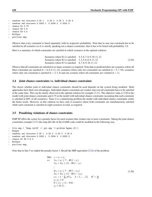
630 Stochastic Programming (SP) with EMP 3 randvar om1 discrete 0.25 1 0.25 2 0.25 3 0.25 4 4 randvar om2 discrete 0.3333 1 0.3334 2 0.3333 3 5 chance E1 0.75 6 chance E2 0.6 7 chance E3 0.5 8 $offput 9 putclose emp; Observe that every constraint is listed separately with its respective probability. Note that in case one constraint has to be satisfied in all scenarios (so it is strictly speaking not a chance constraint), then it has to be listed with probability 1.0. Here is a summary of which constraints are satisfied in which scenarios in the optimal solution: Scenarios where E1 is satisfied: 4,5,6,7,8,9,10,11,12 Scenarios where E2 is satisfied: 2,3,5,6,8,9,11,12 Scenarios where E3 is satisfied: 6,7,8,9,10,11,12. Observe that all constraints are satisfied in as many scenarios as required. Note that as predicted there are scenarios where all three constraints are satisfied (k = 6,8,9,11,12), scenarios where only two constraints are satisfied (k = 5,7,10), scenarios where only one constraint is satisfied (k = 2,3,4) and one scenario where all constraints are violated (k = 1). 3.4 Joint chance constraints vs. individual chance constraints The choice whether joint or individual chance constraints should be used depends on the system being modeled. Both approaches have their own advantages. Individual chance constraints are weaker since not all constraints have to be satisfied at the same time. This can be clearly observed in the optimal solution for example (3.21). The objective value is 5.20 in the model with joint chance constraints and 4.75 in the model with individual chance constraints (assuming that each constraint is satisfied in 60% of all scenarios). Since it is a minimizing problem the model with individual chance constraints yields the better result. However, in this solution we have only 6 scenarios where both constraints are simultaneously satisfied while each constraint is satisfied in eight scenarios in total, as required. 3.5 Penalizing violations of chance constraints EMP SP offers the syntax for a penalty factor for each scenario that violates one or more constraints. Taking the joint chance constraints example (3.21) the emp.info file of the GAMS code could be modified in the following way: 1 file emp / ’%emp.info%’ /; put emp ’* problem %gams.i%’/; 2 $onput 3 randvar om1 discrete 0.25 1 0.25 2 0.25 3 0.25 4 4 randvar om2 discrete 0.3333 1 0.3334 2 0.3333 3 5 chance E1 E2 0.6 3 6 $offput 7 putclose emp; Note that in line 5 we added the penalty factor 3. Recall the MIP equivalent (3.24) of the problem: Min z = x1 + x2 s.t. 1x1 + x2 ≥ 7 − M(1 − y1) 1x1 + 3x2 ≥ 12 − M(1 − y1) . 4x1 + x2 ≥ 7 − M(1 − y12) 3x1 + 3x2 ≥ 12 − M(1 − y12) cc1 = 1 − ∑k π k yk, k = 1,...,12, π k = 1 12 x1,x2 ≥ 0 0 ≤ cc1 ≤ (1 − 0.6) yk ∈ (0,1). (3.29) (3.30)
Stochastic Programming (SP) with EMP 631 The probability with which the constraints were violated is stored in the variable cc1 . The introduction of the penalty factor on line 5 of the emp.info file causes cc1 multiplied by the penalty factor to be added to the objective function: Similarly, the lines chance E1 0.75 5 chance E2 0.6 6 chance E3 0.5 7 z = x1 + x2 + 3cc1. (3.31) in the emp.info file of the GAMS code for the problem with individual chance constraints (3.25) trigger the objective function in the MIP equivalent to become: This can be useful in order to explore sensitivities to slight changes. z = x1 + x2 + 5cc1 + 6cc2 + 7cc3. (3.32) There is also a possibility that allows the modeler to use the probability expression as a variable in the original model. For example, in the joint chance constraints problem above we could introduce a new variable, viol, in the objective function: Then we replace line 5 in the emp.info file of the GAMS code as follows: chance E1 E2 0.6 viol This addition causes cc1 to be replaced by viol in the MIP equivalent. Thus we have: viol = 1 −∑ k Min z = x1 + x2 + 3 ∗ viol (3.33) π k yk, k = 1,...,12, π k = 1 , viol ∈ [0,0.4]. (3.34) 12 This model is equivalent to the joint chance constraints model with penalty factor 3 with which we started this section. 4 Risk Measures Risk measures are mechanisms to evaluate the effects of uncertainty in the underlying system on the outcomes of interest. They can be used to modify the distribution of outcomes. In this section we explore how optimization problems involving risk measures can be modeled using stochastic programming in GAMS EMP. Specifically, we examine how an investor might seek to balance expected rewards and the risk of loss when she decides how to allocate assets in a portfolio. First, we will discuss maximizing the expected value of a portfolio with uncertain returns, then we will briefly introduce the notion of Value at Risk and finally we will examine optimization problems involving Conditional Value at Risk and a combination of expected value and Conditional Value at Risk. For simplicity we consider only one period of uncertainty (0,T ) between the two dates 0 and T . In the examples introduced below the period (0,T ) is the period between investing in a portfolio of assets and return from this portfolio. 4.1 Expected Value Suppose an investor has the opportunity to invest a certain amount in three assets. She is given the probability distribution in Table 29.3 that links each asset with a possible return at time T . The question arises how she should allocate her funds between the three assets at time 0 in order to maximise her expected return at time T.
Page 1 and 2: Stochastic Programming (SP) with EM
Page 13: Stochastic Programming (SP) with EM
Page 21 and 22: 6 Stochastic Programming (SP) with

Stochastic Programming (SP) with EMP - Gams

Create successful ePaper yourself

Delete template?

Save as template?