

Stochastic Programming (SP) with EMP - Gams
Stochastic Programming (SP) with EMP - Gams
Stochastic Programming (SP) with EMP - Gams

You also want an ePaper? Increase the reach of your titles
YUMPU automatically turns print PDFs into web optimized ePapers that Google loves.
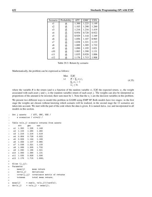
632 <strong>Stochastic</strong> <strong>Programming</strong> (<strong>SP</strong>) <strong>with</strong> <strong>EMP</strong><br />
Mathematically, the problem can be expressed as follows:<br />
Scenario Probability ATT GMC USX<br />
s1 1 12 1.300 1.225 1.149<br />
s2 1 12 1.103 1.290 1.260<br />
s3 1 12 1.216 1.216 1.419<br />
s4 1 12 0.954 0.728 0.922<br />
s5 1 12 0.929 1.144 1.169<br />
s6 1 12 1.056 1.107 0.965<br />
s7 1 12 1.038 1.321 1.133<br />
s8 1 12 1.089 1.305 1.732<br />
s9 1 12 1.090 1.195 1.021<br />
s10 1 12 1.083 1.390 1.131<br />
s11 1 12 1.035 0.928 1.006<br />
s12 1 12 1.176 1.715 1.908<br />
Table 29.3: Return by scenario<br />
Max E[R]<br />
s.t R = ∑ j w jv j<br />
∑ j w j = 1<br />
w j ≥ 0,<br />
where the variable R is the return (and is a function of the random variable v), E[R] the expected return, w j the weight<br />
associated <strong>with</strong> each asset j and v j is the (random variable) return of each asset j. The weights can also be interpreted as<br />
proportions of the amount to be invested, their sum must be 1. Note that the w j’s are the decision variables in this problem.<br />
We present two different ways to model this problem in GAMS using <strong>EMP</strong> <strong>SP</strong>. Both models have two stages: in the first<br />
stage the weights are chosen <strong>with</strong>out knowing which scenario will be realized, in the second stage the 12 scenarios are<br />
taken into account. We start <strong>with</strong> the part of the code where the data is given. It is named data.inc and incorporated in all<br />
models in this section.<br />
1 Set j assets / ATT, GMC, USX /<br />
2 s scenarios / s1*s12 /<br />
3<br />
4 Table vs(s,j) scenario returns from assets<br />
5 att gmc usx<br />
6 s1 1.300 1.225 1.149<br />
7 s2 1.103 1.290 1.260<br />
8 s3 1.216 1.216 1.419<br />
9 s4 0.954 0.728 0.922<br />
10 s5 0.929 1.144 1.169<br />
11 s6 1.056 1.107 0.965<br />
12 s7 1.038 1.321 1.133<br />
13 s8 1.089 1.305 1.732<br />
14 s9 1.090 1.195 1.021<br />
15 s10 1.083 1.390 1.131<br />
16 s11 1.035 0.928 1.006<br />
17 s12 1.176 1.715 1.908;<br />
18<br />
19 Alias (j,jj);<br />
20 Parameter<br />
21 mean(j) mean return<br />
22 dev(s,j) deviations<br />
23 covar(j,jj) covariance matrix of returns<br />
24 totmean total mean return;<br />
25<br />
26 mean(j) = sum(s, vs(s,j))/card(s);<br />
27 dev(s,j) = vs(s,j) - mean(j);<br />
(4.35)


