Solutions chapter 4 - Cosmology and particle astrophysics

Solutions chapter 4 - Cosmology and particle astrophysics
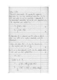
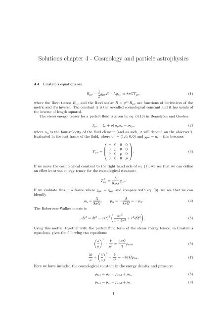
4.4 Einstein’s equations are
Rµν − 1
2 gµνR − Λgµν = 8πGTµν, (1)
where the Ricci tensor Rµν and the Ricci scalar R = g µν Rµν are functions of derivatives of the
metric and it’s inverse. The constant Λ is the so-called cosmological constant and it has usints of
the inverse of length squared.
The stress energy tensor for a perfect fluid is given by eq. (4.13) in Bergström and Goobar:
Tµν = (p + ρ) uµuν − pgµν
where uµ is the four-velocity of the fluid element (and as such, it will depend on the observer!).
Evaluated in the rest frame of the fluid, where u µ = (1, 0, 0, 0) and gµν = ηµν, this becomes
⎛
ρ
⎜
Tµν = ⎜ 0
⎝ 0
0
p
0
0
0
p
0
0
0
⎞
⎟
⎠ . (3)
0 0 0 p
If we move the cosmological constant to the right hand side of eq. (1), we see that we can define
an effective stress energy tensor for the cosmological constant:
T Λ µν = Λ
8πG gµν.
If we evaluate this in a frame where gµν = ηµν and compare with eq. (3), we see that we can
identify
ρΛ = Λ
8πG , pΛ = − Λ
8πG = −ρΛ. (4)
The Robertson-Walker metric is
ds 2 = dt 2 − a (t) 2
dr 2
1 − kr 2 + r2 dΩ 2
(2)
. (5)
Using this metric, together with the perfect fluid form of the stress energy tensor, in Einstein’s
equations, gives the following two equations:
2ä
a +
2 ˙a
a
+ k 8πG
=
a2 3 ρtot, (6)
2 ˙a
+
a
k
a2 = −8πGptot. (7)
Here we have included the cosmological constant in the energy density and pressure:
ρtot = ρm + ρrad + ρΛ, (8)
ptot = pm + prad + pΛ. (9)
1

Eq. (6) is the 00-component of Einstein’s equations, where as the second equation comes from
the spatial component.
independent equation.
Notice that by isotropy, the spatial component can only give us one
By construction, the left hand side of Einstein’s equation has a vanishing divergence:
Rµν − 1
2 gµνR
− Λgµν = 0. (10)
This means that the right hand side must also have vanishing divergence:
;ν
T µν ;ν = 0. (11)
Using the Robertson-Walker metric and the perfect fluid form of the stress energy tensor then
gives
˙ρ + 3H (ρ + p) = 0, (12)
which has the physically meaning of: “a change in the energy density equals the flow of energy
density into that region.” Notice that we need to include pressure here, since pressure is a form of
energy. The factor 3H appears in a lot of places in cosmology, and it can be viewed as a measure
of how much a three-volume changes due to the expansion of space.
Before we start to manipulate Einstein’s equation, we try to solve eq. (12). Introducing an
equation of state
p = wρ (13)
casts the continuity equation in the form
or
which can be solved to give
˙ρ + 3H (1 + w) ρ = 0 (14)
dρ 1
dt ρ
da 1
= −3 (1 + w)
dt a
ρ ∼ a −3(1+w)
where the proportionality constant depends on how large the energy density is at a given some
given time.
If we now take the difference between the two Einstein equations, we get
(15)
(16)
ä
= −4πG (ρ + 3p) . (17)
a 3
Notice how the curvature term ka −2 dropped out. This means that we can solve for the evolution
of a as a function of the energy density and pressure (which are related by the equation of
state), and then set initial conditions according to the 00-equation (which includes the curvature).
Using eq. (16) and the equation of state in eq. (13) turns the left hand side into (we now use a
proportionality constant in the equations)
or
Using the ansatz a (t) ∼ t β then gives
or
ä
∼ a−3(1+w)
a
(18)
ä ∼ a −2−3w . (19)
t β−2 ∼ t −(2+3w)β , (20)
β =
2
3 (1 + w)
2
(21)

so
2
a (t) ∼ t 3(1+w) . (22)
Notice that if w = −1 we would not be able to determine β, which tells us that our ansatz was
not good. Instead, we would get the equation
with solution
ä ∼ a (23)
a ∼ exp (±At) , (24)
for some constant A with units of s −1 (which from the Friedmann equation can be determined to
be equal to
Λ
3 ).
4.7 The Hubble function is given from Einstein’s equation as
H (t) 2 ≡
2 ˙a
=
a
8πG
3 (ρm + ρvac) − k
a2 = 8πG
3 ρm + Λ k
− . (25)
3 a2 We know that the matter scales as the inverse cube of the scale factor, so we can write
ρm = ρ0a3 0
3 , (26)
a (t)
where a0 is the scale factor today and ρ0 is the matter density today. If we now define
ΩM ≡ 8πGρ0
3H2 , ΩΛ ≡
0
Λ
3H2 , ΩK ≡
0
−k
a2 0H2 , (27)
0
where H 2 0 is the value of the Hubble function today, we can write the Hubble function as
For the redshift we have that
H (t) 2 = H 2 0
= H 2 0
= H 2 0
8πG
3H 2 0
ΩM
8πG
ρ0a 3 0
a (t)
3H 2 0
a 3 0
ρm + Λ
3H 2 0
3H 2 0
3 + Λ
− k
H 2 0 a2 0
− k
H 2 0 a2
a 2 0
a (t) 3 + ΩΛ + ΩK
a (t) 2
a 2 0
a (t) 2
. (28)
a0
= 1 + z, (29)
a (t)
which means that we can finally write the Hubble function as
ΩM (1 + z) 3 + ΩΛ + ΩK (1 + z) 2
. (30)
H (t) 2 = H 2 0
Notice that we have neglected the contribution from radiation, which should be perfectly fine for
z < 1000.
3

4.11 We assume a “standard” cosmology with
Volumes in the universe will change as
ΩM + ΩR = 1, ΩΛ = 0, (31)
H0 = 65 km s −1 Mpc −1 . (32)
V (t) = V0
a (t)
a0
3
, (33)
where V0 is the given volume today and a0 is the scale factor today. The Hubble function is
H 2 = H 2 0
= H 2 0
ΩM
ΩM (1 + z) 3 + ΩR (1 + z) 4
For an order of magnitude estimate, we can drop ΩR. Using H = ˙a
a
or
3
3
a0
a0
+ ΩR . (34)
a (t) a (t)
˙a 2 = H2 0 ΩM a 3 0
a (t)
da
dt
we get
(35)
∼ 1
√ a . (36)
Notice that we drop the numerical factor here: It doesn’t matter since we only need to compute
the relative change in the scale factor. The above differential equation can be solved to give
or
We thus get
a (t) ∼ t 2/3
a (t) = a0
V (t) = V0
t
t0
t
(37)
2/3
. (38)
t0
2
. (39)
We now need to determine V0 and t0. The age of the universe is given by integrating equation
(4.77):
t0 = H −1
ˆ∞
dz 2
0
= . (40)
5/2
(1 + z) 3H0
0
The volume of the observable universe is given by the particle horizon, which tells us how far a
photon can have travelled since t = 0. It is given by equation (4.89):
ˆ
dH (t) = a (t)
Since we want to study this for t = t0 this becomes
dH (t0) = a0
ˆt0
0
a0
t ′
t0
0
t
dt ′
a (t ′ . (41)
)
dt ′
= 3t0 =
2/3 2
. (42)
4
H0

The volume is then V0 ∼ [dH (t0)] 3 ∼ t 3 0 (notice that we are using a order of magnitude estimate,
since we have neglected the contribuation from ΩR anyways) and we thus get
V (t) ∼ t0t 2 ∼ t2
To get the right unit we must also put in a factor of c 3 here:
V (t) ∼ c3 t 2
Now comes the difficult part: Plugging in actual numbers. We have
This gives
H0
H0
. (43)
. (44)
c = 3 × 10 8 m s −1 , H0 = 2 × 10 −18 s −1 , t = 10 −3 s. (45)
V t = 10 −3 s ∼ 10 37 m 3 . (46)
We can compare this to our estimate of the observable universe today, which is
4.13 We have the relation
V0 ∼ c 3 t 3 0 ∼ 10 78 m 3 . (47)
m (z) = M + 5 log 10 dL (z) + 25 (48)
where m is the apparent magnitude, M the absolute magnitude (the apparent magnitude if the
object is at 10 parsec from the observer) and dL is measured in Mpc. Solving for dL gives
For our values we have
which gives
dL = 10 m−M−25
5 Mpc. (49)
m = 18, M = −17, (50)
dL = 10 18+17−25
2 Mpc = 100 Mpc. (51)
5