OQNLP and MSNLP - Gams

OQNLP and MSNLP
Optimal Methods Inc, 7134 Valburn Dr., Austin, TX 78731 www.optimalmethods.com, 512-346-7837
OptTek System, Inc., 1919 7th St., Boulder, CO 80302, www.opttek.com, 303-447-3255
Contents
1 Introduction . . . . . . . . . . . . . . . . . . . . . . . . . . . . . . . . . . . . . . . . . . . . . . . . . . 369
2 Combining Search Methods and Gradient-Based NLP Solvers . . . . . . . . . . . . . . . . . . . . . . 371
3 Output . . . . . . . . . . . . . . . . . . . . . . . . . . . . . . . . . . . . . . . . . . . . . . . . . . . . . 371
3.1 Log File . . . . . . . . . . . . . . . . . . . . . . . . . . . . . . . . . . . . . . . . . . . . . . . . . 371
3.2 The LOCALS File . . . . . . . . . . . . . . . . . . . . . . . . . . . . . . . . . . . . . . . . . . . 373
4 The Options File . . . . . . . . . . . . . . . . . . . . . . . . . . . . . . . . . . . . . . . . . . . . . . . . 373
5 Use as a Callable System . . . . . . . . . . . . . . . . . . . . . . . . . . . . . . . . . . . . . . . . . . . 377
Appendix A: Description of the Algorithm . . . . . . . . . . . . . . . . . . . . . . . . . . . . . . . . . . . . 377
Appendix B: Pure and ”Smart” Random Drivers . . . . . . . . . . . . . . . . . . . . . . . . . . . . . . . . . 379
References . . . . . . . . . . . . . . . . . . . . . . . . . . . . . . . . . . . . . . . . . . . . . . . . . . . . . . 380
1 Introduction
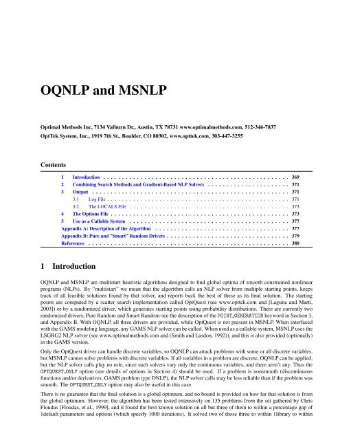
OQNLP and MSNLP are multistart heuristic algorithms designed to find global optima of smooth constrained nonlinear
programs (NLPs). By ”multistart” we mean that the algorithm calls an NLP solver from multiple starting points, keeps
track of all feasible solutions found by that solver, and reports back the best of these as its final solution. The starting
points are computed by a scatter search implementation called OptQuest (see www.opttek.com and [Laguna and Marti,
2003]) or by a randomized driver, which generates starting points using probability distributions. There are currently two
randomized drivers, Pure Random and Smart Random-see the description of the POINT GENERATION keyword in Section 3,
and Appendix B. With OQNLP, all three drivers are provided, while OptQuest is not present in MSNLP. When interfaced
with the GAMS modeling language, any GAMS NLP solver can be called. When used as a callable system, MSNLP uses the
LSGRG2 NLP solver (see www.optimalmethods.com and (Smith and Lasdon, 1992)), and this is also provided (optionally)
in the GAMS version.
Only the OptQuest driver can handle discrete variables, so OQNLP can attack problems with some or all discrete variables,
but MSNLP cannot solve problems with discrete variables. If all variables in a problem are discrete, OQNLP can be applied,
but the NLP solver calls play no role, since such solvers vary only the continuous variables, and there aren’t any. Thus the
OPTQUEST ONLY option (see details of options in Section 4) should be used. If a problem is nonsmooth (discontinuous
functions and/or derivatives, GAMS problem type DNLP), the NLP solver calls may be less reliable than if the problem was
smooth. The OPTQUEST ONLY option may also be useful in this case.
There is no guarantee that the final solution is a global optimum, and no bound is provided on how far that solution is from
the global optimum. However, the algorithm has been tested extensively on 135 problems from the set gathered by Chris
Floudas [Floudas, et al., 1999], and it found the best known solution on all but three of them to within a percentage gap of
1default parameters and options (which specify 1000 iterations). It solved two of those three to within 1library to within

370 OQNLP and MSNLP
1seven remaining ones by increasing the iteration limit or using another NLP solver. These results are described in [Lasdon
et al., 2004]. For more information on OQNLP, see [Ugray, et. al., 2003].
A multistart algorithm can improve the reliability of any NLP solver, by calling it with many starting points. If you have a
problem where you think the current NLP solver is failing to find even a local solution, choose an NLP solver and a limit
on the number of solver calls, and try OQNLP or MSNLP. Even if a single call to the solver fails, multiple calls from the
widely spaced starting points provided by this algorithm have a much better chance of success.
Often an NLP solver fails when it terminates at an infeasible solution. In this situation, the user is not sure if the problem
is really infeasible or if the solver is at fault (if all constraints are linear or convex the problem is most likely infeasible). A
multistart algorithm can help in such cases. To use it, the problem can be solved in its original form, and some solver calls
may terminate with feasible solutions. The algorithm will return the best of these. If all solver calls terminate infeasible,
the problem can be reformulated as a feasibility problem. That is, introduce ”deviation” or ”elastic” variables into each
constraint, which measure the amount by which it is violated, and minimize the sum of these violations, ignoring the true
objective. OQNLP or MSNLP can be applied to this problem, and either has a much better chance of finding a feasible
solution (if one exists) than does a single call to an NLP solver. If no feasible solution is found, you have much more
confidence that the problem is truly infeasible.
The OptQuest and randomized drivers generate trial points which are candidate starting points for the NLP solver. These
are filtered to provide a smaller subset from which the solver attempts to find a local optimum. In the discussion which
follows, we refer to this NLP solver as ”L.”, for Local solver.
The most general problem OQNLP can solve has the form
subject to the nonlinear constraints
and the linear constraints
minimize f (x,y) (1.1)
gl ≤ G(x,y) ≤ gu (1.2)
l ≤ A1x + A2y ≤ u (1.3)
x ∈ S, y ∈ Y (1.4)
where x is an n-dimensional vector of continuous decision variables, y is a p-dimensional vector of discrete decision variables,
and the vectors gl,gu,l, and u contain upper and lower bounds for the nonlinear and linear constraints respectively.
The matrices A1 and A2 are m2 by n and m2 by p respectively, and contain the coefficients of any linear constraints. The set
S is defined by simple bounds on x, and we assume that it is closed and bounded, i.e., that each component of x has a finite
upper and lower bound. This is required by all drivers (see section 4 for a discussion of the parameter ARTIFICIAL BOUND
which provides bounds when none are specified in the model). The set Y is assumed to be finite, and is often the set of all
p-dimensional binary or integer vectors y. The objective function f and the m1- dimensional vector of constraint functions
G are assumed to have continuous first partial derivatives at all points in S ×Y . This is necessary so that L can be applied
to the relaxed NLP sub-problems formed from 1.1 - 1.4 by allowing the y variables to be continuous. The MSNLP system
does not allow any discrete variables.
An important function used in this multistart algorithm is the L1 exact penalty function, defined as
P1(x,w) = f (x) +
m
∑
i=1
Wiviol(gi(x)) (1.5)
where the wi are nonnegative penalty weights, m = m1 + m2, and the vector g has been extended to include the linear
constraints 1.4. For simplicity, we assume there are no y variables: these would be fixed when this function is used. The
function viol(gi(x)) is equal to the absolute amount by which the ith constraint is violated at the point x. It is well known
(see [Nash and Sofer, 1996]) that if x ∗ is a local optimum of 1.1 - 1.4, u ∗ is a corresponding optimal multiplier vector, the
second order sufficiency conditions are satisfied at (x ∗ ,u ∗ ) , and
wt > abs(u ∗ i ) (1.6)
then x ∗ is a local unconstrained minimum of P1 . If 1.1 - 1.4 has several local minima, and each wi

OQNLP and MSNLP 371
is larger than the maximum of all absolute multipliers for constraint i over all these optima, then Pi has a local minimum at
each of these local constrained minima. We will use Pi to set thresholds in the merit filter.
2 Combining Search Methods and Gradient-Based NLP Solvers
For smooth problems, the relative advantages of a search method over a gradient-based NLP solver are its ability to locate
an approximation to a good local solution (often the global optimum), and the fact that it can handle discrete variables.
Gradient-based NLP solvers converge to the ”nearest” local solution, and have no facilities for discrete variables, unless
they are imbedded in a rounding heuristic or branch-and-bound method. Relative disadvantages of search methods are their
limited accuracy, and their weak abilities to deal with equality constraints (more generally, narrow feasible regions). They
find it difficult to satisfy many nonlinear constraints to high accuracy, but this is a strength of gradient-based NLP solvers.
Search methods also require an excessive number of iterations to find approximations to local or global optima accurate to
more than two or three significant figures, while gradient-based solvers usually achieve four to eight-digit accuracy rapidly.
The motivation for combining search and gradient- based solvers in a multi-start procedure is to achieve the advantages of
both while avoiding the disadvantages of either.
3 Output
3.1 Log File
When it operates as a GAMS solver, OQNLP and MSNLP will by default write information on their progress to the GAMS
log file. When used as a callable system, this information, if requested, will be written to a file opened in the users calling
program. The information written consists of:
1. Echos of important configuration and setup values
2. Echo (optionally) of options file settings processed
3. Echos of important algorithm settings, parameters, and termination criteria
4. The iteration log
5. Final results, termination messages, and status report
A segment of that iteration log from stages 1 and 2 of the algorithm is shown below for the problem ex8 6 2 30.gms, which
is one of a large set of problems described in [Floudas, et al., 1999]. This is a 91 variable unconstrained minimization
problem, available from GLOBALLib at www.gamsworld.org/global. There are 200 iterations in stage one and 1000
total iterations (see Appendix A for an algorithm description), with output every 20 iterations and every solver call.
The headings below have the following meanings:
Itn iteration number
Penval Penalty function value
Merit Filter ACC if the merit filter accepts the point, REJ if it rejects
Merit
threshold value for merit filter: accepts if Penval < Threshold
Threshold
Dist Filter ACC if the distance filter accepts the point, REJ if it rejects
Best Obj Best feasible objective value found thus far
Solver Obj Objective value found by NLP solver at this iteration
Term Code Code indicating reason for termination of NLP solver:
KTC means Kuhn-Tucker optimality conditions satisfied
FRC means that the fractional objective change is less than a tolerance for some number of consecutive
iterations
INF means solver stopped at an infeasible point
Sinf sum of infeasibilities at point found by NLP solver

372 OQNLP and MSNLP
Iterations 0 through 200 below show the initial NLP solver call (at the user-specified initial point, which finds a local
minimum with objective value -161.8), and every 20th iteration of stage 1, which has no other solver calls. At iteration 200
stage 1 ends, and th solver is started at the best of the 200 stage 1 points, finding a local min with objective -176.0. The
next solver call at iteration 207 finds a better objective of -176.4. Note that, at iteration 207, the OptQuest trial solution has
a Penval of -23.18, and this is less than the merit threshold of -20.75, so the merit filter ACCepts the trial solution, as does
the distance filter. The next 9 solver calls fail to improve this value, so Best Obj remains the same, until at iteration 432
a solution with value -176.6 is found. At iteration 473, the solver call finds a value of -177.5. Further solver calls do not
find an improved solution and are not shown. The solution with value -177.5 is the best known solution, but OQNLP cannot
guarantee this.
Itn Penval Merit Merit Dist Best Solver Term Sinf
Filter Threshold Filter Obj Obj Code
0 +1.000e+030 -1.000e+030 -1.618e+002 -1.618e+002 FRC +0.000e+000
20 -4.485e+000
40 -6.321e+000
60 -1.126e+001
80 +2.454e+000
100 +8.097e+001
120 +5.587e+001
140 +1.707e+004
160 +2.034e+002
180 +7.754e+001
200 -6.224e+000
Itn Penval Merit Merit Dist Best Solver Term Sinf
Filter Threshold Filter Obj Obj Code
201 +1.000e+030 ACC -1.000e+030 ACC -1.618e+002 -1.760e+002 FRC +0.000e+000
207 -2.318e+001 ACC -2.075e+001 ACC -1.760e+002 -1.764e+002 FRC +0.000e+000
220 -8.324e+000 REJ -2.318e+001 ACC -1.764e+002
240 +8.351e+000 REJ -1.834e+001 ACC -1.764e+002
251 -1.117e+001 ACC -1.008e+001 ACC -1.764e+002 -1.682e+002 FRC +0.000e+000
256 -1.244e+001 ACC -1.117e+001 ACC -1.764e+002 -1.758e+002 FRC +0.000e+000
258 -1.550e+001 ACC -1.244e+001 ACC -1.764e+002 -1.678e+002 FRC +0.000e+000
260 -7.255e+000 REJ -1.550e+001 ACC -1.764e+002
280 +8.170e+001 REJ -1.220e+001 ACC -1.764e+002
282 -2.521e+001 ACC -1.220e+001 ACC -1.764e+002 -1.758e+002 FRC +0.000e+000
300 +5.206e+001 REJ -2.521e+001 ACC -1.764e+002
300 +5.206e+001 REJ -2.521e+001 ACC -1.764e+002
320 +1.152e+000 REJ -1.642e+001 ACC -1.764e+002
329 -2.111e+001 ACC -1.294e+001 ACC -1.764e+002 -1.763e+002 FRC +0.000e+000
338 -3.749e+001 ACC -2.111e+001 ACC -1.764e+002 -1.763e+002 FRC +0.000e+000
340 +2.235e+002 REJ -3.749e+001 ACC -1.764e+002
360 +8.947e+001 REJ -2.363e+001 ACC -1.764e+002
366 -3.742e+001 ACC -2.363e+001 ACC -1.764e+002 -1.761e+002 FRC +0.000e+000
380 -2.244e+001 REJ -3.742e+001 ACC -1.764e+002
391 -2.974e+001 ACC -2.244e+001 ACC -1.764e+002 -1.754e+002 FRC +0.000e+000
400 +1.986e+002 REJ -2.974e+001 ACC -1.764e+002
400 +1.986e+002 REJ -2.974e+001 ACC -1.764e+002
420 -1.231e+001 REJ -2.359e+001 ACC -1.764e+002
432 -2.365e+001 ACC -2.359e+001 ACC -1.764e+002 -1.766e+002 FRC +0.000e+000
440 +6.335e+000 REJ -2.365e+001 ACC -1.766e+002
460 -8.939e+000 REJ -1.872e+001 ACC -1.766e+002
473 -3.216e+001 ACC -1.872e+001 ACC -1.766e+002 -1.775e+002 FRC +0.000e+000
480 +1.744e+002 REJ -3.216e+001 ACC -1.775e+002

OQNLP and MSNLP 373
3.2 The LOCALS File
The LOCALS file is a text file containing objective and variable values for all local solutions found by MSNLP. It is
controlled by the LOCALS FILE and LOCALS FILE FORMAT keywords in the MSNLP Options file. An example for the
problem EX 8 1 5 from the Floudas problem set (available on www.gamsworld.org, link to globalworld) is shown below.
The headings, included for explanatory purposes and not part of the file, have the following meaning:
No. index of local solution
Obj objective value of local solution
Var variable index
Value variable value
No. Obj Var Value
1 -1.03163e+000 1 -8.98448e-002
1 -1.03163e+000 2 7.12656e-001
2 -1.03163e+000 1 8.98418e-002
2 -1.03163e+000 2 -7.12656e-001
3 -2.15464e-001 1 1.70361e+000
3 -2.15464e-001 2 -7.96084e-001
4 -2.15464e-001 1 -1.70361e+000
4 -2.15464e-001 2 7.96084e-001
5 0.00000e+000 1 0.00000e+000
5 0.00000e+000 2 0.00000e+000
6 2.10425e+000 1 1.60710e+000
6 2.10425e+000 2 5.68656e-001
7 2.10425e+000 1 -1.60711e+000
7 2.10425e+000 2 -5.68651e-001
Thus local solutions 1 and 2 both have objective values of -1.03163. The first solution has variable values x = -8.98448e-
002, y = 7.12656e-001, where these are in the same order as they are defined in the gams model. The second local solution
has x = 8.98418e-002, y = -7.12656e-001. Seven local solutions are found. This output is produced with all default
parameter values for MSNLP options and tolerances, except the distance and merit filters were turned off, i.e the keywords
USE DISTANCE FILTER and USE MERIT FILTER were set to 0 in the MSNLP options file. This causes the NLP solver to
be called at every stage 2 trial point, and is recommended if you wish to obtain as many local solutions as possible.
4 The Options File
The options file is a text file containing a set of records, one per line. Each record has the form ,
where the keyword and value are separated by one or more spaces. All relevant options are listed in this guide. You can also
get a sample option file with all options and their default values by specifying the single option help in an option file. The
list of all options appears in the log file. The options are described below.

374 OQNLP and MSNLP
Option Description Default
ARTIFICIAL BOUND This value (its negative) is given to the driver as the upper (lower) bound for
any variable with no upper or lower bound. However, the original bounds are
given to the local solver, so it can produce solutions not limited by this artificial
bound. All drivers must have finite upper and lower bounds for each variable.
If ARTIFICIAL BOUND (or any of the user- supplied bounds) is much larger than
any component of the optimal solution, the driver will be less efficient because
it is searching over a region that is much larger than needed. Hence the user is
advised to try to provide realistic values for all upper and lower bounds. It is
even more dangerous to make ARTIFICIAL BOUND smaller than some component
of a globally optimal solution, since the driver can never generate a trial
point near that solution. It is possible, however, for the local solver to reach a
global solution in this case, since the artificial bounds are not imposed on it.
1.e4
BASIN DECREASE This value must be between 0 and 1. If DYNAMIC DISTANCE FILTER is set 0.2
FACTOR
to 1, the MAXDIST value associated with any local solution is reduced by
(1-BASIN DECREASE FACTOR) if WAITCYCLE consecutive trial points have distance
from that solution less than MAXDIST.
BASIN OVERLAP FIX A value of 1 turns on logic which checks the MAXDIST values of all pairs of local
solutions, and reduces any pair of MAXDIST values if their sum is greater than the
distance between the 2 solutions. This ensures that the spherical models of their
basins of attracting do not overlap. A value of 0 turns off this logic. Turning it
off can reduce the number of NLP solver calls, but can also cause the algorithm
to miss the global solution.
1
DISTANCE FACTOR If the distance between a trial point and any local solution found previously is
less than DISTANCE FACTOR ∗ MAXDIST, the NLP solver is not started from that
trial point. MAXDIST is the largest distance ever traveled to get to that local
solution. Increasing DISTANCE FACTOR leads to fewer solver calls and risks
finding a worse solution. Decreasing it leads to more solver calls and possibly a
better solution.
1.0
DYNAMIC DISTANCE A value of 1 turns on logic which reduces the value of MAXDIST (described under 1
FILTER
the USE DISTANCE FILTER keyword) for a local solution if WAITCYCLE consecutive
trial points have a their distances from that solution less than MAXDIST.
MAXDIST is multiplied by (1-BASIN REDUCTION FACTOR). A value of 0 turns
off this logic. Turning it off can decrease the number of NLP solver calls, but
can also lead to a worse final solution.
DYNAMIC MERIT FILTER A value of 1 turns on logic which dynamically varies the parameter which increases
the merit filter threshold, THRESHOLD INCREASE FACTOR. If WAITCYCLE
consecutive trial points have been rejected by the merit filter, this value is replaced
by max(THRESHOLD INCREASE FACTOR, val), where val is the value of
THRESHOLD INCREASE FACTOR which causes the merit filter to just accept the
best of the previous WAITCYCLE trial points. A value of 0 turns off this logic.
Turning it off can reduce NLP solver calls, but may lead to a worse final solution.
1
ENABLE SCREEN OUTPUT A value of 0 turns off the writing of the iteration log and termination messages
to the gams log file that appears on the screen, while 1 enables it.
1
ENABLE STATISTICS Using a value of 1 creates a text file called stats.log in the project directory 0
LOG
containing one line of problem (name, variables, constraints) and performance
information (best objective value, total solver time, iterations, iterations to best
solution, etc) for each problem solved.

OQNLP and MSNLP 375
Option Description Default
FEASIBILITY This tolerance is used to check each point returned by an NLP solver for feasi- 1.e-4
TOLERANCE
bility. If the largest absolute infeasibility at the point is larger than this tolerance,
the point is classified infeasible. This test is made because points returned by
NLP solvers may occasionally be infeasible despite feasible status codes. Some
NLP solvers use internal scaling before testing for feasibility. The unscaled problem
may be infeasible, while the scaled one is feasible. If this occurs, increasing
this tolerance (to 1.e-2 or larger) often eliminates the problem.
ITERATION PRINT If the OQNLP iteration log is written to the GAMS log file, one line of output is 20
FREQUENCY
written every k’th OptQuest iteration, where k is the value given here.
ITERATION LIMIT Increasing this limit can allow OQNLP to find a better solution. Try it if your
run using 1000 iterations doesn’t take too long. Surprisingly, the best solution
using, say 2000 iterations, may be found in the first 1000 iterations, and that
solution may be better than the one found with an iteration limit of 1000. This
is because OptQuest changes its search strategy depending on the iteration limit.
Because of this, it is also possible that increasing the iteration limit will yield a
worse solution, but this is rare. Decreasing this iteration limit usually leads to a
worse solution, but also reduces run time. OQNLP iterations can not be set using
GAMS iterlim. The GAMS iterlim is used as the iteration limit for the NLP
subsolves in an OQNLP run
1000
LOCALS FILE Specify a complete path and name for a file to which the objective value and No lo-
values of all variables for all local solutions found will be written. For example, cals file
C:\mydirectory\locals.out. There are 2 possible formats for this file, specified
by the LOCALS FILE FORMAT option below. If there is no LOCALS FILE record
in the options file, the locals file will not be created.
created
LOCALS FILE FORMAT There are 2 possible values for this option. The REPORT entry creates the locals
file in a format designed to be examined easily by eye, but processed less easily
by a computer program or spreadsheet. The DATA1 entry creates a file with many
REPORT
records, each on a single line, each line having the following format:
of local optimum>

376 OQNLP and MSNLP
Option Description Default
OPTQUEST ONLY This option applies only to the OptQuest driver. If you think the NLP solver
is taking too long and/or not working well, choosing 1 will stop it from being
called. This may occur if the problem is of type ”DNLP”, where one or more
problem functions are discontinuous or have discontinuous derivatives. If the
problem has only discrete (integer) variables, choose 1, as there is nothing for
the NLP solver to do (since it optimizes over the continuous variables when the
integers are fixed, and there aren’t any).
0
OQNLP DEBUG Values of 1 or 2 cause more information to be written to the iteration log. The
default value of 0 suppresses all this output.
0
POINT GENERATION OPTQUEST causes trial points to be generated by the OptQuest driver
SMART-
RANDOM causes trial points to be generated by sampling each variable from a
uniform distribution defined within its bounds
SMARTRANDOM1 generates trial points by sampling each variable independently
from either normal or triangular distributions, whose parameters are determined
as described in Appendix A.
RANDOM1
(MSNLP)
OPTQUEST
(OQNLP)
SAMPLING
DISTRIBUTION
This keyword is relevant only when POINT GENERATION is set to
SMARTRANDOM1. Then a value of 0 causes normal distributions to be used
to generate trial points, while a value of 1 causes triangular distributions to be
used.
SEARCH TYPE This option applies only to the OptQuest driver, and controls the search strategy
used by OptQuest. The three choices that are relevant for use within OQNLP
are:
aggressive This choice controls the population update in step 7 of the OptQuest
algorithm (see Appendix A). It triggers a very aggressive update,
which keeps the best of the points generated from the current population
as the new population. The risk in this is that all points in the new population
may cluster in a small portion of the search volume, and regions far
from this volume will not be explored in the next cycle.
boundary This option affects the trial points generated by OptQuest, directing
them toward the boundary of the region defined by the linear constraints
and variable bounds. The value of SEARCH PARAMETER discussed below
controls the fraction of points that are directed toward the boundary.
crossover This option affects how OptQuest trial points are generated from
population points. It retains the linear combination operator discussed
in Appendix A, but adds a ”crossover” operator, similar to those used in
evolutionary or genetic algorithms, to create 2 additional trial points.
SOLVELINK This option defines the solvelink used for the NLP solver:
1: Call NLP solver via script
2: Call NLP and MIP solver via module
5: Call NLP and MIP solver in memory
SOLVER LOG TO GAMS
LOG
Setting the parameter to 1 instructs OQNLP to copy the log from the NLP subsolver
to the OQNLP log. It can be very helpful to inspect the NLP subsolver
log especially if the solver termination code is ”???”.
STAGE1 ITERATIONS Specifies the total number of iterations in stage 1 of the algorithm, where no
NLP solver calls are made. Increasing this sometimes leads to a better starting
point for the first local solver call in stage 2, at the cost of delaying that call.
THRESHOLD INCREASE
FACTOR
Decreasing it can lead to more solver calls, but the first call occurs sooner.
This value must be nonnegative. If there are WAITCYCLE (see below) consecutive
OptQuest iterations where the merit filter logic causes the NLP
solver not to be called, the merit threshold is increased by mutipling it by
(1+THRESHOLD INCREASE FACTOR)
0
boundary
5
0
200
0.2

OQNLP and MSNLP 377
Option Description Default
USE DISTANCE FILTER Use 0 to turn off the distance filter, the logic which starts the NLP solver at a
trial point only if the (Euclidean) distance from that point to any local solution
found thus far is greater than the distance threshold. Turning off the distance
filter leads to more solver calls and more run time, and increases the chances of
finding a global solution. Turn off both distance and merit filters to find (almost)
all local solutions.
1
USE LINEAR
This option applies only to the OptQuest driver, and to problems that have lin- 0
CONSTRAINTS ear constraints other than simple bounds on the variables. Using 1 (all OptQuest
trial points satisfy the linear constraints) often leads to fewer iterations and solver
calls, but OptQuest has to solve an LP to project each trial point onto the linear
constraints. For large problems (more than 100 variables), this can greatly increase
run time, so the default value is off (0).
USE MERIT FILTER Use 0 to turn off the merit filter, the logic which starts the NLP solver at a trial
point only if the penalty function value at that point is below the merit threshold.
This will lead to more solver calls, but increases the chances of finding a global
solution. Turn off both filters if you want to find (almost) all local solutions. This
will cause the solver to be called at each stage 2 iteration.
1
WAITCYCLE This value must be a positive integer. If the merit filter is used, and there 20
are WAITCYCLE consecutive iterations where the merit filter logic causes the
NLP solver not to be started, the merit filter threshold is increased by the factor
THRESHOLD INCREASE FACTOR (see above). Increasing WAITCYCLE usually
leads to fewer solver calls, but risks finding a worse solution. Decreasing it leads
to more solver calls, but may find a better solution.
5 Use as a Callable System
MSNLP and OQNLP is also available as a callable system. It currently uses the LSGRG2 NLP solver as its local solver,
but any other NLP solver could be included. A sample calling program is provided which a user can easily adapt. The
user must provide a C function which computes values of the objective and all constraint functions, given current values of
all variables. First partial derivatives of these functions can be approximated by forward or central differences, or may be
computed in a user-provided function.
Appendix A: Description of the Algorithm
A pseudo-code description of the MSNLP algorithm follows, in which SP(xt) denotes the starting point generator and xt is
the candidate starting point produced. We refer to the local NLP solver as L(xs,x f ), where xs is the starting point and x f
the final point. The function UPDATE LOCALS(xs,x f ,w) processes and stores solver output x f , using the starting point xs
to compute the distance from xs to x f , and produces updated penalty weights, w. For more details, see [Lasdon, Plummer
et al., 2004].
MSNLP Algorithm
STAGE 1
x0 = user initial point
Call L(x0,x f )
Call UPDATE LOCALS(x0,x f ,w)
FOR i = 1,n1 DO
Call SP(xt(i))
Evaluate P(xt(i),w)
ENDDO

378 OQNLP and MSNLP
xt ∗ = point yielding best value of P(xt(i),w) over all stage one points, (i = 1,2,...,n1).
call L(xt ∗ ,x f )
Call UPDATE LOCALS(xt ∗ ,x f ,w)
threshold = P(xt ∗ ,w)
STAGE 2
FOR i = 1,n2 DO
Call SP(xt(i))
Evaluate P(xt(i),w)
Perform merit and distance filter tests:
Call distance filter(xt(i), dstatus)
Call merit filter(xt(i), threshold, mstatus)
IF (dstatus and mstatus = ”accept”) THEN
Call L(xt(i),x f )
Call UPDATE LOCALS(xt(i),x f ,w)
ENDIF
ENDDO
After an initial call to L at the user-provided initial point, x0, stage 1 of the algorithm performs n1 iterations in which SP(xt)
is called, and the L1 exact penalty value P(xt,w) is calculated. The user can set n1 through the MSNLP options file using the
STAGE1 ITERATIONS keyword. The point with the smallest of these P values is chosen as the starting point for the next
call to L, which begins stage 2. In this stage, n2 iterations are performed in which candidate starting points are generated
and L is started at any one which passes the distance and merit filter tests. The options file keyword STAGE2 ITERATIONS
sets n2.
The distance filter helps insure that the starting points for L are diverse, in the sense that they are not too close to any
previously found local solution. Its goal is to prevent L from starting more than once within the basin of attraction of any
local optimum. When a local solution is found, it is stored in a linked list, ordered by its objective value, as is the Euclidean
distance between it and the starting point that led to it. If a local solution is located more than once, the maximum of these
distances, maxdist, is updated and stored. For each trial point, t, if the distance between t and any local solution already
found is less than DISTANCE FACTOR*maxdist, L is not started from the point, and we obtain the next trial solution from the
generator.
This distance filter implicitly assumes that the attraction basins are spherical, with radii at least maxdist. The default
value of DISTANCE FACTOR is 1.0, and it can be set to any positive value in the MSNLP options file-see Section 3. As
DISTANCE FACTOR approaches zero, the filtering effect vanishes, as would be appropriate if there were many closely spaced
local solutions. As it becomes larger than 1, the filtering effect increases until eventually L is never started.
The merit filter helps insure that the starting points for L have high quality, by not starting from candidate points whose
exact penalty function value P1 (see equation (5), Section 1) is greater than a threshold. This threshold is set initially to the
P1 value of the best candidate point found in the first stage of the algorithm. If trial points are rejected by this test for more
than WAITCYCLE consecutive iterations, the threshold is increased by the updating rule:
threshold ← threshold +THRESHOLD INCREASE FACTOR *(1.0+abs(threshold))
where the default value of THRESHOLD INCREASE FACTOR is 0.2 and that for WAITCYCLE is 20. The additive 1.0 term is
included so that threshold increases by at least THRESHOLD INCREASE FACTOR when its current value is near zero. When a
trial point is accepted by the merit filter, threshold is decreased by setting it to the P1 value of that point.
The combined effect of these 2 filters is that L is started at only a few percent of the trial points, yet global optimal solutions
are found for a very high percentage of the test problems. However, the chances of finding a global optimum are increased
by increasing ITERATION LIMIT (which we recommend trying first) or by ”loosening” either or both filters, although this
is rarely necessary in our tests if the dynamic filters and basin overlap fix are used, as they are by default. If the ratio of
stage 2 iterations to solver calls is more than 20 using the current filter parameters, and computation times with the default
filter parameters are reasonable, you can try loosening the filters. This is achieved for the merit filter either by decreasing

OQNLP and MSNLP 379
WAITCYCLE or by increasing THRESHOLD INCREASE FACTOR (or doing both), and for the distance filter by decreasing
DISTANCE FACTOR. Either or both filters may be turned off, by setting USE DISTANCE FILTER and/or USE MERIT FILTER
to 0. Turning off both causes an NLP solver call at every stage 2 trial point. This is the best way to insure that all local
optima are found, but it can take a long time.
Appendix B: Pure and ”Smart” Random Drivers
The ”pure” random (PR) driver generates uniformly distributed points within the hyper-rectangle S defined by the variable
bounds. However, this rectangle is often very large, because users often set bounds to (−∞,+∞),(0,+∞), or to large
positive and/or negative numbers, particularly in problems with many variables. This usually has little adverse impact on a
good local solver, as long as the starting point is chosen well inside the bounds. But the PR generator will often generate
starting points with very large absolute component values when some bounds are very large, and this sharply degrades
solver performance. Thus we were motivated to develop random generators which control the likelihood of generating
candidate points with large components, and intensify the search by focusing points into promising regions. We present two
variants, one using normal, the other triangular distributions. Pseudo-code for this ”smart random” generator using normal
distributions follows, where w is the set of penalty weights determined by the ”update locals” logic discussed above, after
the first solver call at the user-specified initial point.
Smart Random Generator with Normal Distributions, SRN(xt)
IF (first call) THEN
Generate k1 (default 400) diverse points in S and evaluate the exact penalty function P(x,w) at each point.
B=subset of S with k2 (default 10) best P values
FOR i = 1,nvars DO
xmax(i) = max of component i of points in B
xmin(i)= min of component i of points in B
mu(i) = (xmax(i) + xmin(i))/2
ratio(i) = (xmax(i) - xmin(i))/(1+buvar(i)-blvar(i))
sigfactor = 2.0
IF (ratio>0.7) sigfactor = f(ratio)
sigma(i) = (xmax(i) - xmin(i))/sigfactor
ENDDO
ENDIF
FOR i = 1,nvars DO
Generate a normally distributed random variable rv(i) with mean mu(i) and standard
deviation sigma(i)
If rv(i) is between blvar(i) and buvar(i), xt(i) = rv(i)
If rv(i)buvar(i), generate xt(i) uniformly between xmax(i) and buvar(i)
ENDDO
Return xt
This SRN generator attempts to find a subset, B, of k2 ”good” points, and generates most of its trial points xt, within the
smallest rectangle containing B. It first generates a set of k1 diverse points within the bounds using a stratified random
sampling procedure with frequency-based memory. For each variable x(i), this divides the interval [blvar(i), buvar(i)]
into 4 equal segments, chooses a segment with probability inversely proportional to the frequency with which it has been
chosen thus far, then generates a random point in this segment. We choose k2 of these points having the best P(x,w)
penalty values, and use the smallest rectangle containing these, intersecting the ith axis at points [xmin(i), xmax(i)], to

380 OQNLP and MSNLP
define n univariate normal distributions (driver SRN) or n univariate triangular distributions (driver SRT). The mean of the
ith normal distribution, mu(i), is the midpoint of the interval [xmin(i), xmax(i)], and this point is also the mode of the ith
triangular distribution, whose lower and upper limits are blvar(i) and buvar(i). The standard deviation of the ith normal
distribution is selected as described below. The trial point xt is generated by sampling n times independently from these
distributions. For the driver using normals, if the generated point lies within the bounds, it is accepted. Otherwise, we
generate a uniformly distributed point between the violated bound and the start of the interval.
To determine the standard deviation of the normal distributions, we compute ratio, roughly the ratio of interval width
to distance between bounds, where the factor 1.0 is included to avoid division by zero when the bounds are equal (fixed
variables). If the interval width is small relative to the distance between bounds for variable i (ratio ≤ 0.7), then the standard
deviation sigma(i) is half the interval width, so about 1/3 of the xt(i) values fall outside the interval, providing diversity when
the interval does not contain an optimal value for x(i). If the bounds are large, then ratio should be small, say less than 0.1,
so xt(i) values near the bounds are very unlikely. If ratio > 0.7, the function f sets sigfactor equal to 2.56 if ratio is between
0.7 and 0.8, increasing in steps to 6.2 if textitratio > 0.999. Thus if ratio is near 1.0, more than 99% of the values fall
within the interval, and few have to be projected back within the bounds. The projecting back process avoids undesirable
clustering of trial points at a bound, by generating points uniformly between the violated bound and the nearest edge of
the interval [xmin(i), xmax(i)]. When the interval [xmin(i), xmax(i)] is sharply skewed toward one of the variable bounds
and is much narrower than the distance between the bounds, a symmetric distribution like the normal, combined with our
projection procedure, generates too many points between the interval and its nearest bound. A quick scan of the test results
indicates that this happens rarely, but an asymmetric distribution like the triangular overcomes this difficulty, and needs no
projection.
References
Floudas, C.A., et al. 1999. Handbook of Test Problems in Local and Global Optimization. Kluwer Academic Publishers.
Laguna, Manuel, R. Marti. 2003. Scatter Search, Methodology and Implementations in C. Kluwer Academic Publishers.
Lasdon, L., J. Plummer, Z. Ugray, and M. Bussieck. 2004. Improved Filters and Randomized Drivers for Multi-start
Global Optimization, working paper, MSIS Department, McCombs College of Business, May 2004. Submitted to
Mathematical Programming.
Nash, S. G., A. Sofer. 1996. Linear and Nonlinear Programming. McGraw-Hill Companies, Inc.
Smith, S., L. Lasdon. 1992. Solving Large Sparse Nonlinear Programs Using GRG. ORSA Journal on Computing 4 1
3-15.
Ugray, Z., L. Lasdon, J. Plummer, et.al. 2003. A Multistart Scatter Search Heuristic for Smooth NLP and MINLP
problems, submitted to Informs Journal on Computing. Copies available on request from the author, or on the web at
www.utexas.edu/courses/lasdon, link to papers.