On Spectral Methods for Volterra Type Integral Equations and the ...

834 T. TANG, X. XU AND J. CHENG
10 −5
10 −10
5≤ N ≤ 25
5 10 15 20 25
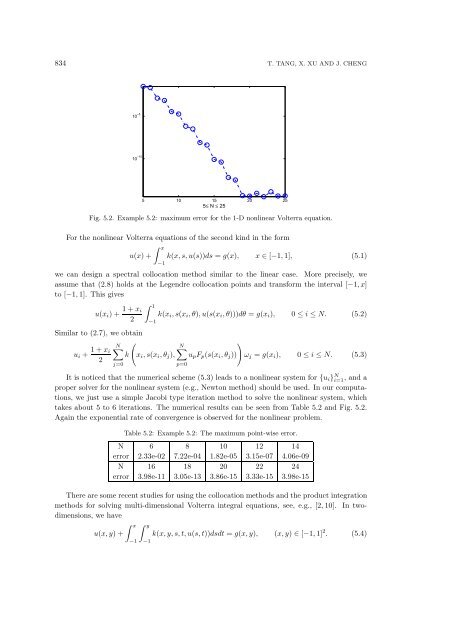
Fig. 5.2. Example 5.2: maximum error for the 1-D nonlinear Volterra equation.
For the nonlinear Volterra equations of the second kind in the form
u(x) +
∫ x
−1
k(x, s, u(s))ds = g(x), x ∈ [−1, 1], (5.1)
we can design a spectral collocation method similar to the linear case. More precisely, we
assume that (2.8) holds at the Legendre collocation points and transform the interval [−1, x]
to [−1, 1]. This gives
u(x i ) + 1 + x i
2
j=0
∫ 1
−1
k(x i , s(x i , θ), u(s(x i , θ)))dθ = g(x i ), 0 ≤ i ≤ N. (5.2)
Similar to (2.7), we obtain
(
)
u i + 1 + x N∑
N∑
i
k x i , s(x i , θ j ), u p F p (s(x i , θ j )) ω j = g(x i ), 0 ≤ i ≤ N. (5.3)
2
p=0
It is noticed that the numerical scheme (5.3) leads to a nonlinear system for {u i } N i=1 , and a
proper solver for the nonlinear system (e.g., Newton method) should be used. In our computations,
we just use a simple Jacobi type iteration method to solve the nonlinear system, which
takes about 5 to 6 iterations. The numerical results can be seen from Table 5.2 and Fig. 5.2.
Again the exponential rate of convergence is observed for the nonlinear problem.
Table 5.2: Example 5.2: The maximum point-wise error.
N 6 8 10 12 14
error 2.33e-02 7.22e-04 1.82e-05 3.15e-07 4.06e-09
N 16 18 20 22 24
error 3.98e-11 3.05e-13 3.86e-15 3.33e-15 3.98e-15
There are some recent studies for using the collocation methods and the product integration
methods for solving multi-dimensional Volterra integral equations, see, e.g., [2, 10]. In twodimensions,
we have
u(x, y) +
∫ x ∫ y
−1
−1
k(x, y, s, t, u(s, t))dsdt = g(x, y), (x, y) ∈ [−1, 1] 2 . (5.4)