

On Spectral Methods for Volterra Type Integral Equations and the ...
On Spectral Methods for Volterra Type Integral Equations and the ...
On Spectral Methods for Volterra Type Integral Equations and the ...

You also want an ePaper? Increase the reach of your titles
YUMPU automatically turns print PDFs into web optimized ePapers that Google loves.
<strong>On</strong> <strong>Spectral</strong> <strong>Methods</strong> <strong>for</strong> <strong>Volterra</strong> <strong>Integral</strong> <strong>Equations</strong> <strong>and</strong> <strong>the</strong> Convergence Analysis 835<br />
10 −4 5≤ N ≤ 20<br />
10 −6<br />
10 −8<br />
10 −10<br />
10 −12<br />
10 −14<br />
5 10 15 20<br />
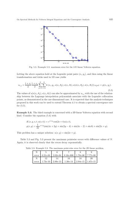
Fig. 5.3. Example 5.3: maximum error <strong>for</strong> <strong>the</strong> 2-D linear <strong>Volterra</strong> equation.<br />
Letting <strong>the</strong> above equation hold at <strong>the</strong> Legendre point pairs (x i , y j ), <strong>and</strong> <strong>the</strong>n using <strong>the</strong> linear<br />
trans<strong>for</strong>mation <strong>and</strong> tricks used in 1D case yields<br />
u i,j + 1 + x i<br />
2<br />
1 + x j<br />
2<br />
N∑<br />
p=0 l=0<br />
N∑<br />
k (x i , y j , s(x i , θ p ), s(x i , θ l ), u(s(x i , θ p ), s(x i , θ l ))) ω p ω l = g(x i , y j ).<br />
(5.5)<br />
The values of u(s(x i , θ p ), s(x i , θ l )) can also be approximated by u i,j with <strong>the</strong> use of <strong>the</strong> relationship<br />
between <strong>the</strong> Lagrange interpolation polynomials associate with <strong>the</strong> Legendre collocation<br />
points, as demonstrated in <strong>the</strong> one-dimensional case. It is expected that <strong>the</strong> analysis techniques<br />
proposed in this work can be used to extend Theorem 4.1 to obtain a spectral convergence rate<br />
<strong>for</strong> (5.5).<br />
Example 5.3. The third example is concerned with a 2D linear <strong>Volterra</strong> equation with second<br />
kind. Consider <strong>the</strong> equation (5.4) with<br />
K(x, y, s, t, u(s, t)) = e x+y cos(2s + t)u(s, t),<br />
g(x, y) = 1<br />
16 ex+y (sin(4x + 2y) + sin(2y − 4) + sin(4x − 2) + sin 6) + sin(2x + y).<br />
This problem has a unique solution: u(x, y) = sin(2x + y).<br />
Table 5.3 <strong>and</strong> Fig. 5.3 present <strong>the</strong> maximum pointwise errors with difference values of N.<br />
Again, it is observed clearly that <strong>the</strong> errors decay exponentially.<br />
Table 5.3: Example 5.3: The maximum point-wise error <strong>for</strong> <strong>the</strong> 2D linear problem.<br />
N 5 6 7 8 9<br />
error 6.21e-04 2.02e-04 8.16e-006 1.78e-06 7.77e-08<br />
N 12 14 16 18 20<br />
error 1.73e-10 2.89e-13 1.30e-14 2.94e-15 1.67e-15


