Obfuscation of Abstract Data-Types - Rowan

CHAPTER 1. OBFUSCATION 19
Then the relationship between A and B 1 and B 2 is given by the following rule:
{
B1 [f
A[i] = 1 (i)] if ch(i)
B 2 [f 2 (i)] otherwise
To ensure that there are no index clashes we require that f 1 is injective for the
values for which ch is true (similarly for f 2 ).
This relationship can be generalised so that A could be split between more
than two arrays. For this, ch should be regarded as a choice function — this
will determine which array each element should be transformed to.
We can write the transformation described in (1.3) as:
{
B1 [i div 2] if i is even
A[i] =
(1.4)
B 2 [i div 2] if i is odd
We will consider this obfuscation in much greater detail: in Section 2.3.7 we
give a specification of this transformation and in Chapter 4 we apply splits to
more general data-types.
1.3.7 Program transformation
We now show how we can transform a method using example (1.4) above. The
statement A[i] = V is transformed to:
if ((i%2) == 0) {B 1 [i/2] = V ; } else {B 2 [i/2] = V ; } (1.5)
and an occurrence of A[i] on the right hand side of an assignment can be dealt
with in a similar manner by substituting either B 1 [i/2] or B 2 [i/2] for A[i].
As a simple example, we present an imperative program for finding the first
n Fibonacci numbers:
A[0] = 0;
A[1] = 1;
i = 2;
while (i ≤ n)
{ A[i] = A[i−1] + A[i−2];
i + +;
}
In this program, we can easily spot the Fibonacci identity:
fib(0) = 0
fib(1) = 1
fib(n) = fib(n−1) + fib(n−2) (∀n ≥ 2)
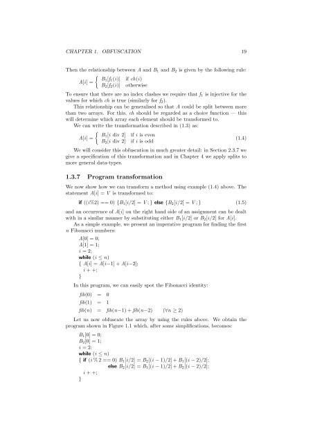
Let us now obfuscate the array by using the rules above. We obtain the
program shown in Figure 1.1 which, after some simplifications, becomes:
B 1 [0] = 0;
B 2 [0] = 1;
i = 2;
while (i ≤ n)
{ if (i %2 == 0) B 1 [i/2] = B 2 [(i − 1)/2] + B 1 [(i − 2)/2];
else B 2 [i/2] = B 1 [(i − 1)/2] + B 2 [(i − 2)/2];
i + +;
}