PhD Thesis Semi-Supervised Ensemble Methods for Computer Vision

50 Chapter 4. SemiBoost and Visual Similarity Learning
+
+
?
?
-
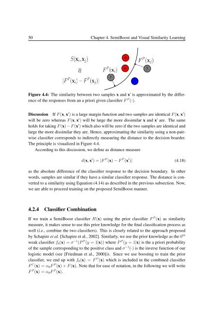
Figure 4.4: The similarity between two samples x and x ′ is approximated by the difference
of the responses from an a priori given classifier F P (·).
Discussion If F (x, x ′ ) is a large margin function and two samples are identical F (x, x ′ )
will be zero whereas F (x, x ′ ) will be large the more dissimilar x and x ′ are. The same
holds for taking F (x) − F (x ′ ) which also will be zero if the two samples are identical and
large the more dissimilar they are. Hence, approximating the similarity using a non-pairwise
classifier corresponds to indirectly measuring the distance to the decision boarder.
The principle is visualized in Figure 4.4.
According to this discussion, we define as distance measure
d(x, x ′ ) = |F P (x) − F P (x ′ )| (4.18)
as the absolute difference of the classifier response to the decision boundary. In other
words, samples are similar if they have a similar classifier response. The distance is converted
to a similarity using Equation (4.14) as described in the previous subsection. Now,
we are able to proceed training on the proposed SemiBoost manner.
4.2.4 Classifier Combination
If we train a SemiBoost classifier H(x) using the prior classifier F P (x) as similarity
measure, it makes sense to use this prior knowledge for the final classification process as
well (i.e., combine the two classifiers). This is closely related to the approach proposed
by Schapire et al. [Schapire et al., 2002]. Similarly, we use the prior knowledge as the 0 th
weak classifier f 0 (x) = σ −1 (P P (y = 1|x)) where P P (y = 1|x) is the a priori probability
of the sample corresponding to the positive class and σ −1 (·) is the inverse function of our
logistic model (see [Friedman et al., 2000])). Since we use boosting to train the prior
classifier, we end up with f 0 (x) = F P (x) which is included in the combined classifier
F C (x) = α 0 F P (x) + F (x). Note that for ease of notation, in the following we will write
F P (x) = α 0 F P (x).