PhD Thesis Semi-Supervised Ensemble Methods for Computer Vision

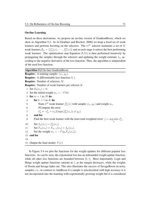
5.2. On Robustness of On-line Boosting 71
On-line Learning
Based on these derivations, we propose an on-line version of GradientBoost, which we
show in Algorithm 5.2. As in [Grabner and Bischof, 2006] we keep a fixed set of weak
learners and perform boosting on the selectors. The m th selector maintains a set of K
weak learners S m = {f 1 m(x), · · · , f K m (x)} and at each stage it selects the best performing
weak learners. The optimization step Equation (5.11) is then performed iteratively by
propagating the samples through the selectors and updating the weight estimate λ m according
to the negative derivative of the loss function. Thus, the algorithm is independent
of the used loss function.
Algorithm 5.2 On-line GradientBoost
Require: A training sample: (x n , y n ).
Require: A differentiable loss function l(·).
Require: Number of selectors M.
Require: Number of weak learners per selector K.
1: Set F 0 (x n ) = 0.
2: Set the initial weight w n = −l ′ (0).
3: for m = 1 to M do
4: for k = 1 to K do
5: Train k th weak learner fm(x) k with sample (x n , y n ) and weight w n .
6: //Compute the error
7: e k m ← e k m + w n I(sign(fm(x k n )) ≠ y n ).
8: end for
9: Find the best weak learner with the least total weighted error: j = arg min e k m.
k
10: Set f m (x n ) = fm(x j n ).
11: Set F m (x n ) = F m−1 (x n ) + f m (x n ).
12: Set the weight w n = −l ′ (y n F m (x n )).
13: end for
14:
15: Output the final model: F (x)
In Figure 5.4 we plot the functions for the weight updates for different popular loss
functions. As can be seen, the exponential loss has an unbounded weight update function,
while all other loss functions are bounded between [0, 1]. Most importantly, Logit and
Hinge weight update functions saturate at 1, as the margin decreases, while the weights
of Doom and Savage fades out. This also illustrates the success of SavageBoost on noisy
samples; i.e., in contrast to AdaBoost if a sample is misclassified with high accuracy it is
not incorporated into the learning with exponentially growing weight but it is considered