Alg 1 TE Lesson 10-8

2. Teach
Guided Instruction
1
Visual Learners
Help students remember the
general appearance of each
function by drawing the
following on the board:
2
EXAMPLE
q adratic
y ax sq ared bx c
e ponential
y a · b
inear
y mx b
EXAMPLE
Technology Tip
Students can use a graphing
calculator to graph the data,
determine the type of function
that best fits the data, and write
an equation to model the data.
Press
to enter the data
in lists. Press 2nd STAT PLOT
9 to graph the points.
You can see that the model is not
linear.
Quick Check
1
Graph each set of points. Which model is most appropriate for each set?
a. (-1.5, -2), (0, 2), (1, 4), (2, 6) b. (-1, 1), (0, 0), (1, 1), (2, 4)
c. (-1, 0.5), (0, 1), (1, 2), (2, 4) a–c. See margin.
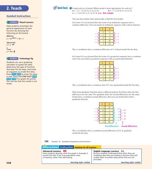
You can also analyze data numerically to find the best model.
In Lesson 5-6, you learned that the terms of an arithmetic sequence have a
common difference. You can model an arithmetic sequence with a linear function.
1
1
1
1
The y-coordinates have a common difference of 4. A linear model fits the data.
In Lesson 8-6, you learned that the terms of a geometric sequence have a common
ratio. You can model a geometric sequence with an exponential function.
1
1
1
1
x
2 2
1 2
0 6
1 10
x
2
1
0
The y-coordinates have a common ratio of 3. An exponential model fits the data.
y
2 14
y
1
9
1
3
1
1 3
2 9
4
4
4
4
3
3
3
3
Data from quadratic functions show a different pattern. For linear data, the first
differences are the same. For quadratic data, the second differences are the same.
If data have a common second difference, then you can model them with a
quadratic function.
x
y
1
1
1
1
1
1 16
0 2
1 2
2 4
3 20
4 46
14
4
6
16
26
10
10
10
10
first differences
second differences
The y-coordinates have a common second difference of 10. A quadratic
model fits the data.
598 Chapter 10 Quadratic Equations and Functions
598
Advanced Learners L4
Have students describe what the graph in Example 3
would look like if the frog population were
increasing, rather than decreasing.
learning style: verbal
English Language Learners ELL
Be sure students understand that when they are
modeling data they are finding a function that will
enable them to predict data points that are not
provided.
learning style: verbal