Alg 1 TE Lesson 10-8

10-8
What You’ll Learn
• To choose a linear,
quadratic, or exponential
model for data
. . . And Why
To model changes in an
animal population, as in
Example 3
Choosing a Linear, Quadratic,
or Exponential Model
Check Skills You’ll Need GO for Help
Graph each function. 1–6. See margin p. 599.
1. y = 3x - 1 2. y =
1
4 x + 2
3. y = 2 x 4. y = Q 1 3 Rx
5. y = x 2 + 5 6. y = 2x 2 - 1
Lessons 6-2, 8-7, and 10-1
10-8
1. Plan
Objectives
1 To choose a linear, quadratic,
or exponential model for data
Examples
1 Choosing a Model by
Graphing
2 Modeling Data
3 Real-World Problem Solving
Math Background
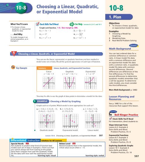
Part 1 1 Choosing a Linear, Quadratic, or Exponential Model
You can use the linear, exponential, or quadratic functions you have studied to
model some sets of data. Recall the general appearance of each type of function.
Key Concepts Summary Linear, Quadratic, and Exponential Functions
Linear Quadratic Exponential
y = mx + b y = ax 2 + bx + c y = a ? b x
y
O
x
y
O
x
y
O
x
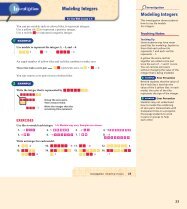
You can test ordered data for a
common difference or common
ratio. A linear model fits data
with a common difference and
an exponential model fits data
with a common ratio. A quadratic
model fits data with common
second differences. (Second
differences are differences of the
first differences.) To find the
second differences to determine
quadratic models remember that
x will be squared. To determine
cubic models, you must consider
the third differences.
More Math Background: p. 548D
1
You may be able to use the graph of data points to determine a model for the data.
EXAMPLE
Choosing a Model by Graphing
Graph each set of points. Which model is most appropriate for each set?
a. (-3, 6), (-2, 2), (0, -2), b. (-2, 5), (0, 3), c. (-2, 4), (-1, 2),
(3, 6), (1, -1), (2, 2) (1, 2.5), (2, 2) (1, -2), (2, -4)
y
6
y
5
y
6
4
4
4
64
2
x
3
x
2
O 2 4 6
64
O 2 4 6
1
x
4
4
32
O 1 2 3
Quadratic model Exponential model Linear model
Lesson Planning and
Resources
See p. 548E for a list of the
resources that support this lesson.
PowerPoint
Bell Ringer Practice
Check Skills You’ll Need
For intervention, direct students to:
Slope-Intercept Form
Lesson 6-2: Example 4
Extra Skills and Word
Problem Practice, Ch. 6
Lesson 10-8 Choosing a Linear, Quadratic, or Exponential Model 597 Exponential Functions
Lesson 8-7: Example 3
Extra Skills and Word
Special Needs L1
Below Level L2
Problem Practice, Ch. 8
Ask students to predict what kind of function best Remind students that in the exponential model, the Exploring Quadratic Graphs
models each set of data in Example 2. Point out that initial value occurs when x = 0.
Lesson 10-1: Example 4
you cannot always tell from looking at the graph.
Extra Skills and Word
Have them compare how well the quadratic model
Problem Practice, Ch. 10
fits the data with how well the exponential model
fits.
learning style: visual learning style: verbal
597

2. Teach
Guided Instruction
1
Visual Learners
Help students remember the
general appearance of each
function by drawing the
following on the board:
2
EXAMPLE
q adratic
y ax sq ared bx c
e ponential
y a · b
inear
y mx b
EXAMPLE
Technology Tip
Students can use a graphing
calculator to graph the data,
determine the type of function
that best fits the data, and write
an equation to model the data.
Press
to enter the data
in lists. Press 2nd STAT PLOT
9 to graph the points.
You can see that the model is not
linear.
Quick Check
1
Graph each set of points. Which model is most appropriate for each set?
a. (-1.5, -2), (0, 2), (1, 4), (2, 6) b. (-1, 1), (0, 0), (1, 1), (2, 4)
c. (-1, 0.5), (0, 1), (1, 2), (2, 4) a–c. See margin.
You can also analyze data numerically to find the best model.
In Lesson 5-6, you learned that the terms of an arithmetic sequence have a
common difference. You can model an arithmetic sequence with a linear function.
1
1
1
1
The y-coordinates have a common difference of 4. A linear model fits the data.
In Lesson 8-6, you learned that the terms of a geometric sequence have a common
ratio. You can model a geometric sequence with an exponential function.
1
1
1
1
x
2 2
1 2
0 6
1 10
x
2
1
0
The y-coordinates have a common ratio of 3. An exponential model fits the data.
y
2 14
y
1
9
1
3
1
1 3
2 9
4
4
4
4
3
3
3
3
Data from quadratic functions show a different pattern. For linear data, the first
differences are the same. For quadratic data, the second differences are the same.
If data have a common second difference, then you can model them with a
quadratic function.
x
y
1
1
1
1
1
1 16
0 2
1 2
2 4
3 20
4 46
14
4
6
16
26
10
10
10
10
first differences
second differences
The y-coordinates have a common second difference of 10. A quadratic
model fits the data.
598 Chapter 10 Quadratic Equations and Functions
598
Advanced Learners L4
Have students describe what the graph in Example 3
would look like if the frog population were
increasing, rather than decreasing.
learning style: verbal
English Language Learners ELL
Be sure students understand that when they are
modeling data they are finding a function that will
enable them to predict data points that are not
provided.
learning style: verbal

x y
1 20
0 8
1 3.2
2 1.28
3 0.512
2
EXAMPLE
Modeling Data
a. Which kind of function best models the data at the left? Write an equation to
model the data.
Step 1 Graph the data.
8
7
6
5
4
3
2
1
O
y
x
1 2 3 4 5 6 7 8 9
1
1
1
1
Step 2 The data appear to suggest an
exponential model. Test for a
common ratio.
x
1
0
1
2
3
20
8
There is a common ratio, 0.4.
y
3.2
1.28
0.512
8 20 0.4
3.2 8 0.4
1.28 3.2 0.4
0.512 1.28 0.4
To determine if a quadratic or
exponential function best models
the data, use the calculator to
find each equation that best fits
the data. Press 5
Y= 5 .
The quadratic model will appear
on the graph. To find the
exponential model, follow the
same steps except press 0 instead
of the first 5, and scroll to Y 2 =
after you press Y= . Now the
exponential model will appear.
The exponential model passes
through more of the data
points. Press Y= and write
the exponential equation after
Y 2 as y = 8 ? 0.4 x .
Step 3 Write an exponential model. Step 4 Test two points other than (0, 8).
Relate y = a ? b x y = 8 ? 0.4 1 y = 8 ? 0.4 3
PowerPoint
Additional Examples
x y
0 0
1 0.3
2 1.2
3 2.7
4 4.8
Define Let a = the initial value, 8. y = 8 ? 0.4 y = 8 ? 0.064
Let b = the decay factor, 0.4. y = 3.2 y = 0.512
Write y = 8 ? 0.4 x (1, 3.2) and (3, 0.512) are both data points.
The equation y = 8 ? 0.4 x models
the data.
b. Which kind of function best models the data at the left? Write an equation to
model the data.
Step 1 Graph the data.
6
5
4
3
2
1
2 O
2
y
x
1 2 3 4 5 6 7 8
Step 2 The data appear to be quadratic.
Test for a common second
difference.
1
1
1
1
x
0
1
0
y
0.3
2 1.2
3 2.7
4 4.8
0.3
0.9
1.5
2.1
0.6
0.6
0.6
There is a common second difference, 0.6.
1 Graph each set of points.
Which model is most appropriate
for each set?
a. (-2, 1.45), (0, 3), (1, 4) (2, 6)
exponential
b. (-2, -2), (0, 2), (1, 4), (2, 6)
linear
c. (-2, 11), (-1, 5), (0, 3), (1, 5),
(2, 11) quadratic
6.
2
page 598 Quick Check
1a. y linear
6
y
4
2
O
x
2
Step 3 Write a quadratic model. Step 4 Test two points other than
(2, 1.2) and (0, 0).
y = ax 2 y = 0.3(3) 2 y = 0.3(4) 2
1.2 = a(2) 2 Use a point other
than (0, 0) to find a.
y = 0.3 ? 9 y = 0.3 ? 16
y = 2.7 y = 4.8
1.2 = 4a Simplify.
0.3 = a Divide each side by 4. (3, 2.7) and (4, 4.8) are both data points.
y = 0.3x 2 Write a quadratic The equation y = 0.3x 2 models the data.
function.
4
2
O
2
b. y quadratic
4
x
2
2
Lesson 10-8 Choosing a Linear, Quadratic, or Exponential Model 599
O
x
2
page 597 Check Skills You’ll Need
1. y 2. y
3. y
4. y 5.
2
O x
1 1
1
2 O 2
x
2
8
4
O
2
x
2
8
4
O
x
1
2
y
8
4
O
x
2
c. y exponential
4
2
x
O 2
599

PowerPoint
Additional Examples
2 Which kind of data best
models the data below? Write
an equation to model the data.
a.
x y
0 0
1 1.4
2 5.6
3 12.6
4 22.4
b.
quadratic; y ≠ 1.4x 2
x
-1 4
0 2
1 1
exponential; y ≠ 2 ? 0.5 x
3 Suppose you are studying deer
that live in an area. The data
below were collected by a local
conservation organization. It
indicates the number of deer
estimated to be living in the area
over a five-year period. Determine
which kind of function best
models the data. Write an
equation to model the data.
exponential; y ≠ 90 ? 0.77 x
Resources
• Daily Notetaking Guide 10-8
L3
• Daily Notetaking Guide 10-8—
Adapted Instruction L1
Closure
y
2 0.5
3 0.25
Estimated
Year Population
0 90
1 69
2 52
3 40
4 31
Real-World
Quick Check
Connection
Frog populations around the
world have been declining
over the past 20 years.
2
3
Which kind of function best models the data in each table? Write an equation to
model the data.
a.
x y
b.
x y
c.
x y
0 4
1
0
0 0
2
1 4.4
1 1
1 0.5
2 4.84
1
2 2
2 1
2
3 5.324
3 4.5
3 2
4 5.8564
4 8
exponential; y ≠ 4 ? 1.1 x 1 1
linear; y ≠ x ± quadratic; y ≠– 1 x 2
2 2
2
While real-world data seldom fall exactly into linear, exponential, or quadratic
patterns, you can find a best-possible model.
EXAMPLE Real-World Problem Solving
Zoology Suppose you are studying frogs that live in a
nearby wetland area. The data at the right were collected by
a local conservation organization. They indicate the number
of frogs estimated to be living in the wetland area over a
five-year period. Determine which kind of function best
models the data. Write an equation to model the data.
Step 1 Graph the data to decide which model is
most appropriate.
Population
Step 2 Test for a common ratio.
1
1
1
1
120
80
40
0
1 2 3 4 5 6
Year
Year
0
1
2
3
4
Estimated
Population
120
101
86
72
60
The graph curves, and it does not look
quadratic. It may be exponential.
The population of frogs is roughly 0.84 times its value the previous year.
Step 3 Write an exponential model.
Relate y = a ? b x
Define Let a = the initial value, 120.
Let b = the decay factor, 0.84.
Write y = 120 ? 0.84 x
101 120 0.84
86 101 0.85
72 86 0.84
60 72 0.83
Year
0
1
2
3
4
The common ratio is
roughly 0.84.
Estimated
Population
120
101
86
72
60
Ask students how to choose a
linear, quadratic, or exponential
model for data. First graph the
data to see if the graph is linear
or if it curves. Then look for a
best fit model.
600 Chapter 10 Quadratic Equations and Functions
600

Quick Check
EXERCISES
Practice and Problem Solving
A
GO
Practice by Example
for
Help
Example 1
(page 597)
Step 4 Test two points other than (0, 120).
y = 120 ? 0.84 3 y = 120 ? 0.84 4
y < 71 y < 60
The point (3, 71) is close to the data point (3, 72). The predicted value (4, 60)
matches the corresponding data point. The equation y = 120 ? 0.84 x models
the data.
Year Profit (dollars)
3 The profits of a small company are shown
0
0
in the table at the right. Let x = 0 correspond
1 5,000
to the year 2000.
2 20,000
a. Determine which kind of function best models
the data. quadratic
3 44,000
b. Write an equation to model the data. y ≠ 5000x 2 4 79,000
For more exercises, see Extra Skill and Word Problem Practice.
1–6. See
Graph each set of points. Which model is most appropriate for each set? back of
book.
1. (-2, -3), (-1, 0), (0, 1), (1, 0), (2, -3) 2. (-2, -8), (0, -4), (3, 2), (5, 6)
3. (-3, 6), (-1, 0), (0, -1), (1, -1.5) 4. (-2, 5), (-1, -1), (0, -3), (1, -1), (2, 5)
5. Q-2, 25
8
, -1, 25
2
9
R Q
3
R, (0, -5), (2, 3) 6. (-3, 8), (-1, 6), (0, 5), (2, 3), (3, 2)
3. Practice
Assignment Guide
1
A B 1-27
C Challenge 28-29
Test Prep 30-33
Mixed Review 34-48
Homework Quick Check
To check students’ understanding
of key skills and concepts, go over
Exercises 8, 14, 17, 18, 20.
Error Prevention!
Exercises 1–6 Be sure students do
not quickly determine that the
best model is exponential as soon
as they see that the graph is not
linear. They need to graph all
points to see if the graph is a
quadratic model.
Example 2
(page 599)
Example 3
(page 600)
Which kind of function best models the data in each table? Write an equation to
model the data.
7. x y
8. x y
9. x y
0 0
0 5
0 0
1 1.5
1 3
1 2.8
2 6
2 1
2 11.2
3 13.5
3 1
3 25.2
4 24
4 3
4 44.8
quadratic; y ≠ 1.5x 2 linear; y ≠ 2x – 5 quadratic; y ≠ 2.8x 2
10. x y 11. x y 12. x y
0
1
1 1.2
2 1.44
3 1.728
0
5
1 2
2 0.8
3 0.32
4 2.0736
4 0.128
4 0
exponential; y ≠ 1 ? 1.2 x exponential; y ≠ 5 ? 0.4 x 1
linear; y ≠– 2 x ± 2
13. The table at the right shows the end-of-themonth
balance in a checking account.
Month Balance (dollars)
a. Graph the data. Does the graph suggest a
linear, exponential, or quadratic model?
1
2
58
123
b. Find the differences of consecutive terms.
3
187
Are they roughly the same? 65, 64, 64; yes
c. Estimate a common difference based on
4
251
your answer to part (b). 64
d. Write an equation to model the data. y ≠ 64x – 5
a. See back of book.
0
2
1 1.5
2 1
3 0.5
Lesson 10-8 Choosing a Linear, Quadratic, or Exponential Model 601
GPS
Enrichment
Guided Problem Solving
Reteaching
Adapted Practice
Practice
© Pearson Education, Inc. All rights reserved.
Name Class Date
Practice 10-9
Choosing a Linear, Quadratic, or Exponential Model
Which kind of function best models the data? Write an equation to model
the data.
1. (-1, 3), (1, 3), (3, 27), (5, 75), (7, 147) 2. (-2, 4), (-1, 2), (0, 0), (1, -2), (2, -4)
3. ¢ 22, ≤, ¢ 21, 1 ≤, (0, 1), (1, 4), (2, 16) 4. (-6, -1), (-3, 0), (0, 1), (3, 2), (6, 3)
16
1 4
5. ¢ 22, 1 3
≤,(-1, 1), (0, 3), (1, 9), (2, 27) 6. (-4, -32), (-2, -8), (0, 0), (2, -8), (4, -32)
7. 8. 9.
x y
x y
-3
9
2
-2 2
1
-1
2
0 0
10. 11. 12.
x y
x y
0 -2
1 -8
2 -32
3 -128
13. ¢ 22, ≤, ¢ 21, ≤, ¢ 0, 1 ≤, ¢ 1, 1 ≤, ¢ 2, 1 ≤
3
1 1 3 3 3 3
14. ¢ 21, 2 1 ≤, ¢ 0, 2 1 ≤, (1, -1), (2, -2), (3, -4)
4 2
15. The cost of shipping computers from a warehouse is given in the table below.
Number of Computers 50 75 100 125
Cost (dollars) 1700 2500 3300 4100
a. Determine which kind of function best models the data.
b. Write an equation to model the data.
-1 -2
0 -4
1 -6
2 -8
-7 -245
-5 -125
-3 -45
-1 -5
c. On the basis of your equation, what is the cost of shipping 27 computers?
d. On the basis of your equation, how many computers could be shipped for $5500?
16. During a scientific experiment, the bacteria count was taken at 5-min intervals.
The data shows the count at several time periods during the experiment.
Time Interval 0 1 2 3
Count 110 132 159 190
a. Determine which kind of function best models the data.
b. Write an equation to model the data.
c. On the basis of your equation, what is the count 1 hr, 45 min after the start
of the experiment?
x
y
-4 -4
-2 -1
x
-2
0 0
2 -1
0
y
3
2
1
2
1
2 -
2
4 -
2
3
L4
L1
L3
L2
L3
601

Math Tip
Exercises 19–24 Remind students
that r is the correlation coefficient.
The nearer r is to 1 or -1, the
more closely the data cluster
around the model. The closer r is
to 1 or - 1, the greater r 2 is.
Also, the TI-83 Plus does not
automatically show r-values for
regressions. This feature, under
catalog, is called DiagnosticsOn,
and needs to be highlighted and
switched on for this to happen.
pages 563–566
16a. p
602
Exercises
linear
18. Answers may vary.
Sample: Linear data
have a common first
difference, quadratic
data have a common
second difference, and
exponential data have a
common ratio.
25a. i. x y
29f.
Population
ii.
iii.
Sales (billions of dollars)
6000
4000
2000
O
1 –2
2 1
3 6
4 13
5 22
x y
1 3
2 12
3 27
4 48
5 75
x y
1 –1
2 6
3 21
4 44
5 75
y
800
700
600
500
400
300
200
100
O
t
4 8 12 16
Year
)3 )2
)5 )2
)7 )2
)9
) 9 )6
)15 )6
)21 )6
)27
) 7 )8
)15 )8
)23 )8
)31
x
5 10 15 20
Year
Age
(years)
B
Value
(dollars)
0 16,500
1 14,500
2 12,750
3 11,200
4 9900
Apply Your Skills
16c. 600, 600, 600;
120, 120, 120
Population
Year (millions)
0 4457
5 4855
10 5284
15 5691
20 6080
SOURCES: U. S. Census Bureau.
Go to www.PHSchool.com
for a data update.
Web Code: atg-9041
GO
nline
Homework Help
Visit: PHSchool.com
Web Code: ate-1008
14. Car Value The value of a car over several years is shown in the table at the left.
a. Determine which model is most appropriate for the data. exponential
b. Write an equation to model the data. y ≠ 16,500 ? 0.88 x
15. Physics Your class collected the data in the table
at the right by rolling a ball down a ramp. The
ramp had the same angle throughout. a. 41, 123, 206
a. Find the differences of consecutive terms.
b. Find the second differences. 82, 83
c. Write an equation to model the data. Let t
be the time in seconds and d be the distance
in centimeters. d ≠ 41t 2
d. Based on your equation, how far would the ball have rolled down the ramp
in 2.5 seconds? 256.25 cm
16. The table below shows the projected population of a small town. Let t = 0
correspond to the year 2020. a. See margin.
a. Graph the data. Does the graph suggest a
linear, exponential, or quadratic model?
Year Population
b. What is the difference in years? 5 years
0 5100
c. Find the differences of consecutive terms.
5 5700
Divide by the difference in years to find
10 6300
possible common differences. See left.
15 6900
d. Write a linear equation to model the data
based on your answer to part (c). p ≠ 120t ± 5100
17. Population The table at the left shows the world population in millions from
GPS 1980 to 2000. The year t = 0 corresponds to 1980.
a. What is the difference in years? 5
b. Find the differences of consecutive terms. Divide by the difference in years
to find possible common differences. 398, 429, 407, 389; 79.6, 85.8, 81.4, 77.8
c. Find the average of the common differences you found in part (b). about 81.2
d. Write a linear equation to model the data based on your answer to part (c).
e. Use your equation to predict the world population in 2010.
d. p ≠ 81.2t ± 4457 e. 6893 million, or about 6.9 billion
18. Writing Explain in writing to a classmate how to decide whether a linear,
exponential, or quadratic function is the most appropriate equation to model
a set of data. See margin.
Use LinReg, ExpReg, or QuadReg to find an equation to model the data.
The greatest value of r 2 indicates the best model for the data.
19. x y 20. x y 21. x y
0 1.7
1 1.4
2 4.7
3
y ≠ 0.875x 2 – 0.435x ± 1.515 y ≠ 1.987 ? 0.770 x y ≠ 2.125x 2 – 4.145x ± 2.955
22. x y 23. x y 24. x y
1
7.9
4.3
0 5.1
1 4.3
2 2.2
0 2.0
1 1.5
2 1.2
3
1
0 3.5
3 1.3
3 0.2
3 1.76
y ≠–0.336x 2 – 0.219x ± 4.666 y ≠–1.1x ± 3.5 y ≠ 0.102 ? 2.582 x
602 Chapter 10 Quadratic Equations and Functions
0.9
4.6
1 2.4
2 1.3
Time
(seconds)
0 0
1 41
2 164
3 370
0 2.8
1 1.4
2 2.7
3
1
Distance
(centimeters)
9.8
0.04
0 0.10
1 0.26
2 0.68

25b. The second
common difference
is twice the
coefficient of x 2 .
25c. When second
differences are the
same, the data are
quadratic. You can
determine the
coefficient of x 2 by
dividing the second
difference by 2.
26. Answers may vary.
Sample: x y
0 5
2 13
4 29
6 53
C
Challenge
29c. –54, 89, 66
d. 1.85; the ratio is
much greater than
the other ratios.
e. Yes; if consecutive
first differences
decrease, a second
difference will be
negative.
25. a. Make a table of five points using consecutive x-values for each function.
Find the common second difference. See margin.
i. f(x) = x 2 - 3 ii. f(x) = 3x 2 iii.f(x) = 4x 2 - 5x
b. What is the relationship between the common second difference and the
coefficient of x 2 ? See left.
c. Critical Thinking Explain how you could use this relationship to help you
model data if the function were not given. See left.
26. Open-Ended Write a set of data you could model with a quadratic function.
See left.
27. Physics A group of students dropped ping-pong balls and found the distance
the balls traveled, given a certain amount of time. The diagram below shows
their results.
a. Determine which
model is most
appropriate for
the data. quadratic
b. Write an equation to
model the data. If
necessary, round to
the nearest tenth.
c. Use your equation to
predict the distance a
ping-pong ball would
fall in 2 s. 54.5 ft
Answers may vary.
Sample: d ≠ 13.6t 2
0.2 s
0.5 ft
0.4 s
2.2 ft
28. Data Collection Complete the chart at the right for
your town. a–c. Check students’ work.
a. Use ExpReg or QuadReg to find an equation to
model the data.
b. Use the equation you found in part (a) to predict
the current population of your town.
c. Use the equation you found in part (a) to predict
the population of your town in 2010.
0.6 s
4.9 ft
29. Data Analysis There are times when data show trends but not consistent ratios
or differences. The data in the table below show the total U.S. retail auto sales
for the years 1980 through 2000.
The value t = 0 corresponds to the
United States Retail Auto Sales
year 1980. 1.85, 1.28, 1.45, 1.43
$802
a. Find the ratios of consecutive
entries in the sales columns.
Round to the nearest hundredth.
b. Find the differences of
1 car = $1 billion $562
consecutive entries in the sales
in sales
columns. 139, 85, 174, 240
$388
c. Find the second differences
of consecutive entries in the
$164
sales column. c–e. See left.
d. Which ratio is most different
from the others? Explain.
0 5 10 15 20
e. Critical Thinking If sales data
Year
increase every year, can a second
difference be negative? Explain.
f. Graph the data. Draw a curve to show the trend. See margin.
lesson quiz, PHSchool.com, Web Code: ata-1008 Lesson 10-8 Choosing a Linear, Quadratic, or Exponential Model 603
$303
0.8 s
8.7 ft
1.0 s
13.6 ft
Population
Year (thousands)
1970 7
1980 7
1990 7
2000 7
4. Assess & Reteach
Lesson Quiz
Which kind of function best
models the data in each table?
Write an equation to model the
data.
1.
x y
-1 15
2.
PowerPoint
0 3
1 0.6
2 0.12
3 0.024
exponential; y ≠ 3 ? 0.2 x
x y
-1 -5
0 -3
1 -1
2 1
3 3
linear; y ≠ 2x – 3
3.
x y
-1 2.2
0 0
1 2.2
2 8.8
3 19.8
quadratic; y ≠ 2.2x 2
Alternative Assessment
Have each student graph either a
linear, quadratic, or exponential
function, and then write four
points that are on the graph.
Instruct students to exchange the
set of points with a classmate. The
classmate finds the function that
best models the set of points, and
then writes an equation to model
the data. Direct students to
exchange the set of points with
another classmate and repeat.
Students can compare their
results.
603

Test Prep
Resources
For additional practice with a
variety of test item formats:
• Standardized Test Prep, p. 611
• Test-Taking Strategies, p. 606
• Test-Taking Strategies with
Transparencies
Exercise 31 Remind students that
the y-coordinates of an exponential
model have a common ratio. After
determining that the x-coordinates
are written in sequential order
with a common difference,
students just need to check the
first three y-coordinates of each
set of data to find the set with a
common ratio.
pages 601–604 Exercises
33. [4] a. linear
b. d ≠–2.5n ± 43.5
c. 18
[3] appropriate methods,
but with one
computational error
[2] part (c) not answered
[1] no work shown
37.
O y
2
x
2
Standardized Test Prep Test Prep
Multiple Choice
Short Response
Extended Response
30. Which equation best
models the data in the
table at the right? B
A. y = 4x
B. y = 2x + 2
C. y = 2 x
D. y = 2x 2
31. Which of the following sets of data is best described by an
exponential model? H
F. (-1, 16), Q2
1
2
, 4 R, (0, 2), Q 1 2
, -2 R, (1, 4) 32. [2] p ≠ 33,500(1.014) n ,
G. (1, -7), (2, -4), (3, -1), (4, 2), (5, 5)
33,500(1.014) 10 N
H. (1, 1), (3, 3), (0, 0.5), (5, 8), (7, 14)
38,497
J. (-2, -4), (-1, 3), (0, 8), (1, 14), (2, 12) [1] correct formula,
inaccurate evaluation
32. The population of a town was 33,500 in 2000. The population is
increasing by about 1.4% each year. Write an equation that will
predict the population n years after 2000. Let 2000 correspond to n = 0.
Predict the town’s population in 2010. See above.
33. Suppose you put marbles into a cup hanging from an elastic band (spring).
You measure the distance d from the floor in centimeters as the number n
of marbles is increased.
n 0
d 43.5
1
41
x
0
1
2
2
38.5
a. Which type of model best fits this data set? a–c. See margin.
b. Write an equation for the data.
c. Suppose the pattern shown above continues. Find the least number of
marbles you need to make the cup rest on the floor.
y
2
4
6
3 8
4 10
3
36
4
33.5
5
31
3
38.
f(x)
2
Mixed Review
39.
2 O 2
f(x)
6
2
O x
1 1
x
GO
for
Help
Lesson 10-7
Lesson 10-1
Lesson 8-7
Find the number of x-intercepts of each function.
34. y =-x 2 1 35. y = x 2 + 3x + 4 0 36. y = 4x 2 - 10x + 3 2
Graph each function. 37–42. See margin.
37. y =-2x 2 38. f(x) =
1
4
x 2 39. f(x) = x 2 + 4
40. y =-x 2 - 2 41. y = 3x 2 + 1 42. y =-
1
2
x 2 + 1
Evaluate each function rule for the given value.
43. y = 2 x for x =-3 0.125 44. f(x) =-2 x for x = 5 –32
40.
O y x
1 1
45. g(t) = 2 ? 3 t 2
for t =-3 46. f(t) = 10 ? 5 t 27
for t = 2 250
47. y = Q 1 2 Rt for t =-4 16 48. y = 9 ? Q 3 2 Rx for x = 3 30.375
4
604 Chapter 10 Quadratic Equations and Functions
41.
8
4
y
42.
y
O
1 1
x
x
1O
1
2
604