Estimators based in adaptively trimming cells in the mixture model
Estimators based in adaptively trimming cells in the mixture model
Estimators based in adaptively trimming cells in the mixture model

You also want an ePaper? Increase the reach of your titles
YUMPU automatically turns print PDFs into web optimized ePapers that Google loves.
( 16<br />
Σ 1 =<br />
0<br />
) (<br />
0<br />
8.5<br />
, Σ 2 =<br />
16 −7.5<br />
) (<br />
−7.5 1<br />
, Σ 3 =<br />
8.5<br />
0<br />
)<br />
0<br />
.<br />
1<br />
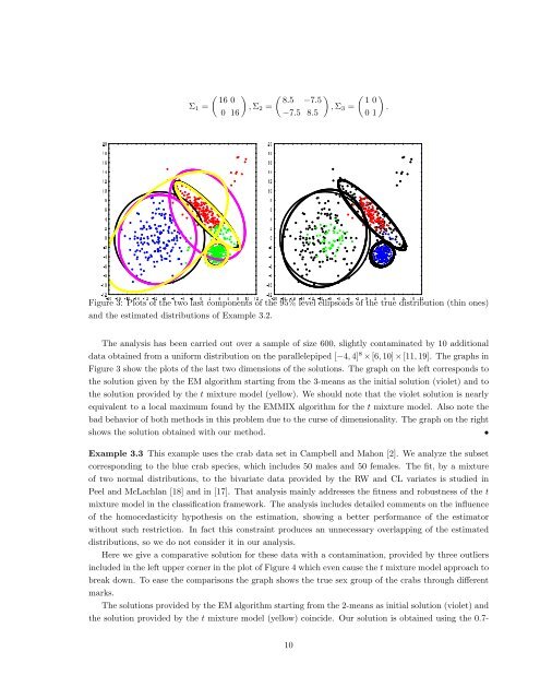
Figure 3: Plots of <strong>the</strong> two last components of <strong>the</strong> 95% level ellipsoids of <strong>the</strong> true distribution (th<strong>in</strong> ones)<br />
and <strong>the</strong> estimated distributions of Example 3.2.<br />
The analysis has been carried out over a sample of size 600, slightly contam<strong>in</strong>ated by 10 additional<br />
data obta<strong>in</strong>ed from a uniform distribution on <strong>the</strong> parallelepiped [−4, 4] 8 × [6, 10] × [11, 19]. The graphs <strong>in</strong><br />
Figure 3 show <strong>the</strong> plots of <strong>the</strong> last two dimensions of <strong>the</strong> solutions. The graph on <strong>the</strong> left corresponds to<br />
<strong>the</strong> solution given by <strong>the</strong> EM algorithm start<strong>in</strong>g from <strong>the</strong> 3-means as <strong>the</strong> <strong>in</strong>itial solution (violet) and to<br />
<strong>the</strong> solution provided by <strong>the</strong> t <strong>mixture</strong> <strong>model</strong> (yellow). We should note that <strong>the</strong> violet solution is nearly<br />
equivalent to a local maximum found by <strong>the</strong> EMMIX algorithm for <strong>the</strong> t <strong>mixture</strong> <strong>model</strong>. Also note <strong>the</strong><br />
bad behavior of both methods <strong>in</strong> this problem due to <strong>the</strong> curse of dimensionality. The graph on <strong>the</strong> right<br />
shows <strong>the</strong> solution obta<strong>in</strong>ed with our method.<br />
•<br />
Example 3.3 This example uses <strong>the</strong> crab data set <strong>in</strong> Campbell and Mahon [2]. We analyze <strong>the</strong> subset<br />
correspond<strong>in</strong>g to <strong>the</strong> blue crab species, which <strong>in</strong>cludes 50 males and 50 females. The fit, by a <strong>mixture</strong><br />
of two normal distributions, to <strong>the</strong> bivariate data provided by <strong>the</strong> RW and CL variates is studied <strong>in</strong><br />
Peel and McLachlan [18] and <strong>in</strong> [17]. That analysis ma<strong>in</strong>ly addresses <strong>the</strong> fitness and robustness of <strong>the</strong> t<br />
<strong>mixture</strong> <strong>model</strong> <strong>in</strong> <strong>the</strong> classification framework. The analysis <strong>in</strong>cludes detailed comments on <strong>the</strong> <strong>in</strong>fluence<br />
of <strong>the</strong> homocedasticity hypo<strong>the</strong>sis on <strong>the</strong> estimation, show<strong>in</strong>g a better performance of <strong>the</strong> estimator<br />
without such restriction. In fact this constra<strong>in</strong>t produces an unnecessary overlapp<strong>in</strong>g of <strong>the</strong> estimated<br />
distributions, so we do not consider it <strong>in</strong> our analysis.<br />
Here we give a comparative solution for <strong>the</strong>se data with a contam<strong>in</strong>ation, provided by three outliers<br />
<strong>in</strong>cluded <strong>in</strong> <strong>the</strong> left upper corner <strong>in</strong> <strong>the</strong> plot of Figure 4 which even cause <strong>the</strong> t <strong>mixture</strong> <strong>model</strong> approach to<br />
break down. To ease <strong>the</strong> comparisons <strong>the</strong> graph shows <strong>the</strong> true sex group of <strong>the</strong> crabs through different<br />
marks.<br />
The solutions provided by <strong>the</strong> EM algorithm start<strong>in</strong>g from <strong>the</strong> 2-means as <strong>in</strong>itial solution (violet) and<br />
<strong>the</strong> solution provided by <strong>the</strong> t <strong>mixture</strong> <strong>model</strong> (yellow) co<strong>in</strong>cide. Our solution is obta<strong>in</strong>ed us<strong>in</strong>g <strong>the</strong> 0.7-<br />
10