Estimators based in adaptively trimming cells in the mixture model
Estimators based in adaptively trimming cells in the mixture model
Estimators based in adaptively trimming cells in the mixture model
Create successful ePaper yourself
Turn your PDF publications into a flip-book with our unique Google optimized e-Paper software.
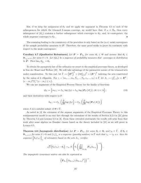
But, if we keep <strong>the</strong> uniqueness of θ P and we apply <strong>the</strong> argument <strong>in</strong> Theorem 4.5 to each of <strong>the</strong><br />
subsequences for which <strong>the</strong> trimmed k-means converge, we would have that, if ω ∈ Ω 0 , <strong>the</strong>n every<br />
subsequence of {ˆθ n } conta<strong>in</strong>s a fur<strong>the</strong>r subsequence which converges to θ P , and, <strong>in</strong> consequence, <strong>the</strong><br />
whole sequence converges to θ P .<br />
•<br />
The reason<strong>in</strong>g lead<strong>in</strong>g to <strong>the</strong> consistency of <strong>the</strong> procedure is only <strong>based</strong> on <strong>the</strong> (a.s.) weak convergence<br />
of <strong>the</strong> sample probability measures to IP . Therefore, <strong>the</strong> same proof works to prove its cont<strong>in</strong>uity with<br />
respect to <strong>the</strong> weak convergence:<br />
Corollary 4.7 (Qualitative Robustness) Let IP = IP θ0 for some θ 0 ∈ Θ and assume that θ 0 ∈<br />
Θ γP ,u+δ, for some δ > 0. Let {Q n } be a sequence of probability measures that converges <strong>in</strong> distribution<br />
to IP . Then lim n θ Qn = θ 0 .<br />
To obta<strong>in</strong> <strong>the</strong> asymptotic law of <strong>the</strong> estimator we resort to <strong>the</strong> empirical processes <strong>the</strong>ory, as developed<br />
<strong>in</strong> Van der Waart and Wellner [21]. We will take advantage of <strong>the</strong> parametric nature of <strong>the</strong> trimmed sets<br />
under consideration. To this end, let ˜Γ<br />
(<br />
:= IR d) k (<br />
× M<br />
+ k (<br />
d×d)<br />
× IR<br />
+ ) k<br />
<strong>in</strong>dex<strong>in</strong>g <strong>the</strong> sets constituted<br />
by <strong>the</strong> union of k ellipsoids. For γ = (m 1 , ..., m k , Σ 1 , ..., Σ k , r 1 , ..., r k ) ∈ ˜Γ, let A γ := ⋃ k<br />
i=1 {x ∈ IRd :<br />
(x − m i ) T Σ −1<br />
i (x − m i ) ≤ r i }.<br />
We can use arguments of <strong>the</strong> Empirical Process Theory for <strong>the</strong> family of functions<br />
G Λ :=<br />
{m θ,γ := I Aγ log (f θ ) + I A c<br />
γ<br />
log ( ( )) }<br />
IP θ A<br />
c<br />
γ , (θ, γ) ∈ Λ , (12)<br />
and <strong>the</strong>ir derivatives with respect to θ:<br />
( ) ( ∂ ∂<br />
h θ,γ := I Aγ<br />
∂θ log (f θ) + I A c<br />
γ<br />
∂θ log ( ( )) )<br />
IP θ A<br />
c<br />
γ<br />
where Λ is a suitable subset of Θ × ˜Γ.<br />
As noted <strong>in</strong> [4] <strong>the</strong> extension of <strong>the</strong> argmax arguments of <strong>the</strong> Empirical Processes Theory to this<br />
semiparametric <strong>model</strong> is an easy fact through <strong>the</strong> extensions of <strong>the</strong> results of Section 3.2.4 <strong>in</strong> [21] given<br />
by Theorem 5.2 and Lemma 5.3 <strong>in</strong> [4]. From <strong>the</strong>se extended statements <strong>the</strong> results will arise from that<br />
work after some algebra on Donsker classes <strong>based</strong> on <strong>the</strong> <strong>the</strong>ory <strong>in</strong>cluded <strong>in</strong> [21] as we will prove <strong>in</strong><br />
Lemma 6.5.<br />
Theorem 4.8 (Asymptotic distribution) Let IP = IP θ0 , for some θ 0 ∈ Θ, and γ 0 ∈ ˜Γ. If θ 0 ∈<br />
Θ γ0,u+δ for some δ > 0 and {γ n } n<br />
is a sequence (possibly random) <strong>in</strong> ˜Γ such that γ n → γ 0 a.s. <strong>the</strong>n <strong>the</strong><br />
sequence<br />
{ˆθn (γ n )}<br />
of estimators <strong>based</strong> on <strong>the</strong> sets A γ n<br />
verifies<br />
n<br />
⎛ (<br />
√ )<br />
) ⎞ −1<br />
∂<br />
n<br />
(ˆθn (γ n ) − θ 0 → w N ⎝0,<br />
∂θ ∣ IP θ0 h θ,γ0<br />
⎠ .<br />
θ=θ0<br />
The asymptotic covariance matrix can also be expressed as<br />
(IP θ0<br />
(<br />
(h θ0,γ 0<br />
) (h θ0,γ 0<br />
) T )) −1<br />
.<br />
18


