Estimators based in adaptively trimming cells in the mixture model
Estimators based in adaptively trimming cells in the mixture model
Estimators based in adaptively trimming cells in the mixture model

You also want an ePaper? Increase the reach of your titles
YUMPU automatically turns print PDFs into web optimized ePapers that Google loves.
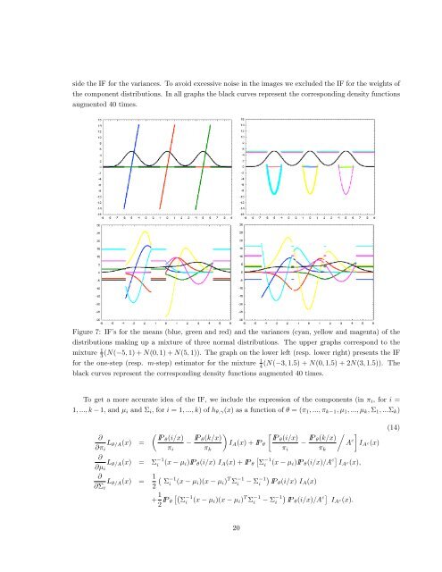
side <strong>the</strong> IF for <strong>the</strong> variances. To avoid excessive noise <strong>in</strong> <strong>the</strong> images we excluded <strong>the</strong> IF for <strong>the</strong> weights of<br />
<strong>the</strong> component distributions. In all graphs <strong>the</strong> black curves represent <strong>the</strong> correspond<strong>in</strong>g density functions<br />
augmented 40 times.<br />
Figure 7: IF’s for <strong>the</strong> means (blue, green and red) and <strong>the</strong> variances (cyan, yellow and magenta) of <strong>the</strong><br />
distributions mak<strong>in</strong>g up a <strong>mixture</strong> of three normal distributions. The upper graphs correspond to <strong>the</strong><br />
<strong>mixture</strong> 1 3<br />
(N(−5, 1) + N(0, 1) + N(5, 1)). The graph on <strong>the</strong> lower left (resp. lower right) presents <strong>the</strong> IF<br />
for <strong>the</strong> one-step (resp. m-step) estimator for <strong>the</strong> <strong>mixture</strong> 1 4<br />
(N(−3, 1.5) + N(0, 1.5) + 2N(3, 1.5)). The<br />
black curves represent <strong>the</strong> correspond<strong>in</strong>g density functions augmented 40 times.<br />
To get a more accurate idea of <strong>the</strong> IF, we <strong>in</strong>clude <strong>the</strong> expression of <strong>the</strong> components (<strong>in</strong> π i , for i =<br />
1, ..., k − 1, and µ i and Σ i , for i = 1, ..., k) of h θ,γ (x) as a function of θ = (π 1 , ..., π k−1 , µ 1 , ..., µ k , Σ 1 , ...Σ k )<br />
(<br />
∂<br />
IP θ (i/x)<br />
L θ/A (x) =<br />
∂π i π i<br />
∂<br />
L θ/A (x) = Σ −1<br />
i<br />
∂µ i<br />
∂<br />
L θ/A (x) = 1 ∂Σ i 2<br />
− IP )<br />
[<br />
θ(k/x)<br />
IP θ (i/x)<br />
I A (x) + IP θ − IP / ]<br />
θ(k/x)<br />
A c I A c(x)<br />
π k π i π k<br />
[<br />
(x − µ i )IP θ (i/x) I A (x) + IP θ Σ<br />
−1<br />
i (x − µ i )IP θ (i/x)/A c] I A c(x),<br />
(<br />
Σ<br />
−1<br />
i (x − µ i )(x − µ i ) T Σ −1<br />
i<br />
+ 1 2 IP θ<br />
[(<br />
Σ<br />
−1<br />
i (x − µ i )(x − µ i ) T Σ −1<br />
i<br />
− Σ −1 )<br />
i IP θ (i/x) I A (x)<br />
− Σ −1 )<br />
i IP θ (i/x)/A c] I A c(x).<br />
(14)<br />
20