LOCALLY STATIONARY VECTOR PROCESSES AND ADAPTIVE ...

LOCALLY STATIONARY VECTOR PROCESSES
AND ADAPTIVE MULTIVARIATE MODELING
David S. Matteson † , Nicholas A. James, William B. Nicholson and Louis C. Segalini
Cornell University
Department of Statistical Science
1198 Comstock Hall, Ithaca, NY 14853
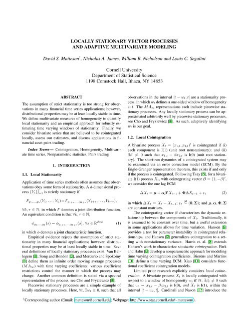
ABSTRACT
The assumption of strict stationarity is too strong for observations
in many financial time series applications; however,
distributional properties may be at least locally stable in time.
We define multivariate measures of homogeneity to quantify
local stationarity and an empirical approach for robustly estimating
time varying windows of stationarity. Finally, we
consider bivariate series that are believed to be cointegrated
locally, assess our estimates, and discuss applications in financial
asset pairs trading.
Index Terms— Cointegration, Homogeneity, Multivariate
time series, Nonparametric statistics, Pairs trading
1.1. Local Stationarity
1. INTRODUCTION
Application of time series methods often assumes that observations
obey some form of stationarity. A d-dimensional process
{Y t } T t=1 is strictly stationary if
F y1,...,y k
(Y 1 , . . . , Y k )=F y1+τ ,...,y k+τ
(Y 1+τ , . . . , Y k+τ ),
∀k, τ ∈ N, in which F denotes a joint distribution function.
An equivalent condition is that ∀k, τ ∈ N,
φ y1,...,y k
(s) = φ y1+τ ,...,y k+τ
(s), ∀s ∈ R d×k (1)
in which φ denotes a joint characteristic function.
Empirical evidence rejects the assumption of strict stationarity
in many financial applications; however, distributional
properties may be at least locally stable in time. Several
definitions of locally stationary processes exist. Van Bellegem
[1], Song and Bondon [2], and Mercurio and Spokoiny
[3] define them as infinite order moving average processes
(MA ∞ ) with time varying coefficients; various coefficient
restrictions control the manner in which the process may
change. Another common definition is stated via a spectral
representation of the process, see Cho and Fryzlewicz [4].
Piecewise stationary processes are a simple example of
locally stationary processes. Here, ∀t, ∃w t ≥ 0, such that all
observations in the interval [t − w t , t] are a stationarity process,
in which w t defines a one-sided window of homogeneity
at t. The MA ∞ representations each include piecewise stationary
processes. Any locally stationary process can be approximated
arbitrarily well by piecewise stationary processes,
see Cho and Fryzlewicz [4]. As such, adaptively identifying
w t is our goal.
1.2. Local Cointegration
A bivariate process X t = (x 1,t , x 2,t ) ′ is cointegrated if (i)
each component is I(1) (unit root nonstationary); and (ii)
∃β ≠ 0 such that x 1,t − βx 2,t is I(0) (unit root stationary).
The short-run dynamics of a cointegrated system may
be examined via an error correction model (ECM). By the
Engle-Granger representation theorem, this exists if and only
if the process is cointegrated. Following Tsay [5], for a bivariate
I(1) process X t , with cointegrating vector β = (1, −β) ′ ,
we consider the one lag ECM
∆X t = µ + αβ ′ X t−1 + Φ∆X t−1 + ε t (2)
iid
in which ∆X t = X t − X t−1 ; ε t ∼ (0, Σ); and µ, α, Φ, Σ
are constant matrices.
The cointegrating vector β characterizes the dynamic relationship
between the components of X t . Traditionally, it
is assumed to be constant over time, but a useful extension
in some applications allows for time variation. Hansen [6]
provides a test for parameter instability in cointegrated relationships,
and Hansen [7] generalizes cointegration to a setting
with nonstationary variance. Harris et. al. [8] extends
Hansen’s work to characterize stochastic cointegration. Park
and Hahn [9] develop a nonparametric approach for modeling
time varying cointegration coefficients. Bierens and Martins
[10] define a time varying ECM. Xiao [11] considers functional
coefficient cointegration models.
Limited prior research explicitly considers local cointegration.
A bivariate process X t is locally cointegrated with
respect to a window of homogeneity w t if ∀t, ∃β t ≠ 0 such
that u t = x 1,t − β t x 2,t is I(0), and X t is I(1), within the
interval [t − w t , t]. Cardinali and Nason [12] introduce the
† Corresponding author (Email: matteson@cornell.edu; Webpage: http://www.stat.cornell.edu/∼matteson/).

more general notion of costationarity. The components of X t
are costationary if there exist “deterministic, complexity constrained
sequences” {a t } and {b t } such that a t x 1,t + b t x 2,t
is a stationary process. Unfortunately, unique solutions may
not exist, and no procedure is currently available to identify
which is best.
2. MEASURING HOMOGENEITY
Let Z 1 , . . . , Z T ∈ R d be a sequence of vector observations
with E|Z t | 2 < ∞, ∀t. Let A and B denote two disjoint subsets
of {Z t }, each with contiguous observations. Matteson
and James [13] show that for independent sequences, a nonnegative
divergence measure based on characteristic functions
can be used to consistently estimate arbitrary changes in distribution.
Here, we similarly propose measuring divergence
in distribution with respect to empirical characteristic functions
ˆφ. A first order divergence measure ̂D(A, B; α) is defined
as
∫R d | ˆφ A (s) − ˆφ B (s)| 2 (
2π
d
2 Γ( 2−α
2 )
α2 α Γ( d+α
2 ) |s|d+α ) −1
ds, (3)
for some α ∈ (0, 2). We use α = 1 in Section 3.
This may easily be extended to higher orders by jointly
considering lagged values of the process. For example, a second
order measure considers two disjoint subsets of the process
{(Z t, ′ Z t−1) ′ ′ } ∈ R 2d , evaluated analogously to Equation
(3). When the observations within each subset are homogeneous,
the first order measure may be used to test Equation (1)
at a particular τ, for k = 1, while the second order measure
simultaneously considers k = 1, 2.
We apply this divergence measure to identify a window
of homogeneity at time t by first dividing the series
into K + 1 subsets, each of size δ ≥ 2, as follows: let
A = {Z t−δ+1 , . . . , Z t } and, given a strictly increasing sequence
{d i } ∈ N, let B i = {Z t−2δ+2−di , . . . , Z t−δ+1−di }.
Here, A is disjoint from each B i , but the B i may not be
disjoint. We then iteratively test for homogeneity between
subsets A and B i for i = 1, 2, ..., K, as detailed in Section
2.1. If the null hypothesis of homogeneity between
A and B i is rejected, the procedure terminates and returns
w t = max(δ, δ − 1 + d i ); otherwise, we increase to index
i + 1 and repeat.
2.1. Testing
In this section we outline a testing procedure tailored for a
bivariate series {X t } that is believed to be cointegrated locally.
We first assume that at time t the local cointegration
conditions hold for the interval [t − δ + 1, t], such that both
Z t = ∆X t and u t = x 1t − βx 2t are stationary. Here, β is
estimated using ordinary least squares (OLS) over this interval,
as discussed in Section 3. We now construct the subset A
of {Z t }, as in the previous section, and analogously construct
a subset C of {u t }. Similarly, we construct the subsets B i
of {Z t }, as well as corresponding subsets D i of {u t }. Note
that the subsets D i are based on the original estimate of β.
Finally, we define a joint test statistic as
̂D i = ̂D(A, B i ; α) + ̂D(C, D i ; α). (4)
̂D
(r)
i
The distribution of ̂D i under the dual homogeneity null
hypothesis is unknown; we propose to approximate it via simulation.
We consider the serial dependence of Z t and u t via
a VAR(1) and AR(1) model, respectively. We estimate the
mean and variance parameters for each sequence via OLS, using
the subsets A and C, respectively. Based on these parameter
estimates, we generate new sequences {Zt ∗ } and {u ∗ t },
with normally distributed errors. The series are initialized at
Zt−2δ+2−d ∗ i
= Z t−2δ+2−di and u ∗ t−2δ+2−d i
= u t−2δ+2−di .
This is repeated R times, and for the rth simulation, we calculate
= ̂D(A ∗ , Bi ∗; α) + ̂D(C ∗ , Di ∗ ; α), analogous to
Equation (4). Finally, we calculate an approximate p-value
for ̂D i as #{r : ̂D i ≤ }/R.
̂D
(r)
i
3. APPLICATION
We apply the proposed adaptive window estimation method
to potentially cointegrated stocks prices. We consider the
adjusted daily closing stock prices for Coca-Cola (KO) and
Pepsi (PEP), Hewlett-Packard (HPQ) and Dell (DELL), Wal-
Mart (WMT) and Target (TGT), and Chevron (CVX) and
Exxon Mobil (XOM). For each of these pairs we perform
analysis for the time period January 2007 through November
2012. The adjusted daily closing prices are shown in
Figures 1(a) and 2(a)(b)(c), respectively. We use δ = 30,
d i = i, R = 100 and 0.10 as the significance level for our
testing. When applied iteratively, the significance level only
corresponds to the individual marginal tests.
We used OLS to perform our procedure instead of the
maximum likelihood method of Johansen [14] due to the latter’s
irregular finite sample properties. Phillips [15] remarks
that in small samples, the maximum likelihood estimator of
the cointegrating vector has no finite moments, which can
lead to extremely large cointegration coefficients.
For each pair, we perform our estimation procedure over
each locally stationary window estimate [t − w t , t], shown in
Figures 1(b) and 2(d)(e)(f). For the KO-PEP pair, the values
of the local cointegrating coefficient ˆβ(t, w t ), an estimate
over a fixed window length ˆβ(t, ¯w = 68), as well as a cumulative
window ˆβ t with [1, t], are shown in Figure 1(c).
We perform a Dickey Fuller test to provide an additional
check that the cointegrating vector produces an I(0) process.
As stated in Zivot [16], the Dickey Fuller test examines the
cointegrated series {û t } and tests the hypotheses H 0 : û t ∼
I(1) versus H 1 : û t ∼ I(0). It should be noted since the test

(a)
(b)
Adjusted Daily Closing Stock Price
20 30 40 50 60 70
PEP
KO
Year
2007 2009 2011 2013
[t−w t ,t]
2007 2009 2011 2013
2007 2009 2011 2013
Year
Year
(c)
(d)
Cointegration Coefficient
−0.5 0.0 0.5
[t−w t,t]
[t−w,t]
[1,t]
Dickey Fuller Test Statistic
−4 −3 −2 −1 0 1
Test Statistic
10% C.V.
5% C.V.
1% C.V.
2007 2009 2011 2013
2007 2009 2011 2013
Year
Year
Fig. 1. (a) The Pepsi (PEP) and Coca-Cola (KO) adjusted daily closing stock prices for January 2007 through November 2012;
(b) [t − w t , t], our estimated window of local stationarity at times t; (c) estimated local cointegrating coefficient ˆβ(t, w t ) over
locally stationary windows [t − w t , t], ˆβ(t, ¯w), estimated over a fixed width window [t − ¯w, t] using width 68, the mean of
w t , and ˆβ t , the cointegrating coefficient using all available data up to time t; (d) Dickey-Fuller test statistic over each locally
stationary window, along with 1, 5, and 10 percent critical values, which are used to confirm whether the cointegrated process
is unit root stationary over each interval [t − w t , t].
is residual based, the distribution of the test statistic is nonstandard
and follows a “Dickey Fuller Table.” Figure 1(d)
shows the Dickey-Fuller test statistic for the KO-PEP series,
along with the 10, 5, and 1 percent critical values. Since large
negative values provide evidence for rejection of H 0 , the test
implies that {û t } has extended periods of local stationarity.
3.1. Pairs trading
Pairs trading is a strategy that was developed in the 1980s at
Morgan Stanley, and elsewhere. It involves selecting a pair of
stocks that have correlated prices, then buying the relatively
cheaper stock, while shorting the relatively expensive stock.
The positions are entered when the prices have diverged and
exited once the prices converge.
Although correlated stock prices indicate a linear association
over time, there is no guarantee divergent prices will necessarily
converge. However, the relative prices, or the spread
u t , for pairs that are cointegrated will have an equilibrium;
mean reversion of u t may be used to improve trading decisions.
Several authors have proposed various execution criteria.
Dunis et al. [17] open a position when the spread has diverged
from its historical mean by two historical standard deviations.
They exit once the spread has returned to within half of one
standard deviation from the mean. Gatev et al. [18] use a
similar approach. Historical backtesting is conducted to justify
the two standard deviation rule. To rely less on historical
data, Ehrman [19] proposes normalizing the pair’s divergence
by taking the absolute pair difference, subtracting
the 10-day moving average and then dividing by the 10-day
standard deviation. Alternatively, the relative strength index,
which indicates oversold and overbought conditions, is applied
in Ehrman [19].
Any of the above strategies may be implemented using
the proposed adaptive window of homogeneity index w t . For
example, at time t we may implement a standard deviation
rule using û t = ̂mean(u s : s ∈ [t − w t , t]) and ˆσ 2 t = ̂var(u s :
s ∈ [t − w t , t]). Define a normalized process
ũ s = u s − û t
ˆσ t
for s ∈ [t − w t + 1, t + δ].

(a)
(b)
(c)
Adjusted Daily Closing Stock Price
30 40 50 60 70
WMT
TGT
Adjusted Daily Closing Stock Price
10 20 30 40 50
HPQ
DELL
Adjusted Daily Closing Stock Price
50 60 70 80 90 100 110
XOM
CVX
2007 2009 2011 2013
2007 2009 2011 2013
2007 2009 2011 2013
Year
Year
Year
(d)
(e)
(f)
Year
2007 2009 2011 2013
[t−wt,t]
Year
2007 2009 2011 2013
[t−wt,t]
Year
2007 2009 2011 2013
[t−wt,t]
2007 2009 2011 2013
2007 2009 2011 2013
2007 2009 2011 2013
Year
Year
Year
Fig. 2. (a),(b),(c) The adjusted daily closing prices from January 2007 through November 2012 of Walmart (WMT) & Target
(TGT), Hewlett Packard (HPQ) & Dell (DELL), and Exxon Mobil (XOM) & Chevron (CVX), respectively; (d),(e),(f) the
estimated window of local stationarity [t − w t , t], at times t, for WMT & TGT, HPQ & DELL, and XOM & CVX, respectively.
Then, we may enter a position if |ũ t | > 2, and exit at s >
t once |ũ s | < 0.5, |ũ s | > 3, or s = t + δ, whichever is
sooner. This strategy may similarly be implemented using a
fixed width window [t − ¯w, t] or a cumulative window [1, t],
for comparison.
First, for the KO-PEP series we compare the results of
this trading strategy for the three window methods. The first
70 observations are used for initialization, and we use δ =
30. For a fixed width window, ¯w = 68, we entered a trading
position on 14.7% of the 1450 days; the mean return per trade
was -7% and the mean return per day was -3%. Using the
cumulative window [1, t], we entered a position on 26.8% of
the days; the mean return per trade was 12% and the mean
return per day was -2%. Finally, when using the adaptively
estimated window [t − w t , t] via the proposed approach we
entered a trading position on 15.7% of the days; the mean
return per trade was 21% and the mean return per day was 2%.
Positions were held a mean of 7.8 days using the adaptive and
fixed window approaches, and 16.9 days using the cumulative
window.
When applied to the other pairs, similar results were obtained.
For these cases, the proposed adaptive window approach
resulted in a higher mean return per trade than when
using either a fixed or cumulative window, see Table 1. The
mean trade durations in days are shown in Table 2. In most
cases, these higher mean returns were obtained while holding
positions for shorter periods.
Mean Return (per trade)
Window/Pair KO-PEP HPQ-DELL WMT-TGT XOM-CVX
Fixed -7.0% 2.5% -6.6% 0.9%
Cumulative 12.0% -0.9% -0.1% -1.8%
Adaptive 21.0% 4.4% 1.1% 43.0%
Table 1. The mean return (per trade) for the three window
methods on the selected pairs.
Mean Trade Duration (days)
Window/Pair KO-PEP HPQ-DELL WMT-TGT XOM-CVX
Fixed 7.8 9.7 9.7 8.5
Cumulative 16.9 23.0 13.4 17.8
Adaptive 7.8 8.2 8.3 10.6
Table 2. The mean trade duration (days) for the three window
methods on the selected pairs.
4. CONCLUSION
We have proposed a novel method for estimating a window
of homogeneity and extended this approach for adaptively
estimating a window of local cointegration. We apply this
approach to a simple pairs trading strategy and find that an
adaptive window outperforms fixed and cumulative windows,
for the data considered. The realized returns are complexly
related and approximate risk adjustment requires additional
consideration; further analysis is necessary to fully assess the
suitability of this approach for pairs trading in general.

5. REFERENCES
[1] Van Bellegem, S., “Locally stationary volatility modelling,”
in Handbook of Volatility Models and Their Applications,
2011.
[2] Song, L. and Bondon, P., “A local stationary longmemory
model for internet traffic,” in 17th European Signal
Processing Conference, 2009.
[3] Mercurio, D. and Spokoiny, V., “Statistical inference for
time-inhomogeneous volatility models,” Annals of Statistics,
vol. 32, no. 2, pp. 577 – 602, 2004.
[4] Cho, H. and Fryzlewicz, P., “Multiscale breakpoint detection
in piecewise stationary AR models,” in 4th World
Conference of the IASC, 2008.
[16] Zivot, E. and Wang, J., Modeling financial time series
with S-PLUS, Springer Verlag, 2006.
[17] Dunis, C.L., Giorgioni, G., Laws, J. and Rudy, J., “Statistical
arbitrage and high-frequency data with an application
to Eurostoxx 50 equities,” Liverpool Business School,
Working paper, 2010.
[18] Gatev, E., Goetzmann, W.N. and Rouwenhorst, K.G.,
“Pairs trading: Performance of a relative-value arbitrage
rule,” Review of Financial Studies, vol. 19, no. 3, pp. 797–
827, 2006.
[19] Ehrman, D.S., The handbook of pairs trading: Strategies
using equities, options, and futures, Wiley, 2006.
[5] Tsay, R.S., Analysis of Financial Time Series, Wiley,
2010.
[6] Hansen, B.E., “Tests for parameter instability in regressions
with I(1) processes,” Journal of Business & Economic
Statistics, vol. 20, no. 1, pp. 45–59, 1992.
[7] Hansen, B.E., “Heteroskedastic cointegration,” Journal
of Econometrics, vol. 54, no. 1, pp. 139–158, 1992.
[8] Harris, D., McCabe, B. and Leybourne, S., “Stochastic
cointegration: estimation and inference,” Journal of
Econometrics, vol. 111, no. 2, pp. 363–384, 2002.
[9] Park, J.Y. and Hahn, S.B., “Cointegrating regressions
with time varying coefficients,” Econometric Theory, vol.
15, no. 5, pp. 664–703, 1999.
[10] Bierens, H.J. and Martins, L.F., “Time varying cointegration,”
Econometric Theory, vol. 26, no. 05, pp. 1453–
1490, 2010.
[11] Xiao, Z., “Functional coefficient cointegration models,”
Journal of Econometrics, vol. 152, no. 2, pp. 81–92, 2009.
[12] Cardinali, A. and Nason, G.P., “Costationarity of locally
stationary time series,” Journal of Time Series Econometrics,
vol. 2, no. 2, 2010.
[13] Matteson, D.S. and James, N.A., “A nonparametric approach
for multiple change point analysis of multivariate
data,” under review, 2012.
[14] Johansen, S., Likelihood-based inference in cointegrated
vector autoregressive models, Cambridge University
Press, 1995.
[15] Phillips, P.C.B., “Some exact distribution theory for
maximum likelihood estimators of cointegrating coefficients
in error correction models,” Econometrica, vol. 62,
no. 1, pp. 73–93, 1994.