Download - ASLO

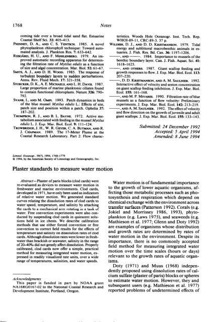
1768 Notes
coming tide over a broad tidal sand flat. Estuarine
Coastal Shelf Sci. 32: 4054 13.
PHINNEY, D. A., AND C. S. YENTSCH. 1985. A novel
phytoplankton chlorophyll technique: Toward automated
analysis. J. Plankton Res. 7: 633-642.
RIISGARD, H. U., AND F. MBHLENBERG. 1979. An improved
automatic recording apparatus for determining
the filtration rate of MytiZus edulis as a function
of size and algal concentration. Mar. Biol. 52: 6 l-67.
SMITS, A. J., AND D. H. WOOD. 1985. The response of
turbulent boundary layers to sudden perturbations.
Annu. Rev. Fluid Mech. 17: 321-358.
STOECKER, D. K., A. E. MICHAELS, AND L. H. DAVIS. 1987.
Large proportion of marine planktonic ciliates found
to contain functional chloroplasts. Nature 326: 79&
792.
SVANE, I., AND M. OMPI. 1993. Patch dynamics in beds
of the blue mussel MytiZus edulis L.: Effects of site,
patch size and position within a patch. Ophelia 37:
187-202.
THOMPSON, R. J., AND B. L. BAYNE. 1972. Active metabolism
associated with feeding in the mussel A4ytiZu.s
edulis L. J. Exp. Mar. Biol. Ecol. 9: 111-124.
TROWBRIDGE, J. H., W. R. GEYER, C. A. BuT)~~AN, AND R.
J. -MAN. 1989. The 17-Meter Flume at the
Coastal Research Laboratory. Part 2: Flow charac-
teristics. Woods Hole Oceanogr. Inst. Tech. Rep.
WHOI-89-1 1, CRC-89-3. 37 p.
WILDISH, D. J., AND D. D. KRISTMANSON. 1979. Tidal
energy and sublittoral macrobenthic animals in estuaries.
J. Fish. Res. Bd. Can. 36: 1197-1206.
- 1984. Importance to mussels of the
bend boundary layer. Can. J. Fish. Aquat. Sci. 41:
1618-1625.
- AND OTHERS. 1987. Giant scallop feeding and
growth responses to flow. J. Exp. Mar. Biol. Ecol. 113:
207-220.
-, D. D. KRISTMANSON, AND A. M. SAULNIER. 1992.
Interactive effect of velocity and seston concentration
on giant scallop feeding inhibition. J. Exp. Mar. Biol.
Ecol. 155: 161-168.
-, AND M. P. MIYARES. 1990. Filtration rate of blue
mussels as a function of flow velocity: Preliminary
experiments. J. Exp. Mar. Biol. Ecol. 142: 213-219.
-, AND A. M. SAULNIER. 1992. The effect ofvelocity
and flow direction on the growth ofjuvenile and adult
giant scallops. J. Exp. Mar. Biol. Ecol. 155: 133-143.
Submitted: 24 December 1992
Accepted: 5 April 1994
Amended: 8 June 1994
Limnol. Oceanogr., 39(7), 1994, 1768-1779
Q 1994, by the American society of Limnology and -w-why, Inc.
Plaster standards to measure water motion
Abstract-Plaster of paris blocks (clod cards) were
re-evaluated as devices to measure water motion in
freshwater and marine environments. Clod cards,
developed in 1971, have only been used as indicators
of relative water motion. We generated standard
curves relating the dissolution rates of clod cards to
water speed, temperature, and salinity by attaching
the cards to a mechanical arm rotating in a tank of
water. Free convection experiments were also conducted
by suspending clod cards in quiescent solutions
held in ice chests. We describe calibration
methods that use either forced convection or free
convection to correct field results for the effects of
temperature and salinity on dissolution rates of clod
cards. Although dissolution rates were lower in freshwater
than brackish or seawater, salinity in the range
of 20-4wm did not greatly affect dissolution. Properly
calibrated, clod cards now offer a simple, practical
method for measuring integrated water motion, expressed
in readily visualized rate units, over a wide
range of temperatures, salinities, and water speeds.
Water motion is of fundamental importance
to the growth of lower aquatic organisms, affecting
those metabolic processes such as photosynthesis
and respiration which depend on
chemical exchange with the environment across
transfer surfaces (Patterson 1992). Corals (e.g.
Jokiel and Morrissey 1986, 1993), phytoplankton
(e.g. Laws 1975), and seaweeds (e.g.
Mathieson et al. 1977; Glenn and Doty 1992)
are examples of organisms whose distribution
and growth rates are determined by rates of
water motion in the environment. Despite its
importance, there is no commonly accepted
field method for measuring integrated water
motion over the time scales (hours or days)
relevant to the growth rates of aquatic organisms.
Doty (197 1) and Muus (1968) independently
proposed using dissolution rates of calcium
sulfate (plaster of paris) blocks or spheres
to estimate water motion. However, they and
subsequent users (e.g. Mathieson et al. 1977)
reported problems of undetermined effects of

Notes 1769
salinity and temperature on results. Nevertheless,
the clod cards proposed by Doty are easily
prepared with standard ice-cube trays as molds
and are suited to marine studies because they
are large enough to be left out through a tide
cycle without dissolving completely. It is a
convenient and inexpensive method of measuring
water motion in field studies. We have
attempted to define the behavior of clod cards
with respect to temperature and salinity and
to develop calibration methods to enhance their
usefulness.
In his original description, Doty (197 1) recommended
expressing field results as a “diffusion
increase factor” (DF), defined as the
ratio of weight loss of clod cards placed in the
field to the weight loss of clod cards from the
same batch held under specified still-water
conditions in the laboratory. DF was meant to
express the multiplication factor of diffusion
in the field relative to diffusion in the absence
of water motion. Unfortunately, his reported
still-water values sometimes varied inexplicably
among batches of clod cards that had
been prepared and measured the same way.
This variation introduced a large potential error
into the calculation of DF, since this relatively
small number is used as a divisor.
Doty’s laboratory calibration method consisted
of placing five clod cards on the bottom
of a 15-cm-diameter container to which 2 liters
of test solution were added. The water (motionless)
was changed every day for 4 d. The
initial and final dry weights of the clod cards
were used in the DF calculations. Howerton
and Boyd (1992) as well as Jokiel and Morrissey
(1993) have demonstrated that the calibration
container must have a minimum volume
of 20 liters per clod card if it is to accurately
represent weight loss due to diffusion in totally
calm water.
An additional problem is created by stratification
in the calibration container, particu-
larly when the clod cards are placed on the
bottom. When a solid dissolves in quiescent
water, material from the solid dissolves and
diffuses away from the surface, producing a
solution near the solid that is denser than the
water itself. This solution flows downward, and
the resulting flow increases the dissolution rate.
However, the dense solution may “pool” on
the bottom of the container, creating a layer
of solution with a higher concentration of the
dissolving material than in the bulk liquid. If
the dissolving solid is placed on the bottom of
the container, it will generate a layer of relatively
concentrated liquid that will retard the
dissolution rate compared to the solid in pure
bulk solution.
In unpublished experiments pointing the way
to an improvement in methodology, Doty attached
clod cards to a rotating arm in a tank
of seawater and found that the dissolution rates
of the cards were proportional to the rate at
which they moved through the water. He called
the apparatus a “water motion simulator”
(WAMOSI) because it was the clod card, not
the water, that was moving. The raw data tabulation
of that study (Doty et al. 1986) shows
that despite differences in apparent still-water
dissolution rates among different batches of
clod cards, their actual dissolution rates on the
rotating arm were reproducible at a given velocity.
Subsequently, Glenn and Doty (1992)
used the rotating-arm calibration method in
combination with field measurements to show
that 85-98% of the variability of growth rates
of eucheumatoid red seaweeds across seasons
on a reef flat in Hawaii could be explained by
water motion. These experiments indicated
that calibrated clod cards would be valuable
tools for correlating growth rates with water
motion in the marine environment.
Recently, Howerton and Boyd (1992) used
clod cards to measure circulation patterns in
aquaculture ponds, and Jokiel and Morrissey
(1993) used clod cards to study water motion
on coral reefs. In both studies, the investigators
improved the still-water calibration method
by increasing the volume of water into which
the cards dissolve, and they measured rates of
still-water dissolution of the cards as functions
of duration of exposure, temperature, and salinity.
Both studies used a rotating arm to estimate
dissolution rates as a function of water
velocity at a single temperature and salinity.
They concluded that clod cards were valuable
in measuring relative rates of water motion
but, similar to earlier investigators, cited the
need for equations relating card dissolution
rates to fluid velocity as influenced by temperature
and salinity before they could be used
to measure absolute water velocities. Deriving
and validating these equations was the purpose
of our study.
Clod cards were prepared essentially ac-

1770 Notes
r=0.15
(typ.)
‘F q-
El
_
I
/‘ ‘\,
+45cm+
/F$2+.,
\
3.3cm
T=T
Bottom surface sanded
to adjust weight
to 30 f 1.5 g
Fig. 1. Dimensions of the clod cards.
cording to the methods of Doty (197 1) and
Howerton and Boyd (1992), except that neither
the starting plaster of paris nor the finished
cards were oven-dried before use. Our clod
cards were made from reagent-grade plaster of
paris (calcium sulfate hemihydrate, EM Science
Co.) with 335 ml of water per 500 g. We
slowly added plaster of paris to the water
as we stirred it with a spoon; we poured the
slurry into flexible plastic ice-cube trays and
allowed it to harden for 20-30 min before removing
the clod cards. We tapped the trays
vigorously several times while the mixture was
still liquid to dislodge air bubbles. Sometimes,
a thin layer of liquid covered the surface of the
hardening clod cards in the trays. This layer
was decanted before the cards were removed.
After removal, the cards were dried for 3 d or
longer on a laboratory bench, and the bottoms
were sanded until the cards had uniform weight
within a batch (within 1.5 g); they were then
glued to 5- x 7-cm sheets of waterproof plastic
(Nalgene PolyPaper) with silicone cement.
Weight loss due to water exposure was quantified
by weighing dry clod cards before exposure,
placing them in the test solution for
24 h, allowing them to redry for 3 d or longer
on a laboratory bench, and then reweighing
them.
The ice-cube trays used in these experiments
produced clod cards of shape and dimensions
shown in Fig. 1. Internally, the dry cards had
a foam structure with numerous interconnected
minute air spaces within the calcium sulfate
matrix. The cards had densities of 1.19-l .21
/
at 25°C and weighed 28-32 g each. When placed
in test solutions, the cards were fully saturated
within 5 min, absorbing from 10 to 12 ml of
solution.
Water motion experiments were carried out
inside a greenhouse in a shallow, wooden-sided,
square tank (2.1 m long, 0.36 m deep) with
a plastic liner (Fig. 2). The tank was filled with
test solution to a depth of 25 cm (solution
volume, 1.1 m3) and covered with sheets of
Styrofoam to control temperature during each
24-h run. Test solutions were chilled by circulating
the water through a 124-W refrigeration
unit with external thermostat by means
of a 30-W circulation pump. Solutions were
heated with a thermostat-controlled, 150-W
immersion heater.
Clod cards were attached at various positions
along a 2-m stainless steel arm (1 cm
thick) which was rotated in the tank at 2.4 rpm
by a 37-W electric gear motor secured over the
middle of the tank by an external wooden
framework. The cards were mounted on the
arm by attaching them with rubber bands to
rigid PVC-plastic plates (5 x 7.5 cm, 0.3 cm
thick) screwed to the arm. Five cards were
mounted along each of the two radii at distances
from the center of 7, 27,47,67, and 87
cm. Thus, each position was represented by
duplicate cards moving through the water at
nominal velocities ranging from 1.8 to 2 1.8
cm s-l, which are within the range of water
velocities encountered on tropical reef flats
(Glenn and Doty 1992) but lower than extreme
tidal bores, which are up to 80 cm s-l (Mathieson
et al. 1977). Greater velocities can be
achieved by selecting a gear motor with a higher
rotation rate (Howerton and Boyd 1992) or
by using a longer rotating arm (Jokiel and Morrissey
1993).
Dissolution rates under free convection conditions
were determined by suspending clod
cards by wires 5 cm below the surface of 60
liters of solution contained in ice chests. The
ice chests were kept under constant temperature
in an undisturbed indoor location during
each 4-6-d run. The cards were withdrawn and
weighed wet each day, then replaced in the
chests.
Three solutions were tested in the water motion
tank: tapwater, brackish water, and seawater.
Tapwater was from the Tucson municipal
supply, and seawater was collected from

Notes 1771
T
2.1 m
mounted
arm
mounte~~~~a level
k- 2.1 m 4
Fig. 2. Design of the water motion simulator.
a seaside well in the upper Gulf of California
at Puerto Pefiasco, Sonora, Mexico. Brackish
water was a 1 : 1 mixture of tapwater and seawater.
Salinities by refractometer were 0, 20,
and 407~. Solutions were measured for temperature,
pH, and electrical conductivity at the
start and finish of each run. Samples of each
solution were analyzed for cations and anions,
including calcium and sulfate, by AOAC
methods (Laboratory Consultants, Tempe, Ar-
Table 1. Analyses of tapwater, brackish water, and seawater
used in clod card calibration experiments.
Constituent
Tapwater 20%3 40%
Calcium 1.46 7.06 13.20
Sulfate 0.85 16.66 33.94
Boron 0.008 * 0.473
Magnesium 0.417 * 61.6
Sodium 2.13 * 534.8
Chloride 1.71 * 630.4
Fluoride 0.056 * 0.078
PH 8.1-8.5 8.1-8.2 8.2-8.3
EC (mmhos cm-‘) 715 34,000 71,500
* Brackish water (20%~) was a I : 1 mixture of tapwater and 40% water. Analyses
of elements of limited importance to this study were omitted for this
mixture.
(mol
m-l)
izona, and the Soil and Water Testing Laboratory,
University of Arizona, Tucson) (Table
1). Solutions in the tank were changed after 2-
3 runs of clod cards to reduce accumulation
of calcium sulfate in the water. The ice-chest
experiments used an additional solution, 25o/oo
salinity, also prepared by dilution of tapwater
and seawater.
Weight loss of clod cards vs. water motion
is expected to be a decreasing rather than a
linear function, because the exposed area of
the clod diminishes as dissolution proceeds.
The rate of dissolution of a solid in an aqueous
solution can be expressed as
dW
- = -kAAC.
d6
W is the weight of the solid, 8 is time, k the
mass transfer coefficient, A the exposed area
of the solid, and AC the concentration difference
between the dissolved solid in the liquid
at the solid-fluid interface and in the bulk liquid.
The dissolution of solids, including the diffusion
process across boundary layers, is described
in detail in several mass transfer texts

1772
Notes
J
1.0
2
E 0.9
L
2 0.6
P
< 0.7
t 0.6
0.010
1 10 100
Velocity, cm s-1
Fig. 3. Plot ofclod card weight loss vs. velocity through
32o/oo seawater for data from Glenn and Doty (1992) used
in the form of Eq. 3 (their data extend to higher velocities
than our work). The slope of the regression line is
0.838kO.042.
0.5
0.4 r I
0 5 10 15 20 25 30
Temperature, "C
Fig. 4. Correction factor for clod card data with T,, =
298°K and pref = viscosity of pure water at 25°C. The four
lines correspond to salinities of 0, 10, 20, and 40%~ from
top to bottom. Calculated with viscosity data from Riley
and Skit-row (1975).
(e.g., Cussler 1984; Sherwood et al. 1975; Skelland
1974). For solids of sample geometries
which dissolve uniformly, the area and weight
relationship can be approximated as
A (2)
Ai and Wi represent the initial area (exposed)
and weight of the solid. For clod cards, this
approximation is useful until > 50% of the clod
has dissolved or longer, depending on the velocity
of the fluid.
The mass transfer coefficient is also influenced
by the change in clod dimensions; however,
the effect is usually minor until well into
the dissolution process. Equations 1 and 2 can
be combined and integrated to give
1 - (?r = ;k($A,. (3)
Wr is the final weight of the clod after time 8
has elapsed. Equations 3 is useful for data analysis;
the mass transfer coefficient usually varies
with the fluid velocity raised to a power (P),
so a log-log plot of [l - (WJ/ Wi)“] against
velocity should yield a straight line. This is
illustrated in Fig. 3 with the data of Glenn and
Doty (1992). Equation 3 can be rearranged to
give an expression for the overall fraction of
weight 10~s (A W/ Wi):
Assuming that AC remained constant during
dissolution, experimental data at a given temperature
and salinity were correlated with the
model
( )
l/3
Wf = aVm.
I- j7
I
The constants a and m can be determined experimentally
by means of the rotating arm, and
weight loss data from clod cards exposed in
the field can then be used in Eq. 5 to determine
water motion.
The effect of temperature at a given salinity
and CaSO, concentration was corrected by using
the group (T/T,,) (p,.,&) to normalize data
to a reference temperature, where Tis absolute
temperature, and p is viscosity. This group (Fig.
4) is typically used to estimate the changes in
diffusion coefficients (Reid and Sherwood
1966) with varying solution strength.
From Eq. 1 and 3, the dissolution rates are
also dependent on the concentration of CaSO,
in the bulk water and factors influencing the
concentration, such as the ionic strength of the
bulk water. To determine the concentration
difference, we assume the solution at the gypsum-water
interface is saturated with CaSO,
and determine AC with the solubility product
as
Ksp = [Ca2+]i[S042-]i
g= 1 - 11 - ;k($)ACO13. (4)
or
= ([Ca’+], + AC)([S042-]b + AC) (6)

Notes
1773
0.022
30
0.020
i b 0.019
c -
5 0.016
E
- 0.017
2
0.016
I
0.015
25
I
2 20
0
c g 15
8
2
10
5
Corrected Velocity _
0.014
u 5 10 15 20 25 30 35 40
Salinity, 20
0 A
0
30 40 50 60
Rodius. cm
Fig. 5. Calculated concentration difference of CaSO,
between the solid-liquid interface and bulk solution of
clod cards in natural seawater sources based on Eq. 7.
Curve A was calculated based on literature values of seawater
chemical content at 32%1 and assuming that seawater
was diluted with distilled water to achieve the lower salinities;
curve B was calculated based on chemical analyses
of Puerto Peiiasco seawater at 40?&0 and Tucson tapwater
used as the diluent in our study.
Ac =
1(
_
[Ca2+lb + W42% 2 + K Oo5
2 1
SP
I
Ka2+lb + W42- lb
2 ) . (7)
[Ca2+]i, [Ca2+lb, [S042-]i, and [S042-]b are calcium
and sulfate ion concentrations at the interface
and in the bulk solution. Ksp is the solubility
product, which can be computed by the
expressions given by Marshall and Slusher
(1968), who allow for the presence of ion pairs
such as MgS040 in their correlations.
The values of [Ca2+16 and [S042-]b used in
Eq. 7 are based on the total calcium and sulfate
measured in solution; we have made no attempt
to correct these concentrations for the
presence of ion pairs containing calcium or
sulfate. Increasing the ionic strength (or salinity)
increases the CaSO, solubility product,
thereby increasing the gradient between the interface
and the bulk solution and accelerating
the dissolution rate of a clod card. However,
this effect is counteracted if the concentration
of CaSO, in the bulk solution increases with
salinity, which is the case with seawater; the
seawater used in our experiments contained
CaSO, at concentrations more than eight times
that of the freshwater supply. The brackish
supply, prepared by dilution, was intermediate.
Figure 5 contains salinity correction curves
Fig. 6. Correction for the induced-water-motion effect
of the rotating arm in the tank. Top line is the velocity of
the clod card in the tank at each position on the arm;
bottom line is the velocity of the water in the tank estimated
by the movement of suspended particles in the
water; middle line is the corrected velocity used to correlate
the card dissolution rates with water motion.
based on Puerto Peiiasco seawater and Tucson
tapwater used in our study (curve B) and on
literature values of normal seawater constituents
(Hansson 1973) assumed to be diluted
with distilled water (curve A). Curve B falls
below curve A because Tucson tapwater and
Puerto Pefiasco seawater contain proportionally
more CaSO, than distilled water and standard
seawater.
The water motion tank was used to obtain
data for velocity-weight loss correlations. The
velocity of the clod card through the water was
easily calculated from the rotation rate of the
arm and the distance of the card from the center
of rotation. However, it was necessary to
correct for the rotary movement imparted to
the water in the tank by the moving arm. This
movement was determined at each of the five
positions by measuring the movement of small
suspended particles in the water. A drag model
was correlated to the data and used to correct
the velocities of the cards into estimates of
their velocities relative to the water at each
position (Fig. 6). The correction was more significant
at low than at high velocities.
Forced convection tests were run at temperatures
from 13 to 35°C in three different
salinities on the rotating arm (Fig. 7). Plots in
the form of Eq. 5 were subjected to regression
analyses (Table 2). In all runs, clod card weight
loss at the lowest test velocity was increased
by free convection, and the points fell - 15%
above the curve of best fit to the other points;

1774 Notes
0.6
A 25.5’
A 30.5.
0 33.5.
Table 2. Regression analyses of clod card runs at various
salinities and temperatures. The model equation was
in the form [ 1 - (WI W,)]” = a I/‘“; both sides of the equation
were converted to natural logarithms to reduce the
equation to a linear function for analysis.
a
0 2 4 6 6
Velocity. cm a-l
14 16
20
0 13.0 8 0.0146 0.653 0.992 3.16
0 19.5 8 0.0126 0.749 0.992 3.67
0 25.5 8 0.0157 0.772 0.997 2.49
0 30.5 8 0.0178 0.750 0.984 5.33
0 33.5 8 0.0187 0.799 0.996 2.81
20 12.0 8 0.0141 0.765 0.988 4.73
20 19.0 8 0.0136 0.823 0.991 4.43
20 25.5 8 0.0164 0.867 0.990 4.75
20 30.7 8 0.0180 0.868 0.997 2.95
40 13.0 8 0.0130 0.768 0.994 3.24
40 24.5 8 0.0183 0.793 0.998 2.53
40 28.3 8 0.0307 0.757 0.987 4.84
Temperature compensated
0 40 0.0162
20 32 0.0176
40 24 0.0204
0.745 0.965 6.94
0.83 1 0.976 6.41
0.773 0.984 4.93
0.6
V.”
0 2 4 6 6 10 12 14 16 16 20
Velocity, cm *-l
0 13% (4O.h.) C
0 2 4 6 6 10 12 14 16 16 20
Velocity, cm se1
Fig. 7. Temperature curves for clod cards run at different
velocities in tapwater (A), brackish water (B), and
seawater (C). Lines were fit to data points using Eq. 5.
hence, data for the lowest velocity were omitted
from curve fitting. The model equation can
be used to calculate V as long as the velocity
is >2 cm s-l.
Coefficients of determination (r2) were 0.98
or higher, and percent error of estimates of y
were in the range 2.5-6.0%. Although m varied
somewhat, the mean value was -0.8, the value
expected for mass transfer from a flat surface
in a turbulent flow (Skelland 1974). As expected,
increased temperatures accelerated the
dissolution rates of clod cards at all test salin-
ities. For the temperature-compensated sequence
of Table 2, [ 1 - ( Wr/ Wi)“] was divided
by (T/T,,,) (P,&). Note that temperature-corrected
data fell onto a response surface of the
shape predicted by calculations of AC (Fig. 8).
The effects of both temperature and salinity
variations are included in the experimental data
correlation (Eq. 8). Dissolution rates were lower
in tapwater than in brackish water or seawater
at a given temperature, but over the range
20-40?& salinity had a minor effect on dissolution
rates. Hence, salinity does not appear
to be a major factor controlling dissolution
rates in marine systems.
The dimensional equation fitting our data is
%=I -[I -0.71(~)($-Jy)
(8)
with Y = 0.985. The concemration difference,
AC,, (mol liter-‘), is computed at 25°C by
means of Eq. 7 or Fig. 4; 8 is expressed in days
and V in cm s-l. The average ratio of Ai : Wi
for our clod cards was 1.38 cm2 g- l.
The results of mass transfer experiments are
commonly reported in terms of the appropriate
dimensionless groups, although most readers
will likely find equations such as Eq. 8 more

Notes 1775
Note: Data adjusted to 25%
Fig. 8. Temperature-corrected data for clod cards run at different velocities in tapwater (O?%O), brackish water (20%0),
and seawater (40%0). The data points are superimposed on a response surface based on Eq. 4 with k proportional to
W.s and with AC calculated from Eq. 7 for Puerto Peiiasco seawater. Note that experimental data points fall on the
response surface except at lowest velocity where free convection affects dissolution rates of the cards.
convenient for use with marine systems since
all the information required can usually be obtained
from Figs. 4 and 5. Our forced convection
data can also be described by the expression
NSh = 0 . 059NgtN SC N - (9)
Ns,, is the Sherwood number (kLID,), NRe the
Reynolds number (L VP/~), and Nsc the Schmidt
number (p/pDJ In the dimensionless groups,
k is the mass transfer coefficient evaluated with
Eq. 3 (with AC evaluated at solution temperature
and salinity), D, the volumetric molecular
difhtsion coefficient, p the viscosity, p the
liquid density, and L a geometry term determined
by the shape and orientation of the object.
The geometry term introduced by Pasternak
and Gauvin (1960) was used, where L
= (surface area of body) + (perimeter of projected
area perpendicular to flow). The mounting
card was included in the calculation of the
geometry term. The average value of L in these
studies was 5.4 cm.
Fluid properties were evaluated based on the
bulk solution, with density and viscosity data
from Riley and Skirrow ( 197 5). Diffusion co-
efficients were calculated from equations given
by Cussler (1984), Perry and Chilton (1973),
and Dickson and Whitfield (198 1). Despite the
large amount of information in the literature
on scale formation in seawater, no experimental
values for CaSO, diffusion coefficients in
seawater could be located to compare with the
computed values. At 25”C, the spread in the
values of the difhtsion coefficients for the different
salinities was on the order of 5%.
Figure 9 compares our clod card data and
those of Glenn and Doty (1992) with equations
for spheres and flat plates. Glenn and Doty did
not include a number of details relating to their
clod cards and calibration conditions (e.g. block
dimensions, water temperature, and salinity),
so we did not use their data in obtaining Eq.
9. With respect to other geometries, the clod
card data are roughly the same magnitude as
predicted by the sphere equation (Pasternak
and Gauvin 1960), but the slope is different,
possibly due to the presence of the mounting
card. The flat-plate equation (Skelland 1974)
parallels the clod card data but is substantially
lower.
Both Doty (197 1) and Muus (1968) expe-

1776
Notes
1000
500
< 200
p 100
7
f 50
3 Tap. ’
v 20 30
0 32 30
b 40 “/.o
0.5
e- 0.4
B
z- 0.3
P
E
6
z
0.2
0 Baker (Tap, 30.3YZ)
A EMS (Tap, 30.5’C)
20
f 0.1
10
200 500 1000 2000 5000 lE4 2E4 5E4 lE5
Fig. 9. Comparison of clod card data with the equation
of Pastemak and Gauvin (1960) for spheres (dashed line)
and the equation for a flat plate (Skelland 1974), represented
by the dotted line. The data of Glenn and Doty
(1992) for 32960 seawater are shown, but were not used in
obtaining Eq. 12. The points below iVRe = 1,000 are increased
by natural convection and were also omitted from
the correlation.
NRI?
rienced problems of variability of weight loss
under uniform conditions by clod cards from
the same batch. Referring to Fig. 2, the variability
of clod card weight loss in our tests can
be estimated by comparing the loss from
matched pairs of cards at the same radial position
on the arm (1, 2, 3, . . .) but on opposite
sides of the arm. For all of our runs with
EM Science plaster of paris at the different temperatures,
salinities, and speeds, the standard
deviation of the weight loss differences, as
[CA w/KLIe* - (A IV/ WJsideZ], was 0.0135,
while the overall average difference was 7.7 x
10m4 (n = 60), which is not significantly different
from zero (P = 0.05). Extreme variability
of weight loss within a batch of cards
caused no problems during our tests.
We also ran limited tests with plaster of paris
from Sargent-Welsh Chemical Co. (technical
grade) and from Baker Scientific Co. (reagent,
extra-fine powder ~44 pm, suitable for electrophoresis
gel). The Sargent-Welsh material
produced clod cards of the same density as the
EM Science material used throughout these
tests; a slight excess of water (375 ml : 500 g)
used with the Sargent-Welsh plaster also failed
to alter the final density. There was no significant
difference between the dissolution rates
of cards made with the Sargent-Welsh plaster
and those made with EM Science material when
tested under the same conditions. The cards
made with plaster from Baker Scientific are of
more interest because of their higher density:
6 6 10 12
Velocity, cm s -’
2 5 1U LO
Velocity, cm s -’
Fig. 10. Effect of clod card density on dissolution rates.
Cards made from reagent-grade plaster of paris from Baker
had densities 50% higher than cards made with material
from EMS. Upper plot illustrates differences in dissolution
rates between the two batches, while the slopes of the lines
in the lower plot of the same data, adjusted by the term
Wi/Ai, are not significantly different (P > 0.05). Points
below V = 2 cm s-l, influenced by free convection, were
omitted from the analysis.
1.8 g cm-3 as opposed to 1.2 for our standard
EM Science material. High density cards are
likely to be preferable for fieldwork because
they take longer to dissolve than lower density
cards of the same volume, and they tend to be
stronger and less likely to be accidentally broken
or chipped during handling. Figure 10 indicates
that Eq. 8 holds for both high- and lowdensity
cards when the proper values Of Ai/ Wi
(1.38 for EMS and 0.92 cm* g-l for Baker) are
used. Despite these results, one should use caution
in changing the source or grade of plaster
of paris; materials are occasionally added to
building-grade material to lower the solubility
and enhance water resistance.
In addition to the rotating arm method for
calibrating clod cards, we also wanted to pursue
Doty’s (1971) and Howerton and Boyd’s
(1992) suggestions for a free-convention meth-

od of calibrating that could be used in the field
in the absence of the rotating arm apparatus.
In quiescent solutions or solutions with very
low forced convection rates, the density difference
between the (saturated) liquid-solid interface
and the bulk solution drives a convection
current which is the principal mechanism
that moves solution away from the solid. The
natural and forced convection terms are in
general not directly additive (Pei 1965; Churchill
1977) in determining total convection or
the dissolution rates.
We suspended clod cards in quiescent solutions
in ice chests under constant temperature
conditions indoors. The ice chests supported
dissolution rates roughly following Eq.
4 over 4-6 d (Fig. 11A); Fig. 11 B correlates
the natural convection ice-chest data. The
equation fitting the data is
[ 1 - ( W,lWi)1’3]/8
= 2.81 ($)[(&)(+L.,,] 1.25 (10)
with r = 0.994.
Equations 8 and 10 can be combined to
give an expression that will allow an equivalent
integrated velocity to be determined from
data obtained in the field. The group Sn =
[ 1 - (~~ Wi)“]lB is obtained in natural convection
clod card tests with water from the
field test site. Weight loss data from cards exposed
to water motion in the field is reduced
to a corresponding form:
Then the integrated
calculated as
Sf = [ 1 - ( Wr/ Wi)“]/8-
water speed in the field is
I/= 4.31(5=(y). (11)
S’.25/Sn is similar to DF (Doty 197 1) but should
be superior as an indicator of water motion in
that it corrects for the effects of decreasing surface
area during the tests and the greater effect
of forced convection in producing dissolution
relative to free convection (the 1.25 exponent
for S&
If field tests are conducted in water with lim-
12
'; 0.03
0
3
?
-y 0.02
c
r'
Y
C
a ~0~/6.,25~C,n=Z
. 25 3.. 16.5-C
Time, d
0.04
, 0 Tap
0 20 '/..
0.01
0.01
0.02
(T/T~~)&/P) AC250 mol Ihr-'
A .
Fig. 11. Free convection data obtained by suspending
clod cards in large volumes of quiescent solutions in ice
chests (A), and (B) correlation of the data using Eq. 8 at
T,, = 298°K (25°C).
ited motion, say V < 2 cm s-l, Eq. 11 will
give erroneous results because free convection
forces can also produce dissolution in the field.
If it is necessary to separate the forced and free
convection effects, multiply the right-hand side
of Eq. 11 by [ 1 - (SJSf)3]5/12. This is a rough
correction derived from Churchill (1977) for
heat transfer with assisting forced and free convection.
Many of the applications for clod cards involve
measurement of unsteady flow, ranging
from wind waves to oscillatory tidal currents.
The methods presented here will indicate an
integrated average speed near the scalar arithmetic
mean velocity of the water because
[ 1 - ( Wj &)“I/8 is nearly linear with velocity
(actually Ve8). For example, if the water velocity
over the card varies linearly from V, at
time zero to V, at time 8, Eq. 1 and 2 can be
used with the mass transfer coefficient from
Eq. 8 to derive the expression
0.03

1778 Notes
Sample Points
Along center Lines
- 6.0
- 5.0
-4.0 h
b
E
.2
-3.0 .z
2
zi
-2.0 z
- 1.0
ABCD
0
ABCD ABCD ABCD
0.056 0.072 0.095
Flow Rate (liters se’)
Fig. 12. Water motion vs. flow rate in culture tanks. Clod cards were attached to metal bars inserted into tanks
holding the cards in positions A-D indicated on insert drawing. Water source was freshwater at 30°C and weight loss
of the cards was converted to water motion using the temperature-corrected curve for freshwater in Table 2. Line
connects the mean value of water motion in each tank at each flow rate.
ABCD
0.160
_- 0
( )
l/3
l- 1-k:
= o.74$-J(yf)
x [ lv&;J$JACl~e. (12)
The following is a numerical example: if
speed varied linearly from 16 to 4 cm s-l
(mean, 10 cm s-l) over a 24-h period in 25°C
seawater with a salinity of 35Y&, then for a clod
card with AJ Wi = 1.38 cm* g- l, the predicted
fraction dissolved from Eq. 12 is A W/ Wi =
0.328. From the steady flow Eq. 8, this dissolution
fraction would be expected for a constant
speed of 9.87 cm s- l, a value differing
from the average flow in this example by
- 1.3%. As previously explained, significant
errors can be expected for low rates of water
motion because the cards cannot differentiate
between dissolution caused by free or forced
convection under such conditions.
The usefulness of clod cards in measuring
natural and induced water motion was tested.
In addition to the reef water motion experiments
cited by Glenn and Doty (1992), the
cards were used to investigate the amount of
water motion induced by the flow of water into
culture tanks (Fig. 12). Four cards were placed
in the positions shown in each tank in order
to measure water motion near the top and the
bottom of the water column and at the outer
circumference and near the center standpipe
of the tanks (Fig. 12, insert). Increased flow
into the tank mainly increased the amount of
water motion near the periphery of the tank,
whereas water motion near the center remained
low. The results point up the inefficiency
of using volumetric water exchange as
a means of inducing water motion even though
it is a common practice in culture studies.
In conclusion, contrary to Muus (1968) and
Doty (197 l), we have not found problems of
erratic variability in fractional weight loss under
seemingly uniform conditions by CaSO,
blocks from the same lots. The still-water calibration
method recommended by Doty (197 1)
and Doty et al. (1986) should not be used. As
pointed out by Howerton and Boyd (1992) as

Notes 1779
well as Jokiel and Morrissey (1993), Doty used
insufficient volume of bulk solution into which
clod cards could dissolve. We recommend generating
calibration curves for cards under forced
convection conditions by using a rotating arm
in a tank or a current meter. If a rotating arm
in a tank is used, one must take into account
the effect of induced water motion in the tank.
Care must be taken that CaSO, does not accumulate
in the tank; water should be changed
every 2-3 runs if the tank is of limited volume.
A standard curve relating water motion to
clod card weight loss should accompany each
report of a field study that uses the cards to
quantify water motion. Water motion should
be reported in velocity units under specified
measurement conditions. Variations in temperature
between field readings and standardization
runs can be corrected using Fig. 4.
In many instances, it is not possible to anticipate
all conditions of temperature and water
composition that may be encountered in
the field; in such cases, Eq. 11 may allow a free
convection test to be used to replace the forced
convection calibration under field conditions.
Freshwater produced lower dissolution rates
than brackish or seawater (as expected on theoretical
grounds), but over 20-40%, changes
should be low. We do not anticipate large errors
associated with water chemistry in practical
applications of clod cards to marine systems.
Although ice-cube trays were convenient
molds, in theory a spherical shape would be
more desirable because it would project the
same surface area in all directions. Properly
calibrated clod cards should find wide application
in biological investigations in aquatic
environments.
Environmental Research Laboratory
University of Arizona
Tucson 85706-6985
References
T. Lewis Thompson
Edward P. Glenn
CHURCHILL, S. W. 1977. A comprehensive correlating
equation for laminar, assisting, forced and free convection.
AIChE J. 23: 10-l 6.
CUSSLER, E. L. 1984. Diffusion: Mass transfer in fluid
systems. Cambridge.
DICKSON, A. G., AND M. WHITFIELD. 1981. An ion-as-
sociation model for estimating acidity constants (at
25°C and 1 atm. total pressure) in electrolyte mixtures
related to seawater (ionic strength < 1 mole/kg H,O).
Mar. Chem. 10: 315-333.
Dorv, M. S. 1971. Measurement of water movement in
reference to benthic algal growth. Bot. Mar. 14: 32-
35.
-, J. R. FISHER, E. K. ZABLACKIS, B. J. COOK, AND I.
A. LEVINE. 1986. Experiments with Gracilaria in
Hawaii, 1983-1985: A raw data tabulation. Univ.
Hawaii Bot. Sci. Pap. 46. 486 p.
GLENN, E. P., AND M. S. DO-I-Y. 1992. Water motion
affects the growth rates of Kappaphycus alvarezii and
related red seaweeds. Aquaculture 108: 233-246.
HANSSON, I. 1973. A new set of pH-scales and standard
buffers for sea water. Deep-Sea Res. 20: 479-491.
HOWERTON, R. D., AND C. E. BOYD. 1992. Measurement
of water circulation in ponds with gypsum blocks.
Aquaculture Eng. 11: 141-155.
JOIUEL, P. L., AND J. I. MORRISSEY. 1986. Influence of
size on primary production in the reef coral Pocillopora
damicornis and the macroalga Acanthophora spiczjka.
Mar. Biol. 91: 15-26.
-, AND -. 1993. Water motion on coral reefs:
Evaluation of the clod card technique. Mar. Ecol. Prog.
Ser. 93: 175-181.
LAWS, E. A. 1975. The importance of respiration losses
in controlling the size distribution of marine phytoplankton.
Ecology 56: 419-426.
MARSHALL, W. L., AND R. SLUSHER. 1968. Aqueous systems
at high temperatures: Solubility to 200°C of calcium
sulfate and its hydrates in sea water and saline
water concentrates, and temperature-concentration
limits. J. Chem. Eng. Data 13: 83-93.
MATHIESON, A. C., E. T-R, M. DALY, AND J. HOWARD.
1977. Marine algal ecology in a New Hampshire tidal
rapid. Bot. Mar. 20: 277-290.
Mws, B. J. 1968. Field measuring “exposure” by means
of plaster balls-a preliminary account. Sarsia 34: 6 l-
68.
PASTERNAK, I. S., AND W. H. GAUVIN. 1960. Turbulent
heat and mass transfer from stationary particles. Can.
J. Chem. Eng. 38: 3542.
PA-N, M. R. 1992. A mass transfer explanation of
metabolic sealing relations in some aquatic invertebrates
and algae. Science 255: 1421-1423.
PEI, D. C. T. 1985. Heat transfer from spheres under
combined forced and natural convection. Chem. Eng.
Prog. Symp. Ser. 61: 57-63.
PERRY, R. H., AND C. H. CHILTON [eds.]. 1973. Chemical
engineers handbook, 5th ed. McGraw-Hill.
REID, R. C., AND T. K. SHERWOOD. 1966. The properties
of gases and liquids, 2nd ed. McGraw-Hill.
RILEY, J. P., AND G. SKIRROW [eds.]. 1975. Chemical
oceanography, 2nd ed. V. 1. Academic.
SHERWOOD, T. K., R. L. PIGFORD, AND C. R. WILKE. 1975.
Mass transfer. McGraw-Hill.
SKELLAND, A. H. P. 1974. Diffusional mass transfer. Wiley.
Submitted: 1.5 September 1993
Accepted: 21 March 1994
Amended: 19 April 1994