Capital Abundance and Developing Country Production Patterns

Capital Abundance and
Developing Country Production Patterns
Bin Xu ∗
Department of Economics
University of Florida
April 2003
Abstract
We develop a model of two factors and two industries. Each industry contains
a labor-intensive good and a capital-intensive good but industries differ in shares of
the two goods. The model yields the usual Rybczynski prediction under factor price
equalization, but it predicts the opposite in an equilibrium with unequal factor prices
and a positive association between capital intensity and technology sophistication.
Using a sample of 14 developing countries, 28 manufacturing industries and eleven
years, we find evidence supporting the latter prediction. The output shares of labor
(capital)-intensive industries are found to increase (decrease) with capital abundance
after controlling for technology, skill and trade barrier.
Key words: Production patterns; Capital abundance; Factor price equalization; Multiple
diversification cones; Developing countries
JEL classification: F1
∗ Department of Economics, University of Florida, Gainesville, FL 32611. Phone: (352) 392-0122. Fax: (352)
392-7860. E-mail: bin.xu@cba.ufl.edu. I would like to thank seminar participants at the Center for International
Business Education and Research of the University of Florida, Darden School of the University of Virginia,
Emory University, NBER Summer Institute (2002), and the Spring Midwest International Economics Meetings
(2002) for useful comments, Burcin Unel for excellent research assistance, and the Warrington College of Business
Administration of the University of Florida for financial support. I am responsible for all remaining errors.

1 Introduction
The standard Heckscher-Ohlin (HO) model has been constantly challenged but has remained
at the center of modern trade theory. The message from recent empirical work (e.g. Davis and
Weinstein, 2001) is that the HO model surely does not fit the data but the role of resources
remains important and cannot be denied. One factor identified by Davis and Weinstein (2001)
that significantly helps explain global (factor) trade is production specialization due to unequal
factor prices across countries, or the existence of multiple diversification cones. Studies by Schott
(2001) and others provide additional evidence of multiple diversification cones. Accepting that
resources still matter importantly and there is no factor price equalization (non-FPE), we face
a question: Do resources matter differently in a non-FPE world?
In this paper we examine how resources affect production patterns of developing countries.
To compare the resource-output relationship under non-FPE with that under FPE, we develop
a simple model. In the model we distinguish between “HO goods” defined by capital intensity
and “industries” that group goods of different capital intensities. Assuming two industries each
containing two goods (one labor-intensive, one capital-intensive) and that the capital (labor)-
intensive industry contains a larger output share of the capital (labor)-intensive good, we show
that, under FPE, an increase in a country’s capital abundance, by expanding the output of the
capital-intensive HO good and contracting the output of the labor-intensive HO good, increases
the output of the capital-intensive industry and decreases the output of the labor-intensive
industry.
This result, stated as Proposition 1, establishes the Rybczynski (1955) prediction
between capital abundance and outputs of heterogeneous industries.
Our model yields a sharply different prediction under non-FPE. For a small open laborabundant
country in a non-FPE world, it produces only the labor-intensive goods of the two
industries. An increase in the country’s capital abundance expands the total output of laborintensive
goods. Without further characterization of the two industries we cannot determine the
1

industry distribution of this output expansion. However, if we assume that the labor-abundant
country faces a larger technology gap in a more capital-intensive industry, we can show that
the labor-intensive good of the capital-intensive industry must be more labor-intensive than the
labor-intensive good of the labor-intensive industry for both goods to be produced in the country.
This leads to the prediction, stated as Proposition 2, that an increase in the developing country’s
capital abundance will decrease the output of its capital-intensive industry and increase the
output of its labor-intensive industry, contrary to the prediction under FPE!
Guided by the theory, we investigate empirically the relationship between production patterns
and capital abundance in a sample of 14 developing countries, 28 manufacturing industries,
over the period 1982-1992. The choice of country and time period is dictated by data availability.
Table 1 lists the 14 countries ranked in ascending order of capital abundance. In the sample,
India is most labor-abundant and Singapore is most capital-abundant. Table 2 lists the 28 industries
ranked in ascending order of capital intensity. In the sample, wearing apparel and footwear
are the most labor-intensive industries, and petroleum refineries and industrial chemicals are
the most capital-intensive industries. We measure production patterns by industry value-added
shares in total manufacturing. For example, the value-added share of the iron and steel industry
in India was 12% in 1982 and 8% in 1992. The changes in all 28 industries in value-added share
reflect the evolution of a country’s production patterns over the sample period.
We are interested in how production patterns respond to a change in capital abundance. To
get an idea, we can take a look at how industry value-added shares changed in each country.
All countries in our sample except Poland became more capital-abundant over the period 1982-
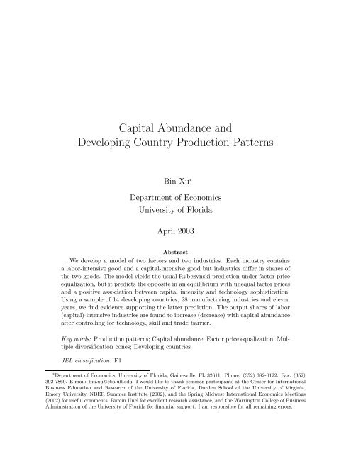
1992. Figure 1 depicts the average annual growth rates of industry value-added share in Chile
and Indonesia, with industries ranked in ascending order of capital intensity. The figure reveals
that on average labor-intensive industries expanded and capital-intensive industries contracted.
Such a pattern is found for seven of the 14 developing countries in our sample.
2

Moving beyond the simple correlation shown in Figure 1, we use regressions to isolate the
effect of capital abundance by controlling for other factors that influence production patterns.
Our empirical investigation uses the estimation approach of Harrigan and Zakrajšek (2000),
which is developed from the GDP function method of Diewert (1974) and Kohli (1978). The
Harrigan-Zakrajšek approach uses panel-data regressions to account for differences in technologies
and commodity prices without measuring them. In their study of the Rybczynski effects
in a sample of 21 industrialized countries and 7 relatively advanced developing countries (Argentina,
Chile, Hong Kong, Korea, Mexico, Turkey, and Taiwan) with four factors (unskilled
labor, skilled labor, capital, and land) and 10 sectors (grouped from 3-digit ISIC industries),
they found that the estimated Rybczynski effects have the expected signs in a significant number
of industries, particularly in large industries that are not natural-resource based.
Our finding contrasts sharply with that of Harrigan and Zakrajšek (2000). We find capital
abundance to be statistically significant in determining production patterns in 18 of the 28
industries (Table 3). However, the signs are opposite to what the standard HO model predicts.
In our full-sample panel-data regressions controlling for time and country fixed effects as well
as industry skill level (proxied by industry average wage rate relative to the US), the valueadded
shares of all of the 12 relatively labor-intensive industries increase with country capital
abundance, with six of them statistically significant, and the value-added shares of 12 of the 16
relatively capital-intensive industries decrease with country capital abundance, with six of the
12 statistically significant (Table 4).
A valid application of the Harrigan-Zakrajšek regression equation requires conditional factor
price equalization for countries in the sample. 1
Performing a test of conditional FPE that
estimates the correlation between industry capital intensity and country capital abundance in
1 If factor prices are not equalized conditional on technology differences, countries would produce different
sets of goods, and the estimated Rybczynski effect would switch signs with respect to different levels of capital
abundance (Leamer, 1987). Estimating a single Rybczynski equation in this case is not valid.
3

a pooled regression with industry fixed effects, 2 we reject the hypothesis of conditional FPE
for our full sample of 14 countries (Table 5). To search for a group of countries located in the
same cone that allows a legitimate application of the Harrigan-Zakrajšek regression equation, we
perform the conditional FPE test on different groups of countries in our sample, starting with a
pair of most labor-abundant countries (India and Indonesia). Adding labor-abundant countries
one by one, we find evidence of conditional FPE for the seven most labor-abundant countries
(Table 5). With conditional FPE holding for this subsample, we estimate a single Rybczynski
equation. The results show the same pattern as that of the full sample (Table 6). We find that
the value-added shares of 11 of the 13 relatively labor-intensive industries increase with country
capital abundance, with six of them statistically significant, and the value-added shares of 10 of
the 15 relatively capital-intensive industries decrease with country capital abundance, with five
of the 10 statistically significant. These results are contrary to the prediction of the standard
HO model but are consistent with the prediction of our non-FPE model. It is worth noting that
the kind of small open economy HO models with non-FPE were well discussed and analyzed in
Findlay (1973, chapter 9), Jones (1974), and Deardorff (1979) and more recently, in Findlay and
Jones (2001), and Deardorff (2001). The contribution of this paper is to develop such a model
that links observed industries to unobserved HO goods, use the model to predict a distinctively
difference response of industry production patterns to capital abundance, and provide empirical
evidence supporting the prediction of the model.
The remainder of the paper is organized as follows. In section 2 we develop a model that
allows a comparison of the output-endowment relationships under FPE and non-FPE. In section
3 we discuss the empirical approach and lay out the regression equation. In section 4 we describe
the data. In section 5 we present the results. In section 6 we conclude.
2 This test has been performed by Dollar, Wolff, and Baumol (1988) and Davis and Weinstein (2001). See
Harrigan (2001, p. 20) for a discussion of this test.
4

2 Theory
In this section we compare two models in their predictions on the output-endowment relationship
in a small open economy. One is the standard HO model with factor price equalization (FPE),
the other is an HO model with no factor price equalization (non-FPE).
Consider first the standard HO model of two factors, capital (K) and labor (L), and two
goods, capital-intensive X and labor-intensive Y . Suppose there are two industries, T (textiles)
and E (electronics). Our data identifies industries but not X and Y . Each industry contains
both labor-intensive and capital-intensive goods.
Assume that industry T has a share α of
good Y 1 , which is labor-intensive, and a share (1 − α) ofgoodX 1 , which is capital-intensive.
Similarly, E has a share β of labor-intensive good Y 2 and a share (1 − β) of capital-intensive
good X 2 . For our illustration, assume that Y 1 and Y 2 have the same capital intensity, so do X 1
and X 2 . Thus there are two “HO goods”, X = X 1 + X 2 and Y = Y 1 + Y 2 . Both α and β are
endogenously determined and we assume “no factor intensity reversal” of industries (α >β)in
the relevant equilibria. With these assumptions, we remain in the 2x2 HO framework. What is
new is that we distinguish HO goods (X and Y ) from industries (T and E). The Rybczynski
theorem states the relationship between (X, Y ) and capital abundance k ≡ K/L. Proposition
1 below establishes the relationship between (E, T ) and capital abundance k.
Proposition 1. In a FPE world, if capital abundance of a small open economy increases, the
capital-intensive industry E expands and the labor-intensive industry T contracts.
Consider next a non-FPE world. With unequal factor prices, trade leads to specialization.
A labor-abundant small open economy produces only the labor-intensive good Y . In our model
good Y can be Y 1 (labor-intensive textiles) or Y 2 (labor-intensive electronics). Without further
characterization of the two industries, the output of Y 1 and Y 2 cannot be determined. To break
up this indeterminacy, we introduce exogenous technology differences. Assume that good Y 1
5

and good Y 2 are identically priced at p 1 = p 2 = 1 in the world market because they have
identical unit labor and capital requirements based on world production technology. Assume,
however, that there is a gap between the labor-abundant country’s technology and the world’s
technology, and the gap is larger the higher the capital intensity of an industry. 3 Write the unit
cost function of good Y 1 as c 1 = c(w, r) and that of good Y 2 as c 2 = θd(w, r), where w and
r are the equilibrium wage and rental rates in the country, and θ>1 captures the relatively
large technology gap (measured by total factor productivity) of the country in sector E. For the
country to produce both Y 1 and Y 2 , the zero-profit conditions require c(w, r) =θd(w, r) =1.
It can be verified that the capital intensity of good Y 2 must be lower than that of good Y 1 to
offset its technology disadvantage associated the larger technology gap. Since good Y 1 is more
capital-intensive than good Y 2 , we can apply the Rybczynski theorem to establish:
Proposition 2. In a non-FPE world, a small open labor-abundant country specializes in laborintensive
goods. If there is a technology gap between the country and the world that is larger
the higher the capital intensity of an industry, and if the country produces in all industries, then
as the country becomes more capital-abundant, the labor-intensive industry T expands and the
capital-intensive industry E contracts.
Propositions 1 and 2 show the sharply different predictions of the two models on output
responses to endowment changes. One wonders to what extent these results can be generalized.
To get an idea, consider the case of two factors (capital and labor), n (> 2) goods, and j (> 2)
industries.
In the FPE model, with more goods than factors, there does not exist a unique
relationship between output and capital abundance. In the non-FPE model without technology
differences, a small open labor-abundant country will specialize in one labor-intensive good.
In the presence of the technology gap described in Proposition 2, the country will specialize
3 We assume this pattern of technology gap based on the belief that more capital-intensive industries tend to
be more technologically sophisticated.
6

in a set of labor-intensive goods that belong to different industries, with capital intensity of
the good in the country inversely related to the capital intensity of the industry in the world.
As in the FPE model, with more goods (industries) than factors, there does not exist a unique
relationship between output and capital abundance. This example indicates that a generalization
of Propositions 1 and 2 to higher dimensions is difficult. 4 Nevertheless, as now widely recognized,
the determinacy of output patterns is not a question of counting the numbers of goods and
factors, but a question that requires empirical estimation to settle (Harrigan, 2001, p. 15). 5
With this understanding, we set the issue aside and turn to empirical estimation to see if the
data reveals any systematic pattern.
3 Empirical Approach
In this section we describe a panel-data approach for estimating the effects of capital abundance
on output. This approach was developed by Harrigan and Zakrajšek (2000).
Consider a world of many countries, n factors, and n final goods. Factors are completely
mobile within a country but are completely immobile between countries. Consider a small open
economy that produces all n goods. World commodity prices are given by an nx1 vector P ∗ ,
and domestic prices are given by an nx1 vector P; these two price vectors may differ due to
trade barriers. Let W be an nx1 vector of domestic factor prices, and C(W) beannx1 vector
of unit cost functions. Production technologies are assumed to be neoclassical so the unit cost
functions are increasing, concave, and homogeneous of degree one in factor prices.
The unit cost functions imply an nxn production technique matrix A. The element of A is
a ij for good i and factor j, which is obtained from partial differentiation of good i’s unit cost
4 There can be a weak generalization however in the “even” case of equal number of factors and goods. Ethier
(1984) states this generalization as “endowment changes tend on average to increase the most those goods making
relatively intensive use of those factors which have increased the most in supply” (p. 168).
5 Bernstein and Weinstein (2002) is a pioneering paper to address empirically the question of output indeterminancy
in the HO model.
7

function with respect to factor j’s price. Let V be an nx1 vector of factor supplies, and Y be
an nx1 vector of good supplies. Perfect competition in factor markets leads to the following
full-employment conditions:
V = AY. (1)
With perfect competition in good markets, we also have the following zero-profit conditions:
P = C(W). (2)
Equations (1) and (2) characterize the general-equilibrium determination of W and Y at
given P and V. Assume that Nikaido’s (1972) condition is satisfied, we obtain from (2) a unique
solution of factor prices, W = C −1 (P). Provided that A is nonsingular at the equilibrium factor
prices, we obtain from (1) a unique solution of commodity supplies, Y = A −1 (W)V.
We are interested in the effects of factor supplies (V) on commodity supplies (Y), known as
“Rybczynski effects”. In this nxn model, using subscript 0 to denote the initial equilibrium and
1 the equilibrium after changes in factor supply, we have (Ethier, 1984, p. 167):
(V 1 − V 0 )A(W)(Y 1 − Y 0 ) > 0. (3)
This result says that factor supply changes will raise, on average, the output of goods relatively
intensive in those factors whose supply has increased the most and will reduce, on average, the
output of goods which make relatively little use of those factors whose supply has increased the
most. Notice that W has to remain the same in the two equilibria for this result to hold.
To estimate the Rybczynski effects, we use the GDP function method developed by Diewert
(1974) and Kohli (1978). With perfect competition, market-determined commodity outputs
equal the ones chosen by a social planner who maximizes gross domestic product. Let the GDP
function be G = G(p 1 ,p 2 , ...p n ,V 1 ,V 2 , ...V m ). If the GDP function is first-order differentiable,
its partial derivatives on commodity prices show the Rybczynski effects, and its partial derivatives
on factor supplies show the Stolper-Samuelson effects. Applying a second-order Taylor
8

approximation in logarithms to the GDP function yields a translog GDP function:
n∑
m∑
lnG = α 0 + α i lnp i + β k lnV k + 1 n∑ n∑
γ ij lnp i lnp j + 1 m∑ m∑
n∑ m∑
δ kl lnV k lnV l + φ ik lnp i lnV k .
2
2
i=1 k=1
i=1 j=1
k=1 l=1
i=1 k=1
(4)
Differentiating (4) with respect to lnp i yields an output share equation:
n∑
m∑
s i = α i + γ ij lnp j + φ ik lnV k , (5)
j=1
k=1
where s i ≡ dlnG/dlnp i = p i Y i /G i is the value-added share of good i in GDP. Note that homogeneity
properties imply ∑ n
i=1 α i =1, ∑ n
j=1 γ ij = 0, and ∑ m
k=1 φ ik =0.
3.1 Modeling Technology and Price Differences
So far we have been describing a single country with time-invariant technologies and commodity
prices. To isolate the effects of factor endowments on production patterns, we need to consider
differences in technologies and good prices across country and over time. We start by following
Harrigan (1987) in using an nx1 vector Θ to capture sector-specific Hicks-neutral technology
differences across countries (assumed constant over time).
In this case the GDP function is
written as G = G(θ 1 p 1 ,θ 2 p 2 , ...θ n p n ,V 1 ,V 2 , ...V m ), where θ i is an element of Θ. Using c as a
country subscript and t a time subscript we write the output share equation as
n∑
m∑
s ict = α i + b ic + γ ij lnp jct + φ ik lnV kct , (6)
j=1
k=1
where b ic ≡ ∑ n
j=1 γ ij lnθ jct is a country-specific constant that captures industry-specific Hicksneutral
technology differences across countries.
There are still non-neutral technology differences across countries and technology differences
across time. There are also differences in domestic good prices across countries and over time
due to trade barriers. To capture these differences, we follow Harrigan and Zakrajšek (2000) to
use an approximation for the price summation term in equation (6):
9

n∑
γ ij lnp jct = d ic + d it + η ict . (7)
j=1
Equation (7) assumes that at any time t, commodity price p ict differs across countries by a
country-specific parameter d ic ; this can be a result of a non-neutral technology difference or
a trade-barrier difference. It also allows commodity price p ict to differ across time by a timespecific
(but common across countries) parameter d it ; this captures the time variation of global
technologies and trade barriers. There remain country-specific time-variant price differences; we
model them by an error term η ict . Substituting (7) into (6) yields
m∑
s ict = α i + δ ic + d it + φ ik lnV kct + η ict , (8)
k=1
where δ ic = b ic + d ic captures the combined effect of cross-country time-invariant (neutral and
non-neutral) technology differences and price differences.
3.2 Estimation Equation
For our purpose, we need to derive an estimation equation with two factors from the n-factor
model. To do so, we assume that the n factors belong to two categories, labor and capital.
Let K be the aggregation of various capital factors, and L be the aggregation of various labor
factors. Both capital and labor are heterogeneous. We consider sophistication of capital as
part of “technologies” and assume heterogeneity of labor in industry-specific skill. Industry i in
country c employs L hic skilled workers who are immobile between industries and L lic unskilled
workers who are mobile between industries. We will make output share of industry i dependent
on industry skill level h ic and treat L c = ∑ i (L hic +L lic ) as country c’s labor endowment. Taking
these considerations into account, we obtain the following output share equation:
s ict = α i + δ ic + d it + φ i ln(K/L) ct + ρ i lnh ict + ε ict . (9)
10

Equation (9) is the regression equation for our estimation. With data pooled over countries and
time, the output share of industry i depends on country-specific effects δ ic , time-specific effects
d it , capital abundance (K/L) ct , industry skill level h ict , and all other remaining factors ε ict .
4 Data
The data for our study are mainly from UNIDO Industrial Statistics Database (3-Digit ISIC
Code, 1963-1999) and the World Bank Trade and Production Database (3-Digit ISIC Code, 1976-
1999). 6 The production data in the World Bank database are the same as those in the UNIDO
database, but the World Bank database also contains trade data in 3-Digit ISIC Code. The data
in these two databases are in current U.S. dollars. Penn World Tables provide price parities for
value added and investment.
We use them to convert all current values to internationally
comparable values in 1985 international dollar.
All capital stocks are computed using the perpetual inventory method, with 1975 as the
initial year and 10% as the discount rate. Industry capital stocks are computed from UNIDO
industry-level investment data. Country capital stocks are computed from investment data in
the Penn World Tables. Our sample contains 14 developing countries (Table 1). These are
the only 14 developing countries that have a relatively complete industry-level investment series
from which we construct industry capital stocks. The sample period is 1982-1992. 7
For each industry we calculate its value-added share in total manufacturing. We also calculate
the wage rate relative to the U.S. as a proxy for the skill level of an industry, and exports plus
imports in manufacturing value added as a measure of industry trade openness. At the 3-digit
ISIC level every country exports and imports in every industry.
6 See Nicita and Olarreaga (2001) for the document of the World Bank database.
7 We choose 1982 as the beginning year because the investment series starts in 1975 for most of the countries
and we need several years of investment accumulation for estimated capital stocks to be relatively insensitive to
initial-year investment. The choice of 1992 is because it is the ending year of the Penn World Tables.
11

5 Empirical Results
5.1 Estimating Rybczynski Effects: Full Sample
In Table 3 we report results from estimating equation (9) using both fixed-effects and randomeffects
methods. The results are quite similar between the two methods. The Hausman test
supports the hypothesis of no correlation between the independent variables and the countryspecific
effects in almost all cases, so the random-effects estimator is valid. As Harrigan and
Zakrajšek (2000) point out, the random-effects estimator is useful because it captures some of
the cross-country variation in the data.
Table 3 shows our main finding: capital abundance (K/L) tends to have a positive effect
on the value-added shares of relatively labor-intensive manufactured industries, and a negative
effect on the value-added shares of relatively capital-intensive manufactured industries. In 14
of the 16 most labor-intensive industries, the estimated effects of (K/L) are positive, and 11 of
them are statistically significant (random-effects estimation). In nine of the 12 most capitalintensive
industries, the estimated effects of (K/L) are negative, and four of them are negative
and statistically significant. This finding is contrary to the prediction of the standard HO model
but consistent with the prediction of our non-FPE model (Proposition 2).
In Table 3 we do not control for the skill level of the labor force. If an industry is laborintensive
due to intensive use of skilled labor, then an increase in a country’s capital abundance,
often accompanied by an increase in its skill abundance, can lead to a positive correlation
between output shares and (K/L). Harrigan and Zakrajšek (2000) distinguish skilled labor and
unskilled labor.
As we argue in section 2, if skilled labor is industry-specific, then we may
control for its effect using an industry skill measure. The industry average wage rate relative to
the U.S. provides a proxy for industry skill level. Table 4 reports results from regressions that
include this skill variable. We find the same pattern as that of Table 3. Only two industries
see noticeable changes: the estimated effect of (K/L) on textiles (321) turns from positive and
12

statistically significant without controlling for skill to negative and statistically insignificant
with skill controlled for, and the estimated effect of (K/L) on fabricated metal products (381)
turns from positive and statistically significant to positive and statistically insignificant. The
estimated effects of the skill variable are statistically significant in 14 of the 28 industries, with
nine of the 14 showing a positive estimated coefficient, suggesting that most manufacturing
industries would see output share to increase with skill.
5.2 Identifying a Subsample with Conditional FPE
Estimating a single Rybczynski equation (9) is valid only if factor prices are conditionally equalized
in the sample. Otherwise countries would produce different sets of goods and the estimated
Rybczynski effect would switch signs with respect to different levels of capital abundance.
The literature offers a simple test of conditional FPE. Under conditional FPE, countries
produce the same set of goods. A change in factor supplies will be fully absorbed by outputshare
adjustments, leaving factor prices unchanged.
As a result, production techniques will
be insensitive to factor-supply changes.
This suggests, in the two-factor case, the following
regression equation for testing the conditional FPE hypothesis:
( )
( )
K K
= α it + β t + ν ict . (10)
L ict L ct
In regression equation (10), the dependent variable is industry capital intensity, and the independent
variable is country capital abundance. Pooling data across country and industry for
any time t, we have industry capital intensity (K/L) ict dependent on industry-specific fixed
effects α it . 8 Under the null hypothesis of conditional FPE, we have β t = 0. The error term ν ict
is assumed to be zero-mean random technology shocks. If there is no conditional FPE, then
β t ̸= 0. In particular, non-FPE models (e.g. Dornbusch, Fischer, and Samuelson, 1980) predict
8 The regression does not include country-specific fixed effects because neutral technology differences across
countries do not affect capital intensity.
13

that β t > 0: the goods produced by a labor-abundant country are more labor-intensive than the
goods produced by a capital-abundant country.
Table 5 reports results from estimating (10). The first row of Table 5 reports the results
for the full sample of 14 countries. We find that the estimated β is positive and statistically
significant at the 1 percent level, clearly rejecting conditional FPE in the full sample. 9
One reason for factor prices not equalized is that countries have very different capital abundance.
To see if conditional FPE holds for a subsample of countries which have similar capital
abundance, we apply regression (10) first to a pair of most labor-abundant countries, India and
Indonesia. The estimated β is positive, but the statistical significance level is only 10 percent.
If we add to the sample the next labor-abundant country, Egypt, then the estimated β becomes
statistically indifferent from zero. Continuing this experiment, we find that the estimated β is
indifferent from zero for the subsample of the seven most labor-abundant countries in 1992. This
is true in 1982 as well. These results suggest that conditional FPE holds among the seven most
labor-abundant countries in our sample. Their capital abundance is similar enough for them to
produce similar goods. Table 5 also shows some evidence that the three most capital-abundant
countries (Korea, Hong Kong, and Singapore) form a single cone of diversification.
5.3 Estimating Rybczynski Effects: Subsample
Given conditional FPE in the subsample of the seven most labor-abundant countries, we can
run a single Rybczynski regression on this subsample. Table 6 reports the results. 10 We find the
9 We also use the decomposition method of Hanson and Slaughter (2002). The method is to decompose the
changes in factor supply into output-mix changes, generalized changes in production techniques, and idiosyncratic
changes in production techniques. In their examination of U.S. states, Hanson and Slaughter find that statespecific
changes in production techniques play a relatively small role and interpret it as evidence of conditional
FPE among U.S. states. Our results show that country-specific changes in production techniques play a relatively
large role (40% for labor and 29% for capital, averaged over the 14 countries for the period 1982-1992), which
supports our rejection of conditional FPE for countries in our sample.
10 The industries in Table 6 are ranked in ascending order of average capital intensity of the subsample. The
second and third columns compare the industry capital intensities between the full sample and the subsample.
The average capital intensity of the 7 most labor-abundant country is significantly lower than that of the full
sample, but the ranking is largely the same.
14

same pattern as in the full sample: labor-intensive manufacturing industries tend to expand and
capital-intensive manufacturing industries tend to shrink as capital abundance increases. The
value-added shares of 11 of the 13 relatively labor-intensive industries increase with country
capital abundance, with six of them statistically significant, and the value-added shares of 10 of
the 15 relatively capital-intensive industries decrease with country capital abundance, with five
of the 10 statistically significant.
In our output share regressions we use time dummies to control for unobserved time-specific
factors common to all countries, and country dummies to control for unobserved country-specific
factors common across time. There remain country-specific time-variant unobserved factors that
may affect the identification of the role of capital abundance. One such factor is trade barrier.
For developing countries a lower trade barrier generally means more exports of labor-intensive
goods and less imports of capital-intensive goods. If trade openness is positively correlated with
capital abundance, then as a country becomes more abundant in capital it exports more laborintensive
goods and imports less capital-intensive goods, thus producing more labor-intensive
goods and less capital-intensive goods. In fact, trade openness is found to have increased more in
labor-intensive industries than in capital-intensive industries in seven of the 14 sample countries.
Figure 2 depicts changes in industry trade openness in Chile and Indonesia, with the horizontal
axis showing industries ranked in ascending order of capital intensity.
To control for the effect of industry-specific trade barrier that differs across country and over
time, we introduce an additional independent variable T ict defined as industry trade openness.
In Table 7 we use industry exports plus imports in manufacturing value-added as a measure of
industry trade openness. We find this variable to have a positive and statistically significant
effect on value-added share of 11 industries, and a negative and statistically significant effect on
one industry (371, iron and steel). We find, however, that adding this trade openness variable,
while reducing the point estimates of the effects of capital abundance, does not change the
15

signs of the effects. Capital abundance still has a positive and statistically significant effect on
five labor-intensive industries, and a negative and statistically significant effect on six capitalintensive
industries. The pattern remains to be the one contrary to the prediction of the standard
HO model but consistent with the prediction of our non-FPE model. 11
6 Conclusion
Recent empirical studies confirm the significance of factor abundance in understanding global
production and trade but find technology and “multiple cones” equally significant, if not more.
While the theoretical literature has long recognized it, it lacks a simple model that melts all
these three elements and serves as a compelling alternative to the standard HO model. Such a
model is especially needed for analyzing open developing economies, which face technology gaps
and produce a mix of goods different from those produced by developed countries.
This paper is a small step toward this gigantic goal. We develop a model that distinguishes
goods from industries. Goods are homogeneous but industries are not. With certain assumptions
the model can be made equivalent to the 2x2 HO model, and has the implication that
under FPE, an increase in the supply of a factor increases the output of the industry that uses
intensively the factor and decreases the output of the other industry (at constant goods prices).
By distinguishing between goods and industries, the model implies that a small open economy,
under non-FPE, will produce only the goods with factor intensity equal to its factor abundance,
and yet have positive production in all industries. This fills a gap between the prediction of
the small open economy HO model that a country, under non-FPE, produces only one good
11 We check the robustness of our results using data on aggregate capital stocks from Penn World Tables 5.6,
which are available for nine of the 14 countries. Following Harrigan and Zakrajšek (2000) we aggregate producer
durables and non-residential construction. The correlation between this capital stock measure and the measure
constructed from investment series is 0.61. When this capital stock measure is used, only four estimated coefficients
on log(K/L) are statistically significant. The pattern remains in that the estimated coefficients are positive for
the two relatively labor-intensive industries (381 and 383) and negative for the two relatively capital-intensive
industries (352 and 362).
16

(no more than two to be precise), and the observation that no country produces in a single
industry (no matter how disaggregate the data is).
Moreover, introducing a technology gap
between the developing country and the world and assuming a positive correlation between the
size of the gap and the capital intensity of the industry, the model yields a surprising prediction
on the response of industry output to factor abundance. The model predicts, under non-FPE
and the assumed pattern of technology gap, that an increase in the capital abundance of a
small open labor-abundant country will expand its labor-intensive industry and contract its
capital-intensive industry, contrary to the prediction of the standard HO model.
This surprising prediction finds empirical support from our investigation of a sample of 14
developing countries and 28 manufacturing industries over the period 1982-1992. Using a paneldata
approach to control for unobserved country-specific and time-specific changes in technology,
resources other than capital and labor, trade barriers, and others, as well as the observed changes
in industry skill level and trade openness (that are neither country-specific nor time-specific),
we find a pattern that is consistent with the prediction of our non-FPE model. The shares of
labor-intensive industries tend to increase and the shares of capital-intensive industries tend to
decrease, as country capital abundance increases.
Admittedly there are both theoretical and empirical unresolved issues regarding the validity
of our finding. For example, our theoretical predictions derived from a two-dimension model
seem difficult to generalize to higher dimensions. Large measurement errors exist in our data,
particularly in capital stocks.
The panel-data approach and our measure of industry trade
openness may not capture the entire effect from trade barriers. And there are factors such as
foreign direct investment that may be important but are not controlled for. All said, the unusual
regularity found in the data is remarkable to this author and the results are worth reporting
and can serve as a motivation for future theoretical modeling and empirical investigation.
17

References
Bernstein, Jeffrey R. and David E. Weinstein (2002), “Do Endowments Predict the Location
of Production? Evidence from National and International Data,” Journal of International Economics,
56(1), 57-76.
Davis, Donald R. and David E. Weinstein (2001), “An Account of Global Factor Trade,” American
Economic Review, 91(5), 1423-1453.
Deardorff, Alan V. (1979), “Weak Links in the Chain of Comparative Advantage,” Journal of
International Economics, 9, 197-209.
Deardorff, Alan V. (2001), “Developing Country Growth and Developed Country Response,”
Journal of International Trade and Economic Development, 10(4), 373-392.
Diewert, W. Erwin (1974), “Applications of Duality Theory,” in M. Intriligator and D. Kendrick,
eds., Frontiers of Quantitative Economics, North-Holland, Amsterdam, 106-171.
Dollar, David, Edward N. Wolff, and William J. Baumol (1988), “The Factor-Price Equalization
Model and Industry Labor Productivity: An Empirical Test across Countries,” in Robert C.
Feenstra, ed., Empirical Methods for International Trade, MIT Press, Cambridge, MA, 23-47.
Dornbusch, Rudiger, Stanley Fischer, and Paul A. Samuelson (1980), “Heckscher-Ohlin Trade
Theory with a Continuum of Goods,” Quarterly Journal of Economics, 95, 203-224.
Ethier, Wilfred J. (1984), “Higher Dimensional Issues in Trade Theory,” in Ronald W. Jones
and Peter B. Kenen, eds., Handbook of International Economics, North-Holland, Amsterdam,
131-184.
Findlay, Ronald (1973), International Trade and Development Theory, Columbia University
Press, New York.
Findlay, Ronald and Ronald W. Jones (2001), “Economic Development from an Open Economy
Perspective,” in Deepak Lal and Richard Snape, eds., Trade, Development and Political
Economy, Palgrave Press.
Hanson, Gordon H. and Matthew J. Slaughter (2002), “Labor-Market Adjustment in Open
Economies: Evidence from U.S. States,” Journal of International Economics, 57(1), 3-29.
18

Harrigan, James (1997), “Technology, Factor Supplies and International Specialization: Estimating
the Neoclassical Model,” American Economic Review, 87(4), 475-494.
Harrigan, James (2001), “Specialization and the Volume of Trade: Do the Data Obey the Laws?”
NBER Working Paper No. 8675.
Harrigan, James and Egon Zakrajšek (2000), “Factor Supplies and Specialization in the World
Economy,” NBER Working Paper No. 7848.
Jones, Ronald W. (1974), “The Small Country in a Multi-Commodity World,” Australian Economic
Papers, 13, 225-236.
Jones, Ronald W. (1999), “Heckscher-Ohlin Trade Models for the New Century”, mimeo, University
of Rochester.
Kohli, Ulrich R. (1978), “A Gross National Product Function and the Derived Demand for
Imports and Supply of Exports,” Canadian Journal of Economics, 11, 167-182.
Leamer, Edward E. (1987), “Paths of Development in the Three-Factor, n-Good General Equilibrium
Model,” Journal of Political Economy, 95, 961-999.
Nicita, Alessandro and Marcelo Olarreaga (2001), “Trade and Production, 1976-1999,” mimeo,
World Bank.
Nikaido, Hukukane (1972), “Relative Shares and Factor Price Equalization,” Journal of International
Economics, 2(3), 257-263.
Rybczynski, T. M. (1955), “Factor Endowments and Relative Commodity Prices,” Economica,
22, 336-341.
Schott, Peter K. (2001), “One Size Fits All? Heckscher-Ohlin Specialization in Global Production,”
NBER Working Paper No. 8244.
19

.2
354
.1
gsy
0
361
390
356
384
332
385
382
322
321
381
331 311 362 383
324
352313
355
342
351
369
353
341
372
323
314
371
-.1
0 20 40 60
akl
Chile
.2
332
324
385
.1
322
390
356
341
gsy
323
361
0
311
331
355
383 321 342
381
382
384
351
314
362
352
313
369
-.1
0 5 10 15
akl
Indonesia
Figure 1. Average Annual Growth in Industry Value-Added Share (gsy)
with Industries Ranked in Order of Average Capital Intensity (akl), 1982-1992

.2
331
323
.1
gty
0
332
321361
356 362
355 313
384
324 390 342 383
382
381 352
322
354
385
311
351
369
341
371
314
372
-.1
353
0 20 40 60
akl
Chile
.4
324
.2
332
323
322
gty
314
356
321 342
361
390
331
0
355
385
352
383
382 381
311
313
384
362
341
351
369
371
-.2
0 5 10 15
akl
Indonesia
Figure 2. Average Annual Growth in Industry Trade Openness (gty)
with Industries Ranked in Order of Average Capital Intensity (akl), 1982-1992

Table 1. Countries in the Sample
Capital Abundance Rank Country
Capital Abundance (K/L)
(Low to High)
1982-1992 average 1982 1992
1 India 0.204 0.147 0.295
2 Indonesia 0.410 0.180 0.770
3 Egypt 0.429 0.342 0.404
4 Philippines 0.638 0.538 0.701
5 Colombia 0.792 0.643 0.817
6 Chile 0.812 0.604 1.233
7 Turkey 0.840 0.652 0.937
8 Malaysia 1.347 0.790 2.269
9 Hungary 1.714 1.303 2.123
10 Ecuador 1.801 1.821 1.899
11 Poland 1.879 2.096 2.093
12 Korea 2.183 1.270 3.438
13 Hong Kong 2.387 1.452 3.526
14 Singapore 6.494 4.312 7.694
Table 2. Industries in the Sample
L i /K i ISIC Industry
Value-added
Capital Intensity
Rank code
share 82-92 average 1982 1992
1 322 Wearing apparel except footwear 0.039 2.454 1.810 3.493
2 324 Footwear except rubber or plastic 0.007 4.126 3.141 6.281
3 332 Furniture except metal 0.008 4.980 3.731 10.809
4 390 Other manufactured products 0.011 6.591 6.090 8.441
5 323 Leather products 0.004 6.969 6.878 9.611
6 385 Professional and scientific equipment 0.012 8.658 6.661 12.144
7 381 Fabricated metal products 0.042 9.173 6.758 11.869
8 382 Machinery except electric 0.052 9.297 7.932 12.320
9 331 Wood products except furniture 0.023 9.369 8.506 10.965
10 342 Printing and publishing 0.025 10.167 8.061 13.194
11 356 Plastic products 0.023 10.795 8.316 14.667
12 361 Pottery china earthenware 0.005 10.983 10.601 11.676
13 321 Textiles 0.087 11.317 8.683 15.098
14 311 Food products 0.119 11.934 9.669 14.528
15 383 Machinery electric 0.093 12.113 9.047 18.710
16 384 Transport equipment 0.054 13.051 9.505 16.842
17 355 Rubber products 0.019 13.327 9.138 20.865
18 352 Other chemicals 0.054 14.185 10.374 20.355
19 313 Beverages 0.046 18.223 13.258 27.792
20 362 Glass and products 0.009 18.708 13.889 27.433
21 314 Tobacco 0.036 19.033 12.887 25.475
22 341 Paper and products 0.025 21.256 15.500 33.222
23 369 Other non-metallic mineral products 0.037 26.010 19.690 31.864
24 372 Non-ferrous metals 0.028 29.967 21.319 41.192
25 354 Misc. petroleum/coal products 0.007 30.424 20.203 55.979
26 371 Iron and steel 0.043 37.481 32.740 46.689
27 351 Industrial chemicals 0.046 38.869 30.175 55.833
28 353 Petroleum refineries 0.068 98.680 58.511 171.147

Table 3. Panel Regressions, Industry Value-Added Share, 14 Countries, 1982-1992
L i /K i ISIC
Random-Effects
Estimation
Fixed-Effects
Estimation
ln(K/L) R 2 R 2 ln(K/L) R 2
rank code Effect of Between Within Effect of Within
(Prob. rejecting H 0 )
1 322 −0.003 0.108 0.027 −0.005 0.029 154 0.002
(0.005)
(0.005)
2 324 0.003 0.000 0.167 0.006 0.186 154 0.408
(0.001)***
(0.002)***
3 332 0.006 0.379 0.244 0.008 0.248 154 0.099
(0.001)***
(0.001)***
4 390 0.005 0.301 0.165 0.005 0.166 154 0.000
(0.002)***
(0.002)**
5 323 0.0014 0.018 0.132 0.002 0.136 154 0.003
(0.0005)***
(0.0007)***
6 385 0.004 0.230 0.102 0.002 0.103 154 0.000
(0.002)**
(0.002)
7 381 0.009 0.507 0.117 0.007 0.119 154 0.000
(0.002)***
(0.003)*
8 382 0.023 0.236 0.107 0.022 0.107 154 0.000
(0.009)***
(0.014)
9 331 0.005 0.073 0.102 0.008 0.106 154 0.008
(0.004)
(0.004)*
10 342 0.005 0.340 0.051 0.002 0.055 154 0.001
(0.002)**
(0.003)
11 356 0.006 0.206 0.081 0.005 0.081 154 0.000
(0.002)**
(0.0024)
12 361 0.001 0.002 0.105 0.002 0.105 142 0.000
(0.001)
(0.001)
13 321 0.004 0.228 0.342 0.015 0.351 154 0.244
(0.007)
(0.008)*
14 311 −0.022 0.179 0.027 −0.016 0.028 152 0.000
(0.012)*
(0.017)
15 383 0.043 0.450 0.097 0.032 0.099 154 0.000
(0.012)***
(0.015)**
16 384 0.011 0.022 0.085 0.014 0.086 154 0.000
(0.005)**
(0.006)**
17 355 −0.003 0.064 0.170 −0.0024 0.170 154 0.000
(0.002)
(0.003)
18 352 −0.013 0.218 0.108 −0.014 0.108 154 0.000
(0.004)***
(0.005)**
19 313 0.137 0.001 0.177 0.016 0.177 154 0.000
(0.006)**
(0.007)**
20 362 −0.0003 0.000 0.113 −0.0006 0.114 143 0.000
(0.0009)
(0.0011)
21 314 −0.019 0.231 0.158 −0.020 0.158 154 0.000
(0.006)***
(0.008)**
22 341 0.009 0.024 0.285 0.012 0.293 154 0.490
(0.002)***
(0.002)***
23 369 −0.004 0.115 0.117 −0.002 0.118 154 0.000
(0.003)
(0.004)
24 372 −0.001
(0.008)
0.054 0.135 0.002
(0.009)
0.136 146 0.000

25 354 0.0004
(0.0019)
26 371 −0.019
(0.005)***
27 351 −0.005
(0.005)
28 353 −0.036
(0.019)**
0.070 0.169 0.006
(0.0034)**
0.418 0.189 −0.022
(0.008)***
0.152 0.134 .0010
(0.007)
0.004 0.339 −0.169
(0.040)***
0.197 116 0.051
0.189 143 0.000
0.138 154 0.000
0.304 121 0.773
Notes: The dependent variable is industry value-added share. The fixed-effects estimation uses country-specific
and time-specific dummies as independent variables. The random-effects estimation uses time-specific dummies
as independent variables and a random country-specific error component. Asterisks indicate statistical significance
level, with *** for less than 1 percent, ** for less than 5 percent, and * for less than 10 percent. The Hausman
specification test is performed to test the null hypothesis H 0 that there is no systematic difference between
estimated coefficients from the fixed-effects estimator and those from the random-effects estimator, provided that
the model is correctly specified and there is no correlation between the independent variables and the countryspecific
effects.

Table 4. Panel Regressions, Industry Value-Added Share, 14 Countries, 1982-1992
L i /K i ISIC Random-Effects Estimation
rank code Effect of ln(K/L) Effect of ln(w c /w US)
1 322 0.000
−0.003
(0.006)
(0.003)
2 324 0.005
−0.002
(0.001)*** (0.001)***
3 332 0.005
0.0004
(0.001)***
(0.001)
4 390 0.007
−0.003
(0.002)*** (0.001)***
5 323 0.001
0.0004
(0.0006)**
(0.0003)
6 385 0.004
0.000
(0.002)**
(0.001)
7 381 0.006
0.005
(0.003)** (0.002)**
8 382 0.016
0.012
(0.010)
(0.007)*
9 331 0.005
−0.001
(0.004)
(0.002)
10 342 0.0002
0.010
(0.002)
(0.002)***
11 356 0.005
0.001
(0.003)
(0.002)
12 361 0.001
0.001
(0.001)
(0.001)
13 321 −0.001
0.008
(0.008)
(0.005)
14 311 −0.030
0.014
(0.013)**
(0.008)*
15 383 0.046
−0.009
(0.012)***
(0.008)
16 384 0.011
−0.000
(0.006)**
(0.004)
17 355 −0.003
0.001
(0.002)
(0.001)
18 352 −0.018
0.014
(0.004)*** (0.003)***
19 313 0.010
0.010
(0.006)* (0.003)***
20 362 −0.002
0.002
(0.001)* (0.001)***
21 314 −0.029
0.012
(0.007)*** (0.004)***
22 341 0.011
−0.005
(0.002)*** (0.001)***
23 369 −0.008
0.009
(0.003)*** (0.002)***
24 372 −0.009
0.008
(0.008)
(0.004)**
25 354 −0.002
0.002
(0.002)
(0.001)
Between R 2 Within R 2 n
0.323 0.037 154
0.007 0.226 154
0.349 0.255 154
0.256 0.228 154
0.018 0.139 154
0.230 0.102 154
0.525 0.147 154
0.165 0.132 154
0.057 0.103 154
0.508 0.226 154
0.239 0.082 154
0.005 0.121 142
0.000 0.350 154
0.200 0.049 152
0.446 0.105 154
0.022 0.086 154
0.042 0.174 154
0.234 0.246 154
0.006 0.238 154
0.010 0.244 143
0.140 0.231 154
0.104 0.386 154
0.042 0.241 153
0.295 0.153 146
0.498 0.145 116

26 371 −0.018
(0.006)***
27 351 −0.004
(0.005)
28 353 −0.030
(0.020)
−0.002
(0.004)
−0.002
(0.003)
−0.049
(0.014)***
0.432 0.189 143
0.143 0.136 154
0.001 0.347 121

Table 5. Pooled Regressions, OLS with Robust Standard Errors
Countries in regression
1992 1982
Country code: (K/L) rank Estimated β Adjusted R 2 Estimated β Adjusted R 2
All countries 5.035
(0.839)***
0.396 3.039
(0.522)***
0.437
1, 2 4.359
(2.520)*
1, 2, 3 4.319
(4.001)
1, 2, 3, 4 −0.675
(6.037)
1, 2, 3, 4, 5 −2.549
(5.242)
1, 2, 3, 4, 5, 6 2.042
(4.541)
1, 2, 3, 4, 5, 6, 7
2.392
(K/L < 1)
(4.256)
(1, 2, 3, 4, 5, 6, 7) + 8 8.261
(3.774)**
8, 9 113.787
(70.214)
8, 9, 10 57.904
(52.122)
8, 9, 10, 11
−96.053
(1 < K/L < 2)
(34.886)***
(8, 9, 10, 11) + 12 7.879
(4.877)*
12, 13 −257.848
(106.274)**
12, 14 −2.921
(1.536)*
12, 13, 14
−0.385
(K/L > 2)
(1.264)
(12, 13, 14) + 11 2.230
(0.960)**
Note: Country code is the one displayed in Table 1.
0.910 12.641
(33.572)
0.479 72.279
(13.038)***
0.510 6.689
(5.532)
0.521 1.344
(3.801)
0.470 3.024
(3.967)
0.497 2.235
(3.164)
0.497 0.258
(2.449)
0.168 18.373
(6.785)***
0.242 9.046
(2.138)***
0.392 11.132
(2.090)***
0.313 10.732
(1.5686)***
0.825 −36.106
(14.313)**
0.913 −0.339
(0.678)
0.827 0.562
(0.576)
0.371 0.422
(0.589)
0.594
0.549
0.231
0.377
0.283
0.316
0.333
0.508
0.649
0.470
0.509
0.803
0.865
0.783
0.713

Table 6. Random-Effects Panel Regressions, Industry Value-Added Share, 7 Countries, 1982-1992
L i /K i
rank
ISIC
code
Capital
Intensity
(14C)
Capital
Intensity
(7C)
Effect of
ln(K/L)
1 322 2.454 1.636 0.003
(0.005)
2 332 4.980 2.296 0.006
(0.001)***
3 324 4.126 2.599 0.009
(0.001)***
4 323 6.969 4.560 0.001
(0.001)**
5 390 6.591 4.902 0.002
(0.001)**
6 385 8.658 5.095 −0.001
(0.001)
7 381 9.173 5.383 −0.002
(0.005)
8 331 9.369 5.642 0.018
(0.007)***
9 382 9.297 6.052 0.001
(0.005)
10 356 10.795 6.402 0.003
(0.003)
11 311 11.934 6.519 0.023
(0.014)*
12 321 11.317 7.161 0.002
(0.012)
13 342 10.167 7.431 0.002
(0.003)
14 383 12.113 8.523 −0.009
(0.008)
15 352 14.184 8.574 −0.022
(0.007)***
16 355 13.327 8.984 −0.004
(0.003)
17 384 13.051 9.191 −0.001
(0.007)
18 362 18.708 9.354 −0.002
(0.001)*
19 313 18.223 9.608 0.015
(0.008)*
20 314 19.033 10.057 −0.028
(0.012)**
21 361 10.983 10.761 0.001
(0.001)
22 341 21.256 17.577 0.022
(0.004)***
23 354 30.424 20.533 0.002
(0.004)
24 369 26.010 21.060 −0.011
(0.005)**
Effect of
ln(w c /w US)
0.008
(0.003)**
0.001
(0.001)
−0.002
(0.001)***
0.001
(0.0004)***
−0.000
(0.001)
0.001
(0.0004)***
0.004
(0.003)
−0.001
(0.004)
0.005
(0.003)*
0.002
(0.002)
0.011
(0.008)
0.007
(0.007)
0.005
(0.002)***
0.008
(0.005)*
0.017
(0.004)***
0.001
(0.001)
0.008
(0.004)**
0.003
(0.001)***
0.015
(0.004)***
0.006
(0.006)
0.002
(0.001)***
−0.005
(0.002)**
0.003
(0.002)
0.010
(0.003)***
Between
R 2
Within
R 2
0.034 0.469 77
0.177 0.510 77
0.064 0.630 77
0.033 0.266 77
0.2013 0.268 77
0.095 0.261 77
0.1057 0.181 77
0.019 0.213 77
0.026 0.214 77
0.049 0.249 77
0.182 0.211 77
0.071 0.335 77
0.120 0.305 77
0.004 0.183 77
0.010 0.358 77
0.009 0.138 77
0.124 0.296 77
0.060 0.285 77
0.234 0.282 77
0.050 0.331 77
0.351 0.279 77
0.161 0.512 77
0.375 0.235 77
0.094 0.311 77
n

25 372 29.967 22.271 0.007
(0.020)
26 351 38.869 25.174 −0.007
(0.006)
27 371 37.481 31.692 −0.036
(0.013)***
28 353 98.680 66.305 −0.030
(0.043)
0.012
(0.008)
−0.009
(0.004)***
−0.007
(0.006)
−0.065
(0.020)***
0.387 0.266 69
0.361 0.203 77
0.435 0.354 69
0.120 0.369 77
Note: The third column shows the capital intensity of an industry averaged over the 14 countries, and the fourth
column shows the capital intensity of an industry averaged over the seven countries.

Table 7. Random-Effects Panel Regressions, Industry Value-Added Share, 7 Countries, 1982-1992
L i /K i
rank
ISIC code Effect of
ln(K/L)
1 322 0.003
(0.005)
2 332 0.003
(0.001)***
3 324 0.007
(0.001)***
4 323 0.001
(0.0007)*
5 390 0.002
(0.001)**
6 385 −0.001
(0.001)
7 381 −0.001
(0.004)
8 331 0.014
(0.007)**
9 382 0.0002
(0.005)
10 356 0.004
(0.004)
11 311 0.027
(0.015)*
12 321 −0.007
(0.012)
13 342 −0.0003
(0.002)
14 383 −0.003
(0.007)
15 352 −0.016
(0.007)**
16 355 −0.003
(0.003)
17 384 0.0003
(0.007)
18 362 −0.002
(0.001)
19 313 0.016
(0.008)**
20 314 −0.045
(0.013)***
21 361 0.001
(0.001)
22 341 0.021
(0.004)***
23 354 0.004
(0.004)
24 369 −0.012
(0.004)***
25 372 0.025
(0.018)
Effect of
ln(w c /w US)
0.011
(0.004)***
0.001
(0.0007)*
−0.002
(0.001)**
0.001
(0.0004)**
−0.0004
(0.001)
0.001
(0.0004)***
0.004
(0.003)
0.001
(0.004)
0.005
(0.003)*
0.002
(0.002)
0.011
(0.008)
0.018
(0.008)**
0.006
(0.001)***
0.009
(0.005)**
0.018
(0.004)***
0.001
(0.001)
0.009
(0.004)**
0.003
(0.001)***
0.015
(0.004)***
0.004
(0.006)
0.002
(0.001)***
−0.005
(0.002)**
0.001
(0.002)
0.009
(0.002)***
0.029
(0.009)
Effect of
ln(T/Y)
0.004
(0.002)*
0.001
(0.0004)***
0.001
(0.0004)***
0.0002
(0.0002)
0.0002
(0.0003)
−0.001
(0.0004)*
0.003
(0.002)
0.006
(0.002)***
0.002
(0.002)
−0.001
(0.002)
0.006
(0.008)
0.028
(0.008)***
0.004
(0.001)***
0.011
(0.003)***
0.012
(0.004)***
0.004
(0.002)**
0.0004
(0.003)
0.001
(0.001)
0.004
(0.002)*
0.008
(0.003)***
0.0008
(0.0003)**
−0.0004
(0.001)
−0.001
(0.001)
0.004
(0.001)***
0.015
(0.006)***
Between
R 2
Within
R 2
0.194 0.476 77
0.486 0.497 77
0.063 0.678 77
0.070 0.259 77
0.082 0.262 77
0.182 0.288 77
0.344 0.199 77
0.248 0.261 77
0.042 0.226 77
0.051 0.252 77
0.259 0.212 77
0.493 0.418 77
0.678 0.350 77
0.039 0.322 77
0.022 0.442 77
0.008 0.225 77
0.230 0.304 77
0.191 0.302 77
0.329 0.312 77
0.001 0.416 77
0.256 0.352 77
0.151 0.513 77
0.200 0.278 69
0.498 0.391 77
0.868 0.113 69
n

26 351 −0.005
(0.006)
27 371 −0.034
(0.013)***
28 353 −0.030
(0.043)
−0.008
(0.004)**
−0.010
(0.006)*
−0.069
(0.019)***
0.004
(0.003)
−0.007
(0.004)*
−0.031
(0.014)
0.290 0.232 77
0.457 0.393 69
0.054 0.408 66