Paper - Computer Graphics and Multimedia - RWTH Aachen ...

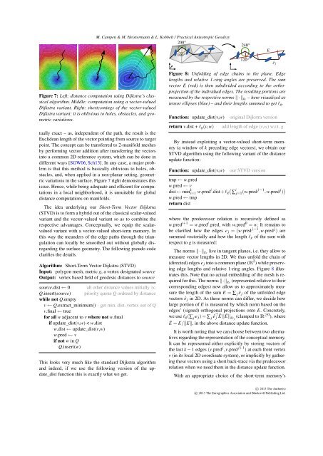
M. Campen & M. Heistermann & L. Kobbelt / Practical Anisotropic Geodesy
200 ◦ 120 ◦
240 ◦ E
100 ◦
e j
ê j
Figure 7: Left: distance computation using Dijkstra’s classical
algorithm. Middle: computation using a vector-valued
Dijkstra variant. Right: shortcomings of the vector-valued
Dijkstra variant: it is oblivious to holes, obstacles, and geometric
variations.
tually exact – as, independent of the path, the result is the
Euclidean length of the vector pointing from source to target
point. The concept can be transferred to 2-manifold meshes
by performing vector addition after transferring the vectors
into a common 2D reference system, which can be done in
different ways [SGW06, Sch13]. In any case, a major problem
is that this method is basically oblivious to holes, obstacles,
and, when applied in a non-planar setting, geometric
variations in the surface. Figure 7 right demonstrates this
issue. Hence, while being adequate and efficient for computations
in a local neighborhood, it is unsuitable for global
distance computations on manifolds.
The idea underlying our Short-Term Vector Dijkstra
(STVD) is to form a hybrid out of the classical scalar-valued
variant and the vector-valued variant so as to combine the
respective advantages. Conceptually, we equip the scalarvalued
variant with a vector-valued short-term memory. In
this way the meanders of the edge paths through the triangulation
can locally be smoothed out without globally disregarding
the surface geometry. The following pseudo code
clarifies the details.
Algorithm: Short-Term Vector Dijkstra (STVD)
Input: polygon mesh, metric g, a vertex designated source
Output: vertex based field of geodesic distances to source
source.dist ← 0 all other distance values initially ∞
Q.insert(source) priority queue Q ordered by distance
while not Q.empty
v ← Q.extract_minimum() get min. dist. vertex out of Q
v.final ← true
for all w adjacent to v where not w.final
if update_dist(v,w) < w.dist
w.dist ← update_dist(v,w)
w.pred ← v
if not w in Q
Q.insert(w)
This looks very much like the standard Dijkstra algorithm
and indeed, if we use the following version of the update_dist
function this is exactly what we get.
Figure 8: Unfolding of edge chains to the plane. Edge
lengths and relative 1-ring angles are preserved. The sum
vector E (red) is then subdivided according to the orthoprojection
of the individual edges. The resulting portions are
measured by the respective norms ‖·‖ ge – here visualized as
tensor ellipses (blue) – and their lengths summed to get l g.
Function: update_dist(v,w)
return v.dist + l g(v,w)
original Dijkstra version
add length of edge (v,w) w.r.t. g
By instead exploiting a vector-valued short-term memory
(a window of k preceding edge vectors), we obtain our
STVD algorithm using the following variant of the distance
update function:
Function: update_dist(v,w)
our STVD version
tmp ← w.pred
w.pred ← v
dist← min k i=1 w.predi .dist+l g
(
∑
i
j=1 (w.pred j−1 ,w.pred j ) )
w.pred ← tmp
return dist
where the predecessor relation is recursively defined as
w.pred i+1 = w.pred i .pred, with w.pred 0 = w. It remains to
be clarified how the edges e j = (w.pred j−1 ,w.pred j ) are
summed vectorially and how the length l g of the sum with
respect to g is measured:
The norms ‖ · ‖ ge live in tangent planes, i.e. they allow to
measure vector lengths in 2D. We thus unfold the chain of
(directed) edges e j into a common plane (R 2 ) while preserving
edge lengths and relative 1-ring angles. Figure 8 illustrates
this. Note that no actual embedding of the mesh is required
for this. The norms ‖·‖ ge (represented relative to their
corresponding edges) now allow us to approximately measure
the length of the sum E = ∑ j ê j of the unfolded edge
vectors ê j in 2D. As these norms can differ, we decide how
large portion of E is measured by which norm based on the
edges’ (signed) orthogonal projections onto E. Concretely,
we use l g(∑ j e j ) = ∑ j ê ⊤ j Ē ‖Ē‖ gê j
(clamped to R ≥0 ), where
Ē = E/‖E‖, in the above distance update function.
It is worth noting that we can choose between two alternatives
regarding the representation of the conceptual memory.
It can be represented either explicitly by storing vectors of
the last k − 1 edges (v.pred j ,v.pred j+1 ) at each front vertex
v (in its local 2D coordinate system), or implicitly by gathering
these vectors using a short back-trace via the predecessor
relation when we need them in the distance update function.
With an appropriate choice of the short-term memory’s
c○ 2013 The Author(s)
c○ 2013 The Eurographics Association and Blackwell Publishing Ltd.