Paper - Computer Graphics and Multimedia - RWTH Aachen ...
Paper - Computer Graphics and Multimedia - RWTH Aachen ...
Paper - Computer Graphics and Multimedia - RWTH Aachen ...

You also want an ePaper? Increase the reach of your titles
YUMPU automatically turns print PDFs into web optimized ePapers that Google loves.
Eurographics Symposium on Geometry Processing 2013<br />
Yaron Lipman <strong>and</strong> Richard Hao Zhang<br />
(Guest Editors)<br />
Volume 32 (2013), Number 5<br />
Practical Anisotropic Geodesy<br />
Marcel Campen Martin Heistermann Leif Kobbelt<br />
<strong>RWTH</strong> <strong>Aachen</strong> University, Germany<br />
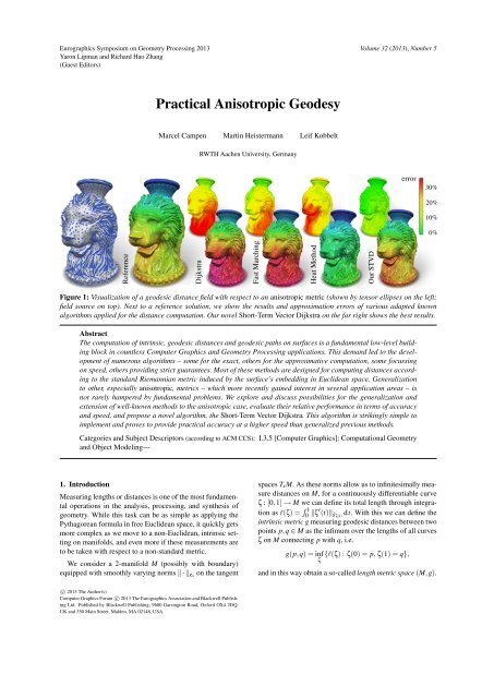
error<br />
30%<br />
20%<br />
10%<br />
0%<br />
Reference<br />
Dijkstra<br />
Fast Marching<br />
Heat Method<br />
Our STVD<br />
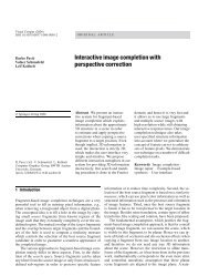
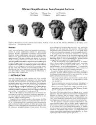
Figure 1: Visualization of a geodesic distance field with respect to an anisotropic metric (shown by tensor ellipses on the left;<br />
field source on top). Next to a reference solution, we show the results <strong>and</strong> approximation errors of various adapted known<br />
algorithms applied for the distance computation. Our novel Short-Term Vector Dijkstra on the far right shows the best results.<br />
Abstract<br />
The computation of intrinsic, geodesic distances <strong>and</strong> geodesic paths on surfaces is a fundamental low-level building<br />
block in countless <strong>Computer</strong> <strong>Graphics</strong> <strong>and</strong> Geometry Processing applications. This dem<strong>and</strong> led to the development<br />
of numerous algorithms – some for the exact, others for the approximative computation, some focussing<br />
on speed, others providing strict guarantees. Most of these methods are designed for computing distances according<br />
to the st<strong>and</strong>ard Riemannian metric induced by the surface’s embedding in Euclidean space. Generalization<br />
to other, especially anisotropic, metrics – which more recently gained interest in several application areas – is<br />
not rarely hampered by fundamental problems. We explore <strong>and</strong> discuss possibilities for the generalization <strong>and</strong><br />
extension of well-known methods to the anisotropic case, evaluate their relative performance in terms of accuracy<br />
<strong>and</strong> speed, <strong>and</strong> propose a novel algorithm, the Short-Term Vector Dijkstra. This algorithm is strikingly simple to<br />
implement <strong>and</strong> proves to provide practical accuracy at a higher speed than generalized previous methods.<br />
Categories <strong>and</strong> Subject Descriptors (according to ACM CCS): I.3.5 [<strong>Computer</strong> <strong>Graphics</strong>]: Computational Geometry<br />
<strong>and</strong> Object Modeling—<br />
1. Introduction<br />
Measuring lengths or distances is one of the most fundamental<br />
operations in the analysis, processing, <strong>and</strong> synthesis of<br />
geometry. While this task can be as simple as applying the<br />
Pythagorean formula in free Euclidean space, it quickly gets<br />
more complex as we move to a non-Euclidean, intrinsic setting<br />
on manifolds, <strong>and</strong> even more if these measurements are<br />
to be taken with respect to a non-st<strong>and</strong>ard metric.<br />
We consider a 2-manifold M (possibly with boundary)<br />
equipped with smoothly varying norms ‖·‖ gx on the tangent<br />
spaces T xM. As these norms allow us to infinitesimally measure<br />
distances on M, for a continuously differentiable curve<br />
ζ : [0,1] → M we can define its total length through integration<br />
as l(ζ) = R 1<br />
0 ‖ζ′ (t)‖ gζ(t) dt. With this we can define the<br />
intrinsic metric g measuring geodesic distances between two<br />
points p,q ∈ M as the infimum over the lengths of all curves<br />
ζ on M connecting p with q, i.e.<br />
g(p,q) = inf{l(ζ) : ζ(0) = p, ζ(1) = q},<br />
ζ<br />
<strong>and</strong> in this way obtain a so-called length metric space (M,g).<br />
c○ 2013 The Author(s)<br />
<strong>Computer</strong> <strong>Graphics</strong> Forum c○ 2013 The Eurographics Association <strong>and</strong> Blackwell Publishing<br />
Ltd. Published by Blackwell Publishing, 9600 Garsington Road, Oxford OX4 2DQ,<br />
UK <strong>and</strong> 350 Main Street, Malden, MA 02148, USA.
M. Campen & M. Heistermann & L. Kobbelt / Practical Anisotropic Geodesy<br />
Note that in the special but common case that ‖ · ‖ gx is<br />
induced by some inner product 〈·,·〉 x on T xM for each x ∈<br />
M, i.e. ‖v‖ gx = √ 〈v,v〉 x, g is a Riemannian metric. If M is<br />
further embedded in Euclidean space – as is the case in most<br />
geometry processing scenarios – the Euclidean dot product<br />
implies a natural inner product via its restriction to T xM. We<br />
call the corresponding norm st<strong>and</strong>ard norm, denoted ‖ · ‖ x,<br />
<strong>and</strong> the induced Riemannian metric st<strong>and</strong>ard metric.<br />
Relative to the st<strong>and</strong>ard metric <strong>and</strong> norm we characterize<br />
a metric g <strong>and</strong> its underlying norm based on their quotient<br />
r(v,x) = ‖v‖ gx /‖v‖ x (for v ≠ 0) as follows:<br />
• If r(v,x) ≡ r(x), i.e. it is independent of v, we call the<br />
metric g isotropic as there is no directional dependency.<br />
• If r(v,x) ≡ r(x) ≢ 1, we call the metric g weighted by the<br />
weight field r(x).<br />
• If r(v,x) ≢ r(x), i.e. there is some directional dependency,<br />
we call the metric g anisotropic.<br />
The value γ(x) = max v r(v,x)/min v r(v,x) defines the local<br />
degree of anisotropy or simply local anisotropy <strong>and</strong><br />
γ = max x γ(x) is the maximum anisotropy.<br />
While the st<strong>and</strong>ard norm realizes the intuitive notion<br />
of geodesic distance <strong>and</strong> is most common in applications,<br />
more general anisotropic norms that incorporate directional<br />
dependencies gained increasing interest in recent years.<br />
Applications range from Meshing [BPC08, CBK12] <strong>and</strong><br />
Segmentation [BPC08, SJC09], over Path Planning [RR90,<br />
LMS99] <strong>and</strong> Shape Matching [SJC09], to (mainly in 3D)<br />
Medical Imaging [PWKB02, PWT05, BCLC09, BC11]. The<br />
anisotropy can be related to principal curvature directions,<br />
terrain steepness, surface vector fields, or MRI diffusion tensors,<br />
to name some examples (cf. Section 3).<br />
Such applications typically operate in a discrete setting,<br />
e.g. on triangle meshes approximating manifolds. Numerous<br />
methods for approximate computation of (mainly isotropic)<br />
distances in such settings have been proposed. Their accuracy<br />
<strong>and</strong> efficiency typically depends on the quality of the<br />
triangulation: intuitively, the “rounder” the individual triangles,<br />
i.e. the closer to equilateral, the better. While working<br />
with rather nice triangulations is quite common in the digital<br />
geometry processing field (leveraged by powerful remeshing<br />
techniques), a problem emerges when anisotropic distances<br />
are dealt with: the notion of “roundness” is metric dependent!<br />
This means a perfectly round triangle which is equilateral<br />
in the st<strong>and</strong>ard metric can be a “cap” or “needle” far<br />
from round when viewed under another, anisotropic metric.<br />
Unfortunately, when naïvely adapting traditional methods<br />
to non-st<strong>and</strong>ard metrics, they expect element roundness<br />
with respect to these metrics, while the meshes typically<br />
used in applications are optimized with respect to the st<strong>and</strong>ard<br />
metric – as often favored by the other processing steps.<br />
Hence, in practice anisotropic distance computations quickly<br />
arrive at inacceptably low accuracy with increasing degree of<br />
anisotropy, as illustrated in Figure 1 for γ = 20.<br />
1.1. Contribution<br />
In this paper we show how (<strong>and</strong> how well) known distance<br />
computation methods proposed for the isotropic st<strong>and</strong>ard<br />
scenario can deal with general metrics, analyze the inherent<br />
issues, <strong>and</strong> discuss the results that can be achieved. For metrics<br />
with a high degree of anisotropy it turns out: typically<br />
either the runtime gets high or the accuracy low. This is problematic<br />
for practical applications in <strong>Computer</strong> <strong>Graphics</strong> <strong>and</strong><br />
Geometry Processing as they rely on distance computations<br />
as a fundamental operation that is used many times.<br />
Improving upon this, we propose Short-Term Vector<br />
Dijkstra: an algorithm that can intuitively be understood as<br />
Dijkstra’s classical shortest path algorithm equipped with a<br />
vector-valued short-term memory. It is fast <strong>and</strong> easy to implement<br />
(hardly more complex than Dijkstra’s method itself)<br />
while providing a practical level of accuracy even for metrics<br />
with a high degree of anisotropy.<br />
2. Related Work<br />
Exact Distances Sophisticated methods using window<br />
propagation or sequence trees [MMP87, CH90, SSK ∗ 05,<br />
XW09] allow for the computation of exact geodesic distances<br />
on triangulated surfaces. Note that this exactness is<br />
with respect to the piecewise-linear surface specified by the<br />
mesh M. In geometry processing scenarios where M itself is<br />
an approximation of a (piecewise) smooth manifold, the expense<br />
of employing such exact algorithms can be futile depending<br />
on the application. This holds even more when we<br />
turn our focus to non-st<strong>and</strong>ard metrics which are also specified<br />
only approximately, e.g. discretely per mesh element.<br />
Graph Approximation Dijkstra’s classical shortest path<br />
algorithm computes shortest paths <strong>and</strong> distances in graphs.<br />
By choosing an appropriate graph <strong>and</strong> suitable edge weights<br />
we can use the corresponding weighted graph distance to approximate<br />
distances on M. In the simplest case this graph is<br />
the 1-skeleton, i.e. the edge graph, of the mesh M, where<br />
the edges are weighted by their length. Higher accuracy,<br />
<strong>and</strong> actually an arbitrary balance between speed <strong>and</strong> accuracy,<br />
can be achieved by constructing a graph with additional<br />
Steiner vertices on M’s edges <strong>and</strong> edges across M’s<br />
faces [Lan99,LMS97,KS00]. The addition of edges between<br />
non-adjacent but nearby vertices [CBK12] allows for faster<br />
computations <strong>and</strong> (at comparable graph size) higher accuracy,<br />
but on the downside no arbitrary balancing is possible.<br />
Consistent Approximation In contrast to these<br />
Dijkstra-based approaches, so-called Fast Marching methods<br />
compute <strong>and</strong> propagate distances not only along edges<br />
of a graph, but also “continuously” across the faces of<br />
a triangle mesh [KS98, SV00, Tsi95]. By appropriate<br />
choices of the per-face propagation rules the approximation<br />
can be made consistent – in the sense that the results<br />
could be driven towards the exact solution by refining the<br />
c○ 2013 The Author(s)<br />
c○ 2013 The Eurographics Association <strong>and</strong> Blackwell Publishing Ltd.
M. Campen & M. Heistermann & L. Kobbelt / Practical Anisotropic Geodesy<br />
mesh. For this, M needs to be an acute triangulation, no<br />
obtuse inner angles are allowed. As this is hardly ever<br />
the case for unstructured meshes in practice, techniques<br />
that add additional virtual edges/triangles to be considered<br />
during the computation have been presented as a<br />
remedy [KS98, SV04, YSS ∗ 12]. Alternative non-linear<br />
propagation rules have been proposed [NK02, TWZZ07],<br />
which can typically increase accuracy in practice – although<br />
at the expense of losing consistency [WDB ∗ 08].<br />
Non-Propagative A very different approach has been<br />
presented by Crane et al. [CWW13]. An approximation to<br />
the intrinsic distance field of a source is computed by means<br />
of solving two global linear systems instead of explicitly<br />
propagating distances from the source over the surface. An<br />
interesting property is leveraged by the information about<br />
sources appearing only on the right h<strong>and</strong> side of the system:<br />
after a pre-factorization, distance fields for different sources<br />
can be computed very efficiently (basically in linear time).<br />
3. Anisotropic Metrics<br />
We consider a discretized setting where, on a triangle mesh<br />
M, an (anisotropic) norm ‖·‖ g is specified in a sampled manner.<br />
The samples can be given per vertex, edge, or face of<br />
M, denoted as ‖ · ‖ gv , ‖ · ‖ ge , or ‖ · ‖ g f<br />
, respectively – where<br />
necessary, we can approximate one form from another via<br />
averaging/interpolation.<br />
Looking at the application scenarios of anisotropic metrics<br />
which appeared in the literature so far, most often Riemannian<br />
metrics are dealt with. In such case, the corresponding<br />
norms can conveniently be expressed through a tensor<br />
field G as ‖v‖ gx = √ v T G xv. Popular examples include:<br />
• Curvature tensor: using the shape operator, tensors<br />
whose eigenvectors are aligned with directions of minimal<br />
<strong>and</strong> maximal curvature of M <strong>and</strong> whose eigenvalues<br />
are related to the magnitude of minimal <strong>and</strong> maximal curvature<br />
can be constructed. Figure 1 exemplarily visualizes<br />
such curvature-related tensors using ellipses.<br />
• Vector field tensor: using the vectors of a tangent vector<br />
field as first eigenvector <strong>and</strong> given two (global) coefficients<br />
to be used as eigenvalues, tensors “aligned” with<br />
the field can be constructed, e.g. to guide geodesic curves<br />
accordingly [CBK12].<br />
• Diffusion tensor: the characteristics of the water diffusion<br />
process in biological tissue can be estimated from<br />
magnetic resonance imaging (MRI) acquisitions <strong>and</strong> be<br />
expressed as a tensor field. Note that this is typically applied<br />
in 3D volumes. While we focus on 2-manifolds here,<br />
we show in Section 6.2 that our novel method is as well<br />
applicable to volumetric meshes or grids.<br />
While such tensor based metrics are widely used, it<br />
bears noting that also more general metrics, based on nonelliptic<br />
norms, are of interest. Examples are terrain steepness<br />
profiles [LMS99], curvature (variation) minimizing metrics<br />
[YSS ∗ 12], or high angular resolution diffusion imaging<br />
(HARDI) metrics [PWT05]. We will hence keep the exposition<br />
general instead of restricting to Riemannian metrics.<br />
4. Generic Adaptation<br />
Before elaborating on the possibilities for individual adaptation<br />
of the available algorithms to a non-st<strong>and</strong>ard norm ‖·‖ g<br />
in Section 5, we discuss a generic way (with certain limitations)<br />
in the following.<br />
4.1. Discrete Metric<br />
Typical implementations of the abovementioned distance<br />
computation algorithms use the vertex coordinates to derive<br />
metric dependent properties like edge lengths, angles, <strong>and</strong><br />
areas. In this way computations implicitly rely on the st<strong>and</strong>ard<br />
metric induced by M’s embedding in Euclidean space.<br />
By not taking any extrinsic vertex coordinates into account,<br />
but instead relying on intrinsic edge lengths, computed<br />
according to ‖ · ‖ g as l g(e) = ‖⃗e‖ ge , most distance<br />
computation algorithms can directly be adapted to nonst<strong>and</strong>ard<br />
norms (an exception is [CBK12], which relies on<br />
(relative) tangent plane orientation information). To that end<br />
one, where required, computes angles <strong>and</strong> areas based on the<br />
intrinsic edge lengths. The intrinsic area A of a triangle with<br />
edge lengths a, b, c can be computed using Heron’s formula<br />
A = 1 4<br />
√<br />
(a + b + c)(−a + b + c)(a − b + c)(a + b − c)<br />
<strong>and</strong> the inner angle α opposing the edge with length a using<br />
the half-angle theorem<br />
√<br />
tan α 2 = (a − b + c)(a + b − c)<br />
(a + b + c)(−a + b + c) .<br />
While being extremely simple, this generic strategy has a<br />
few disadvantages:<br />
Loss of fidelity The metric information is injected solely<br />
via the intrinsic edge lengths, which specifiy the so-called<br />
discrete metric † of the mesh. While such a discrete metric<br />
captures all the information of a (sampled) Riemannian metric,<br />
we inevitably lose fidelity when discretizing a more general<br />
(non-elliptic) norm in this way.<br />
Violation of triangle inequality The computed intrinsic<br />
edge lengths might not fulfill the triangle inequality everywhere<br />
(strictly speaking, they do not form a discrete metric<br />
in this case). We found this to rather be the typical behavior<br />
than the exception, especially for high degrees of anisotropy,<br />
as also described by Kovacs et al. [KMZ11]. For some algorithms<br />
this can be unproblematic, for others (which need<br />
† In literature not related to meshes the term discrete metric by contrast<br />
homonymously refers to a metric which is 0 or 1 everywhere.<br />
c○ 2013 The Author(s)<br />
c○ 2013 The Eurographics Association <strong>and</strong> Blackwell Publishing Ltd.
M. Campen & M. Heistermann & L. Kobbelt / Practical Anisotropic Geodesy<br />
5. Individual Adaptation<br />
We now outline the algorithm specific effects when using<br />
the generic adaptation possibilities presented in the previous<br />
section <strong>and</strong> show options for improved, individual adaptation<br />
where possible.<br />
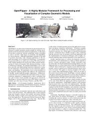
Figure 2: Left: Anisotropic Riemannian metric, visualized<br />
through inverse tensor ellipses (intuitively showing the<br />
“speed profile” of the metric). Middle: Isotropic input mesh.<br />
Right: Corresponding intrinsic Delaunay retriangulation.<br />
to derive angles or areas from these lengths) this is catastrophic.<br />
Edge lengths l ′ (e) fulfilling all triangle inequalities<br />
closest to the desired lengths could in such cases be found<br />
via a suitable inequality-constrained least-squares system:<br />
∑<br />
e<br />
(l ′ (e) − l(e)) 2 → min s.t. l ′ (e i ) ≤ l ′ (e j ) + l ′ (e k ) − ε<br />
for all edge triples e i ,e j ,e k incident to a common face, i.e.<br />
we have three inequality constraints per face.<br />
Low triangulation quality The intrinsic roundness of<br />
the triangles is typically very bad, especially for higher degrees<br />
of anisotropy, i.e. there are angles close to 180 ◦ as well<br />
as angles close to 0 ◦ . For some algorithms this implies a low<br />
accuracy, for others a higher runtime. A remedy can be to<br />
retriangulate the mesh by means of an intrinsic Delaunay<br />
triangulation as detailed in the following.<br />
4.2. Intrinsic Delaunay Triangulation<br />
Using a Delaunay retriangulation algorithm which is based<br />
on an intrinsic discrete metric [FSSB07] we can adjust the<br />
connectivity of the mesh so as to obtain a mesh whose elements<br />
are nice with respect to this intrinsic metric (cf. Figure<br />
2) – to the degree permitted by the given vertex set.<br />
A complete intrinsic remeshing, which not only adjusts the<br />
connectivity but also redistributes vertices, is a theoretical<br />
option that could lead to even better results but would be<br />
rather problematic depending on the application.<br />
While this intrinsic Delaunay Triangulation (iDT) can significantly<br />
improve the distance computation results of several<br />
algorithms, there are some drawbacks, too:<br />
• Numerical inaccuracies can hinder the iDT’s correct execution<br />
<strong>and</strong> termination, thus dem<strong>and</strong> epsilon tweaking,<br />
• The application <strong>and</strong> underlying data structures must support<br />
non-regular meshes [FSSB07] (or the algorithm must<br />
be relaxed to avoid such configurations),<br />
• The input edge lengths must fulfill the triangle inequality<br />
everywhere,<br />
• The worst case runtime complexity is quadratic in the<br />
mesh size.<br />
5.1. Dijkstra<br />
Clearly, the simplest solution to compute approximations to<br />
distances with respect to non-st<strong>and</strong>ard metrics is to apply<br />
Dijkstra’s algorithm, taking the intrinsic edge lengths of the<br />
discrete metric into account. Note that, due to the graph nature<br />
of the algorithm, fulfillment of the triangle inequality is<br />
not required. Unfortunately, the (already in the isotropic case<br />
relatively high) average approximation error increases with<br />
increasing anisotropy, quickly leading to unacceptably low<br />
accuracy. Using the iDT, however, accuracy can be brought<br />
closer to the level of the isotropic case. Figure 3 illustrates<br />
this using the setup from Figure 2 with anisotropy γ = 20.<br />
The Dijkstra-based method of Lanthier [Lan99] which<br />
considers additional vertices <strong>and</strong> edges across faces can be<br />
adapted to the anisotropic case as follows: instead of deriving<br />
the intrinsic lengths of the additional edges from the discrete<br />
metric, we calculate the length of an edge across face<br />
f directly using ‖ · ‖ g f<br />
. This allows for higher fidelity in the<br />
case of non-Riemannian metrics. Figure 4 illustrates the behavior<br />
for increasing numbers of added vertices <strong>and</strong> edges.<br />
In the Dijkstra-based method of Campen et al. [CBK12]<br />
one can similarly compute intrinsic lengths for the additional<br />
edges directly based on the norms ‖ · ‖ ge instead of relying<br />
on the discrete metric approach, as described by the authors.<br />
5.2. Fast Marching<br />
The Fast Marching approach [KS98] can be applied in the<br />
case of a non-st<strong>and</strong>ard metric by relying on the corresponding<br />
discrete metric (which must fulfill the triangle inequality<br />
everywhere as we need to derive, e.g., angles from it). The<br />
general problem is that in this metric the number of obtuse<br />
triangles is often enormous, requiring the consideration of a<br />
vast number of virtual edges. An iDT can be used to avoid<br />
this – but has its own abovementioned shortcomings. Figure<br />
5 illustrates the qualities of these options. Another option<br />
is to deal with the inaccuracies due to obtuse angles using<br />
recursive improvement techniques [KSC ∗ 07]; however, this<br />
means losing consistency <strong>and</strong> convergence properties.<br />
Sethian <strong>and</strong> Vladimirsky [SV04] proposed a more general<br />
Ordered Upwind method (OUM) which is already specifically<br />
designed for non-st<strong>and</strong>ard metrics. It is able to consistently<br />
deal with arbitrary anisotropy, i.e. one, in theory,<br />
has the possibility to arbitrarily increase accuracy through<br />
mesh refinement. In comparison to the other discussed algorithms,<br />
the implementation is probably the most complex<br />
one <strong>and</strong> runtime <strong>and</strong> memory consumption is relatively<br />
c○ 2013 The Author(s)<br />
c○ 2013 The Eurographics Association <strong>and</strong> Blackwell Publishing Ltd.
M. Campen & M. Heistermann & L. Kobbelt / Practical Anisotropic Geodesy<br />
Reference Dijkstra Dijkstra iDT<br />
FM w/o virt. edges FM FM iDT<br />
Figure 3: Anisotropic distance field (up to a fixed maximum<br />
distance, so as to enhance clarity). Left: Highly accurate<br />
reference solution. Middle: Dijkstra result on an isotropic<br />
mesh. Right: Dijkstra result computed on the iDT.<br />
5 Steiner 10 Steiner 20 Steiner<br />
Figure 5: Fast Marching distance field based on the discrete<br />
metric. Left: without virtual edges. Middle: with 13k virtual<br />
edges. Right: on the iDT, where only 6k virtual edges are<br />
necessary.<br />
Heat Heat iDT tuned time step<br />
Figure 4: Lanthier’s method’s distance field (on the isotropic<br />
mesh). Left: computed with 5 Steiner vertices per<br />
edge. Middle: 10 Steiner vertices. Right: 20 Steiner vertices.<br />
high (cf. Section 7). A main factor is that, in addition to<br />
the actual anisotropic distance propagation, as an ingredient<br />
isotropic distances from every single vertex of the mesh<br />
to all of its neighbors within a radius of ‖e max‖γ need to be<br />
computed. Here e max is the longest edge of the mesh <strong>and</strong><br />
γ the anisotropy, i.e. the radius can become quite large for<br />
high anisotropies. While simple extrinsic distances can be<br />
used for efficiency, higher accuracy on non-planar meshes is<br />
achieved by computing intrinsic isotropic distances.<br />
It is worth noting that, while other<br />
OUM<br />
methods typically overestimate distances,<br />
OUM can also heavily underestimate<br />
distances, as can be seen<br />
when comparing the inset figure to the<br />
reference solution. This is due to the<br />
fact that distances are propagated over<br />
virtual triangles that span a long distance<br />
across the mesh. While the norm potentially varies on<br />
the mesh under these virtual triangles, the propagation across<br />
them is computed atomically using only the norm at one end<br />
point, easily allowing for too long as well as too short results.<br />
5.3. Heat Method<br />
Just like the other algorithms discussed so far, the heat<br />
method [CWW13] can be adapted to non-st<strong>and</strong>ard metrics<br />
by formulating it in terms of the discrete metric, i.e. based<br />
on the intrinsic edge lengths. This amounts to calculating the<br />
cotangent weights, element areas, <strong>and</strong> divergence values involved<br />
in the Laplacian <strong>and</strong> the Poisson system accordingly.<br />
Figure 6: Heat Method distance field based on the discrete<br />
metric. Left: computed on the isotropic mesh. Middle: computed<br />
on the iDT. Right: computed on the isotropic mesh but<br />
with individually tuned heat integration time step.<br />
Unless the anisotropy is very moderate, the low intrinsic<br />
element roundness, however, does negatively affect robustness.<br />
The resulting distance fields then often show distortions<br />
<strong>and</strong> degeneracies like local minima. We observed that<br />
improved results can be achieved by individually tuning the<br />
heat integration time step instead of using the st<strong>and</strong>ard c = 5<br />
proposed in the original publication, but found no general<br />
rule for a good automatic choice. Again, an iDT can be an<br />
option to remedy these problems (cf. Figure 6).<br />
6. Short-Term Vector Dijkstra<br />
We now present a novel method for the approximate computation<br />
of distances with respect to arbitrary metrics. In order<br />
to develop an intuitive underst<strong>and</strong>ing of the underlying<br />
principle, let us consider Dijkstra’s classical algorithm again.<br />
Due to its graph nature, the distance approximations resulting<br />
from this algorithm are the lengths of edge paths that<br />
me<strong>and</strong>er over the surface (cf. Figure 7 left) – not the lengths<br />
of true geodesic paths. They are thus rather inaccurate <strong>and</strong><br />
also very triangulation dependent.<br />
Instead of first measuring lengths of edges <strong>and</strong> then<br />
(scalarly) summing these, an interesting alternative is to first<br />
(vectorially) sum edges <strong>and</strong> then measure the length of the<br />
sum. This vector-valued Dijkstra algorithm has been employed<br />
by Schmidt et al. [SGW06] to obtain geodesic distances<br />
for the purpose of local surface parameterization. Figure<br />
7 illustrates the principle in the plane. In this planar case<br />
<strong>and</strong> with the st<strong>and</strong>ard metric the resulting distances are acc○<br />
2013 The Author(s)<br />
c○ 2013 The Eurographics Association <strong>and</strong> Blackwell Publishing Ltd.
M. Campen & M. Heistermann & L. Kobbelt / Practical Anisotropic Geodesy<br />
200 ◦ 120 ◦<br />
240 ◦ E<br />
100 ◦<br />
e j<br />
ê j<br />
Figure 7: Left: distance computation using Dijkstra’s classical<br />
algorithm. Middle: computation using a vector-valued<br />
Dijkstra variant. Right: shortcomings of the vector-valued<br />
Dijkstra variant: it is oblivious to holes, obstacles, <strong>and</strong> geometric<br />
variations.<br />
tually exact – as, independent of the path, the result is the<br />
Euclidean length of the vector pointing from source to target<br />
point. The concept can be transferred to 2-manifold meshes<br />
by performing vector addition after transferring the vectors<br />
into a common 2D reference system, which can be done in<br />
different ways [SGW06, Sch13]. In any case, a major problem<br />
is that this method is basically oblivious to holes, obstacles,<br />
<strong>and</strong>, when applied in a non-planar setting, geometric<br />
variations in the surface. Figure 7 right demonstrates this<br />
issue. Hence, while being adequate <strong>and</strong> efficient for computations<br />
in a local neighborhood, it is unsuitable for global<br />
distance computations on manifolds.<br />
The idea underlying our Short-Term Vector Dijkstra<br />
(STVD) is to form a hybrid out of the classical scalar-valued<br />
variant <strong>and</strong> the vector-valued variant so as to combine the<br />
respective advantages. Conceptually, we equip the scalarvalued<br />
variant with a vector-valued short-term memory. In<br />
this way the me<strong>and</strong>ers of the edge paths through the triangulation<br />
can locally be smoothed out without globally disregarding<br />
the surface geometry. The following pseudo code<br />
clarifies the details.<br />
Algorithm: Short-Term Vector Dijkstra (STVD)<br />
Input: polygon mesh, metric g, a vertex designated source<br />
Output: vertex based field of geodesic distances to source<br />
source.dist ← 0 all other distance values initially ∞<br />
Q.insert(source) priority queue Q ordered by distance<br />
while not Q.empty<br />
v ← Q.extract_minimum() get min. dist. vertex out of Q<br />
v.final ← true<br />
for all w adjacent to v where not w.final<br />
if update_dist(v,w) < w.dist<br />
w.dist ← update_dist(v,w)<br />
w.pred ← v<br />
if not w in Q<br />
Q.insert(w)<br />
This looks very much like the st<strong>and</strong>ard Dijkstra algorithm<br />
<strong>and</strong> indeed, if we use the following version of the update_dist<br />
function this is exactly what we get.<br />
Figure 8: Unfolding of edge chains to the plane. Edge<br />
lengths <strong>and</strong> relative 1-ring angles are preserved. The sum<br />
vector E (red) is then subdivided according to the orthoprojection<br />
of the individual edges. The resulting portions are<br />
measured by the respective norms ‖·‖ ge – here visualized as<br />
tensor ellipses (blue) – <strong>and</strong> their lengths summed to get l g.<br />
Function: update_dist(v,w)<br />
return v.dist + l g(v,w)<br />
original Dijkstra version<br />
add length of edge (v,w) w.r.t. g<br />
By instead exploiting a vector-valued short-term memory<br />
(a window of k preceding edge vectors), we obtain our<br />
STVD algorithm using the following variant of the distance<br />
update function:<br />
Function: update_dist(v,w)<br />
our STVD version<br />
tmp ← w.pred<br />
w.pred ← v<br />
dist← min k i=1 w.predi .dist+l g<br />
(<br />
∑<br />
i<br />
j=1 (w.pred j−1 ,w.pred j ) )<br />
w.pred ← tmp<br />
return dist<br />
where the predecessor relation is recursively defined as<br />
w.pred i+1 = w.pred i .pred, with w.pred 0 = w. It remains to<br />
be clarified how the edges e j = (w.pred j−1 ,w.pred j ) are<br />
summed vectorially <strong>and</strong> how the length l g of the sum with<br />
respect to g is measured:<br />
The norms ‖ · ‖ ge live in tangent planes, i.e. they allow to<br />
measure vector lengths in 2D. We thus unfold the chain of<br />
(directed) edges e j into a common plane (R 2 ) while preserving<br />
edge lengths <strong>and</strong> relative 1-ring angles. Figure 8 illustrates<br />
this. Note that no actual embedding of the mesh is required<br />
for this. The norms ‖·‖ ge (represented relative to their<br />
corresponding edges) now allow us to approximately measure<br />
the length of the sum E = ∑ j ê j of the unfolded edge<br />
vectors ê j in 2D. As these norms can differ, we decide how<br />
large portion of E is measured by which norm based on the<br />
edges’ (signed) orthogonal projections onto E. Concretely,<br />
we use l g(∑ j e j ) = ∑ j ê ⊤ j Ē ‖Ē‖ gê j<br />
(clamped to R ≥0 ), where<br />
Ē = E/‖E‖, in the above distance update function.<br />
It is worth noting that we can choose between two alternatives<br />
regarding the representation of the conceptual memory.<br />
It can be represented either explicitly by storing vectors of<br />
the last k − 1 edges (v.pred j ,v.pred j+1 ) at each front vertex<br />
v (in its local 2D coordinate system), or implicitly by gathering<br />
these vectors using a short back-trace via the predecessor<br />
relation when we need them in the distance update function.<br />
With an appropriate choice of the short-term memory’s<br />
c○ 2013 The Author(s)<br />
c○ 2013 The Eurographics Association <strong>and</strong> Blackwell Publishing Ltd.
M. Campen & M. Heistermann & L. Kobbelt / Practical Anisotropic Geodesy<br />
depth k, the accuracy of the results is<br />
immensely improved. The inset illustrates<br />
this for k = 10 (detailed quantitative<br />
results are provided in Section 7).<br />
Despite the lack of smoothness in some<br />
regions, the result is closer to the reference<br />
than the alternatives from Section<br />
5 (except Figure 4 middle, right).<br />
STVD<br />
Note that for k = 1 STVD is equivalent to Dijkstra’s classical<br />
algorithm (generally overestimating distances), while<br />
for k → ∞ it becomes an all vector-valued variant (which<br />
tends to underestimate unless the surface is developable <strong>and</strong><br />
free of holes). This can also be observed in the following<br />
histograms which show the signed relative error distribution<br />
over all vertices of all examples from Section 7 (for γ = 10):<br />
80%<br />
40%<br />
0%<br />
– 40%<br />
k = 1 k = 2 k = 4 k = 6 k = 8 k = 10<br />
In a previous method [CBK12] also edge chains up to a<br />
length k were considered for distance computations. A fundamental<br />
difference is that the mesh graph is extended with<br />
additional edges, increasing their total number by about two<br />
orders of magnitude in practice. This has direct performance<br />
consequences as the runtime of Dijkstra’s algorithm depends<br />
on the number of edges. By contrast, our method performs<br />
just one distance value update computation per original input<br />
edge, just like the st<strong>and</strong>ard Dijkstra algorithm. This difference<br />
is due to not constructing (in advance) all possible<br />
edge chains of length ≤ k, but implicitly (on dem<strong>and</strong>) only<br />
those which are actually proceeding in the direction of the<br />
propagating front. Further differences are that, due to the<br />
employed discrete exponential map, this previous method relies<br />
on an embedding of the surface, <strong>and</strong> the construction is<br />
specifically tailored to a direction field based metric.<br />
6.1. Speed vs. Accuracy<br />
Some of the discussed algorithms allow to trade speed for accuracy<br />
at the user’s discretion. By using a higher number of<br />
Steiner vertices in the edge-subdivision approach [Lan99],<br />
or by refining the input triangle mesh using some steps of<br />
1-to-4 splits prior to the application of the Ordered Upwind<br />
method [SV04] (or, in the case of a Riemannian metric,<br />
also the Fast Marching adaptation) higher accuracy can be<br />
achieved – at the cost of quickly increasing runtime. Note<br />
that such property is not to be taken for granted: for instance<br />
the accuracy of distance computations using Dijkstra’s algorithm<br />
does not generally increase under mesh refinement.<br />
We empirically observed that such property can also be<br />
established for our STVD. To this end we need to achieve<br />
two seemingly contradicting goals: k needs to be increased<br />
so as to increase the angular resolution of the distance propagation,<br />
while the lengths of the used vector sums need to<br />
be decreased so as to reduce the approximation errors of the<br />
unfolding-based measurement. We can achieve both by refining<br />
the mesh using 1-to-4 splits (reducing edge lengths by<br />
a factor of 2) while increasing k by a factor < 2. The following<br />
table shows the decreasing mean error for increasing<br />
levels of refinement on three exemplary models (γ = 20):<br />
Level k ELKTOY GARGOYLE ROCKERARM<br />
0 7 9.8% 25.7% 15.3%<br />
1 10 5.1% 13.4% 11.6%<br />
2 14 2.5% 8.2% 6.5%<br />
3 20 1.5% 4.3% 3.9%<br />
More interesting than this possibility, however, we deem<br />
that, even in the case of strong anisotropy, STVD achieves<br />
reasonable, relatively good results already on unrefined<br />
meshes of resolutions typically encountered in the <strong>Computer</strong><br />
<strong>Graphics</strong> <strong>and</strong> Geometry Processing field (cf. Section 7).<br />
6.2. Genericity<br />
Polygonal Meshes It is worth noting that STVD does not<br />
rely on the property that M is a triangle mesh, i.e. it can also<br />
be applied to general polygonal meshes. Many other methods<br />
are designed specifically for triangle meshes <strong>and</strong> would<br />
need to be adapted – or the polygon mesh be triangulated.<br />
3D Meshes While our focus here is on 2-manifold surface<br />
meshes, an interesting fact about STVD is that it can directly<br />
be applied also to volumetric meshes in R 3 – whether<br />
they consist of tetrahedral, hexahedral, or general polyhedral<br />
cells. We simply skip the edge vector unfolding to the<br />
plane <strong>and</strong> sum the 3D edge vectors directly (cf. Figure 9).<br />
While also other methods can potentially be generalized to<br />
this setting, this is less trivial. Challenges lie in the correct<br />
determination of virtual simplices for the OUM or FMM,<br />
establishing an intrinsic Delaunay tetrahedralization or fixing<br />
violated tetrahedra inequalities, or in h<strong>and</strong>ling the large<br />
number of additional edges, which in the case of straight-<br />
Dijkstra STVD Dijkstra STVD<br />
Figure 9: Volumetric distance fields computed in a hexahedra<br />
<strong>and</strong> a tetrahedra mesh (sliced open to expose the interior).<br />
The constant Riemannian metrics used (depicted by<br />
ellipsoids next to the models) have an anisotropy of 12. Just<br />
like in the surface mesh case, Dijkstra’s algorithm heavily<br />
overestimates distances, especially in vertical direction<br />
where true distances are shorter due to the anisotropy.<br />
c○ 2013 The Author(s)<br />
c○ 2013 The Eurographics Association <strong>and</strong> Blackwell Publishing Ltd.
M. Campen & M. Heistermann & L. Kobbelt / Practical Anisotropic Geodesy<br />
forward generalization of Lanthier’s concept to 3D grows<br />
quartically with the number of Steiner vertices per edge.<br />
7. Results<br />
In the previous sections we have discussed the qualitative<br />
differences of the approaches that are available for the computation<br />
of anisotropic distances. In order to get a quantitative<br />
underst<strong>and</strong>ing for the accuracy <strong>and</strong> runtime performance<br />
of all these options, we implemented all variants <strong>and</strong> performed<br />
extensive experiments using various kinds of input<br />
meshes (cf. Figure 10, 9K-183K triangles), metrics (vector<br />
field based as well as curvature tensor based), anisotropies<br />
(uniform as well as varying γ(x)), <strong>and</strong> algorithm parameters.<br />
The reference solutions we compare against have been<br />
computed using the edge-subdivision method of Lanthier<br />
[Lan99] with 200 Steiner vertices per edge (<strong>and</strong> runtimes<br />
of up to several hours for a single distance field). In this setting<br />
for every single triangle there are more than 120,000<br />
virtual edges crossing it, resulting in a highly accurate approximation<br />
of the true distances. We show the results using<br />
error-over-runtime plots in Figure 11 (<strong>and</strong> using error histograms<br />
in the supplemental material). Intuitively, the closer<br />
a method lies to the bottom left, the better – as this means<br />
that a low error (high accuracy) is achieved in a short time.<br />
These plots further allow to quickly see what other options<br />
apart from the “best one” are available, e.g. how much more<br />
accuracy can be achieved by spending how much more time.<br />
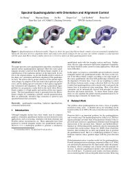
Regarding our STVD algorithm, we see that it lies in the<br />
bottom left region across the different levels of anisotropy,<br />
i.e. it achieves good results in short time when compared to<br />
the other options – especially for higher anisotropies. Good<br />
st<strong>and</strong>ard values for k can also be read from these plots: from<br />
around 5 for low anisotropy to around 10 for anisotropy 50.<br />
Note that such high anisotropy is not only of theoretical interest,<br />
e.g. anisotropies of 30+ have been used in [CBK12].<br />
For lower anisotropies, the Fast Marching method applied<br />
to the intrinsic Delaunay triangulation of a subdivided version<br />
of the input mesh is very competitive. Note that this<br />
strategy requires several steps of preprocessing: 1) mesh<br />
subdivision, 2) discrete metric computation, 3) reestablishing<br />
triangle inequality fulfillment, <strong>and</strong> 4) iDT construction.<br />
This also implies the drawbacks discussed in Sections 4.1<br />
<strong>and</strong> 4.2 <strong>and</strong> can take a considerable amount of (possibly<br />
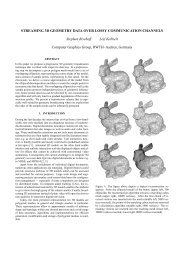
Figure 10: Models used for the evaluation, depicted with example<br />
fields. (From the AIM@SHAPE repository, the Imagebased<br />
3D Models Archive, Télécom Paris, or created using<br />
Cosmic Blobs R○ by Dassault Systèmes Solidworks Corp.)<br />
amortizable) time. By contrast, STVD operates directly on<br />
the input mesh without the need for any preprocessing <strong>and</strong><br />
without implying additional complexity.<br />
When a higher level of accuracy is required <strong>and</strong> more<br />
time is available, the edge subdivision method of Lanthier<br />
[Lan99] proves to consistently provide a good option.<br />
In isotropic scenarios the advantage of STVD over, e.g.,<br />
Fast Marching or the Heat Method diminishes. However,<br />
we observed that it is typically still very significant when<br />
dealing with meshes with badly shaped elements. This is illustrated<br />
here on an example mesh (γ = 1), where the error<br />
(w.r.t. exact geodesic distances [SSK ∗ 05]) is visualized:<br />
12%<br />
9%<br />
6%<br />
3%<br />
0%<br />
8. Conclusion<br />
Dijkstra FM Heat<br />
(tuned time step)<br />
STVD<br />
(k =5)<br />
We have explored <strong>and</strong> discussed numerous options for<br />
the computation of distance fields with respect to general<br />
anisotropic metrics, based on generic as well as specific<br />
adaptations of known algorithms. We compared all these in<br />
terms of their accuracy <strong>and</strong> runtime performance <strong>and</strong> enriched<br />
this zoo of methods with our Short-Term Vector Dijkstra.<br />
Despite its simplicity, this method proved to provide<br />
a very interesting novel option, allowing to quickly compute<br />
results with practical accuracy without the need for complex<br />
optimization or costly preprocessing.<br />
In the future we would like to explore ways to enhance<br />
the smoothness of the results. Possibilities could be the use<br />
of averaging schemes during propagation [Sch13] or of a<br />
kind of “gradually fading memory” instead of a hard limit k.<br />
The use of a locally varying k (based on local feature size,<br />
anisotropy, mesh density) is another interesting direction.<br />
Acknowledgements Funding for this work was provided by<br />
the DFG Cluster of Excellence UMIC, grant DFG EXC 89.<br />
References<br />
[BC11] BENMANSOUR F., COHEN L. D.: Tubular structure segmentation<br />
based on minimal path method <strong>and</strong> anisotropic enhancement.<br />
Int. J. of <strong>Computer</strong> Vision 92, 2 (2011), 192–210.<br />
[BCLC09] BENMANSOUR F., COHEN L. D., LAW M. W. K.,<br />
CHUNG A. C. S.: Tubular anisotropy for 2d vessel segmentation.<br />
In CVPR (2009), pp. 2286–2293.<br />
[BPC08] BOUGLEUX S., PEYRÉ G., COHEN L. D.: Anisotropic<br />
Geodesics for Perceptual Grouping <strong>and</strong> Domain Meshing. In<br />
ECCV (2008), vol. 5303, pp. 129—-142.<br />
[CBK12] CAMPEN M., BOMMES D., KOBBELT L.: Dual Loops<br />
Meshing: Quality Quad Layouts on Manifolds. ACM Transactions<br />
on <strong>Graphics</strong> 31, 4 (2012), 110:1—-110:11.<br />
c○ 2013 The Author(s)<br />
c○ 2013 The Eurographics Association <strong>and</strong> Blackwell Publishing Ltd.
M. Campen & M. Heistermann & L. Kobbelt / Practical Anisotropic Geodesy<br />
γ = 5 γ = 10 γ = 20 γ = 50<br />
Figure 11: Error-over-runtime plots of the results for various degrees of anisotropy (γ). Shown is the mean rel. abs. error<br />
(computed over all vertices) on the vertical axis, <strong>and</strong> the summed runtime (sec.) for the computation of a complete distance field<br />
per input test case (14 mesh/metric combinations). Mesh subdivision (1-to-4 split) levels are indicated by I <strong>and</strong> II; numbers<br />
indicate the STVD parameter k or the number of edge Steiner vertices, respectively. Preprocessing time (shown by dashed bars)<br />
includes triangle inequality fixing <strong>and</strong> (where applicable) subdivision <strong>and</strong> iDT. For the Heat method the first segment of the bar<br />
additionally indicates the time for setup <strong>and</strong> pre-factorization of the employed linear systems. Violated triangle inequalities have<br />
been fixed 1) for the heat method as described in Section 4.1 using Ipopt; 2) for the FMM using a simpler (not least-squares<br />
optimal) strategy of iteratively adjusting individual triangles, as on the subdivided meshes the solver takes unacceptably long.<br />
[CH90] CHEN J., HAN Y.: Shortest Paths on a Polyhedron. In<br />
Proc. Symp. Comp. Geom. (1990), pp. 360–369.<br />
[CWW13] CRANE K., WEISCHEDEL C., WARDETZKY M.:<br />
Geodesics in Heat. ACM Transactions on <strong>Graphics</strong> (2013).<br />
[FSSB07] FISHER M., SPRINGBORN B., SCHRÖDER P.,<br />
BOBENKO A. I.: An algorithm for the construction of intrinsic<br />
delaunay triangulations with applications to digital geometry<br />
processing. Computing 81, 2-3 (2007), 199–213.<br />
[KMZ11] KOVACS D., MYLES A., ZORIN D.: Anisotropic quadrangulation.<br />
Comp. Aided Geom. Design 28, 8 (2011), 449–462.<br />
[KS98] KIMMEL R., SETHIAN J. A.: Computing geodesic paths<br />
on manifolds. Proc. Natl. Acad. Sci. 95, 15 (1998), 8431–8435.<br />
[KS00] KANAI T., SUZUKI H.: Approximate Shortest Path on<br />
Polyhedral Surface Based on Selective Refinement of the Discrete<br />
Graph <strong>and</strong> its Applications. In Geometric Modeling <strong>and</strong><br />
Processing (2000), IEEE Comput. Soc, pp. 241–250.<br />
[KSC ∗ 07] KONUKOGLU E., SERMESANT M., CLATZ O.,<br />
PEYRAT J.-M., DELINGETTE H., AYACHE N.: A recursive<br />
anisotropic fast marching approach to reaction diffusion equation:<br />
Application to tumor growth modeling. In IPMI (2007),<br />
pp. 687–699.<br />
[Lan99] LANTHIER M.: Shortest Path Problems on Polyhedral<br />
Surfaces. PhD thesis, School of <strong>Computer</strong> Science, Carleton University,<br />
1999.<br />
[LMS97] LANTHIER M., MAHESHWARI A., SACK J.-R.: Approximating<br />
weighted shortest paths on polyhedral surfaces.<br />
Proc. Symp. Comp. Geom. (SCG ’97) (1997), 274–283.<br />
[LMS99] LANTHIER M., MAHESHWARI A., SACK J.-R.: Shortest<br />
Anisotropic Paths on Terrains. ICAL 26 (1999), 523—-533.<br />
[MMP87] MITCHELL J. S., MOUNT D. M., PAPADIMITRIOU<br />
C. H.: The Discrete Geodesic Problem. SIAM Journal on Computing<br />
16, 4 (1987), 647–668.<br />
[NK02] NOVOTNI M., KLEIN R.: Computing Geodesic Distances<br />
on Triangular Meshes. In WSCG (2002),UniversitätBonn.<br />
[PWKB02] PARKER G. J. M., WHEELER-KINGSHOTT C.<br />
A. M., BARKER G. J.: Estimating distributed anatomical brain<br />
connectivity using fast marching methods <strong>and</strong> diffusion tensor<br />
imaging. IEEE Trans. Med. Imaging 21, 5 (2002), 505–512.<br />
[PWT05]<br />
PICHON E., WESTIN C.-F., TANNENBAUM A. R.: A<br />
Hamilton-Jacobi-Bellman approach to high angular resolution<br />
diffusion tractography. Medical image computing <strong>and</strong> computerassisted<br />
intervention 8, Pt 1 (Jan. 2005), 180–7.<br />
[RR90] ROWE N. C., ROSS R. S.: Optimal grid-free path planning<br />
across arbitrarily-contoured terrain with anisotropic friction<br />
<strong>and</strong> gravity effects. IEEE Trans. Robot. Autom (1990).<br />
[Sch13] SCHMIDT R.: Stroke parameterization. Comp. Graph.<br />
Forum 32, 2 (2013).<br />
[SGW06] SCHMIDT R., GRIMM C., WYVILL B.: Interactive Decal<br />
Compositing with Discrete Exponential Maps. ACM Transactions<br />
on <strong>Graphics</strong> 25, 3 (2006), 605—-613.<br />
[SJC09] SEONG J.-K., JEONG W.-K., COHEN E.: Curvaturebased<br />
anisotropic geodesic distance computation for parametric<br />
<strong>and</strong> implicit surfaces. The Visual <strong>Computer</strong> 25, 8 (Apr. 2009),<br />
743–755.<br />
[SSK ∗ 05] SURAZHSKY V., SURAZHSKY T., KIRSANOV D.,<br />
GORTLER S. J., HOPPE H.: Fast exact <strong>and</strong> approximate<br />
geodesics on meshes. In SIGGRAPH (2005), vol. 24.<br />
[SV00] SETHIAN J. A., VLADIMIRSKY A.: Fast methods for the<br />
Eikonal <strong>and</strong> related Hamilton- Jacobi equations on unstructured<br />
meshes. Proc. Nat. Acad. Sci. 97, 11 (2000), 5699–703.<br />
[SV04] SETHIAN J. A., VLADIMIRSKY A.: Ordered Upwind<br />
Methods for Static Hamilton-Jacobi Equations: Theory <strong>and</strong> Algorithms.<br />
SIAM J. Num. Anal. 41, 1 (2004), 325–363.<br />
[Tsi95] TSITSIKLIS J. N.: Globally Optimal Trajectories. IEEE<br />
Transactions on Automatic Control 40, 9 (1995), 1528–1538.<br />
[TWZZ07] TANG J., WU G.-S., ZHANG F.-Y., ZHANG M.-M.:<br />
Fast approximate geodesic paths on triangle mesh. International<br />
Journal of Automation <strong>and</strong> Computing 4, 1 (Jan. 2007), 8–13.<br />
[WDB ∗ 08] WEBER O., DEVIR Y. S., BRONSTEIN A. M.,<br />
BRONSTEIN M. M., KIMMEL R.: Parallel algorithms for approximation<br />
of distance maps on parametric surfaces. ACM<br />
Transactions on <strong>Graphics</strong> 27, 4 (2008), 104:1—-104:16.<br />
[XW09] XIN S.-Q., WANG G.-J.: Improving Chen <strong>and</strong> Han’s<br />
algorithm on the discrete geodesic problem. ACM Trans. Graph.<br />
28, 4 (2009), 104:1–104:8.<br />
[YSS ∗ 12] YOO S. W., SEONG J.-K., SUNG M.-H., SHIN S. Y.,<br />
COHEN E.: A triangulation-invariant method for anisotropic<br />
geodesic map computation on surface meshes. IEEE Trans. Vis.<br />
Comput. Graph. 18, 10 (2012), 1664–1677.<br />
c○ 2013 The Author(s)<br />
c○ 2013 The Eurographics Association <strong>and</strong> Blackwell Publishing Ltd.