HP 33120A User's Guide
HP 33120A User's Guide
HP 33120A User's Guide

You also want an ePaper? Increase the reach of your titles
YUMPU automatically turns print PDFs into web optimized ePapers that Google loves.
7<br />
7<br />
Tutorial
Tutorial<br />
The <strong>HP</strong> <strong>33120A</strong> is capable of producing a variety of signal waveshapes.<br />
In order to achieve the greatest performance from the function generator,<br />
it may be helpful if you learn more about the internal operations of the<br />
instrument. This chapter describes basic signal generation concepts and<br />
gives specific details on the internal operations of the function generator.<br />
• Direct Digital Synthesis, starting on page 273<br />
• Signal Imperfections, starting on page 276<br />
• Creating Arbitrary Waveforms, starting on page 278<br />
• Output Amplitude Control, starting on page 280<br />
• Floating Signal Generators, on page 282<br />
• Attributes of AC Signals, starting on page 283<br />
• Modulation, starting on page 287<br />
You can use an arbitrary waveform generator in a variety of applications<br />
where it might be otherwise difficult or impossible to generate complex<br />
output waveforms. With an arbitrary waveform generator, signal<br />
imperfections such as rise time, ringing, glitches, noise, and random<br />
timing variations can be easily simulated in a controlled manner.<br />
Physics, chemistry, biomedicine, electronics, mechanics, and other fields<br />
can benefit from the versatility of an arbitrary waveform generator.<br />
Wherever things vibrate, pump, pulse, bubble, burst, or change with<br />
time in any way, there are possible applications — limited only by your<br />
ability to provide waveform data.<br />
The <strong>HP</strong> 34811A BenchLink/Arb Waveform Generation Software<br />
for Microsoft® Windows TM is designed to make it easy to create<br />
and output arbitrary waveforms for the <strong>HP</strong> <strong>33120A</strong>.<br />
272
Chapter 7 Tutorial<br />
Direct Digital Synthesis<br />
Direct Digital Synthesis<br />
Digital signal processing methods are used in many everyday applications.<br />
Whether it is a digital audio compact disc player, an electronic<br />
synthesized piano, or a voice-synthesized telephone message system,<br />
it is obvious that complex waveforms can be easily created or<br />
reproduced using digital signal generation methods.<br />
The <strong>HP</strong> <strong>33120A</strong> uses a signal-generation technique called direct digital<br />
synthesis or DDS. The basic principle behind DDS is not unlike an audio<br />
compact disc. As shown below for digital audio, a stream of digital data<br />
representing the sampled analog signal shape is sequentially addressed<br />
from a disc. This data is applied to the digital port of a digital-to-analog<br />
converter (DAC) which is clocked at a constant rate. The digital data is<br />
then converted into a series of voltage steps approximating the original<br />
analog signal shape. After filtering the voltage steps, the original analog<br />
waveshape will be recovered. The incoming data can be of any arbitrary<br />
shape, as long as it matches the requirements of the particular DAC<br />
(16 bits for digital audio players).<br />
Anti-Alias Filter<br />
Data<br />
D-to-A<br />
Converter<br />
A<br />
7<br />
273
Chapter 7 Tutorial<br />
Direct Digital Synthesis<br />
Direct Digital<br />
Synthesis<br />
(continued)<br />
A direct digital synthesis (DDS) signal generator differs from a digital<br />
audio player because of its very precise control of the data stream input<br />
to the DAC. In a DDS system, the amplitude values for one complete<br />
cycle of the output waveshape are stored sequentially in random access<br />
memory (RAM) as shown in the figure below. As RAM addresses are<br />
changed, the DAC converts the waveshape data into a voltage waveform<br />
(whose data values are loaded in RAM). The frequency of the voltage<br />
waveform is proportional to the rate at which the RAM addresses<br />
are changed.<br />
The <strong>HP</strong> <strong>33120A</strong> represents amplitude values by 4,096 discrete voltage<br />
levels (or 12-bit vertical resolution). Waveforms may contain between<br />
8 points and 16,000 points of 12-bit amplitude values. The number of<br />
points in RAM representing one complete cycle of the waveshape<br />
(or 360°) is called its length or horizontal resolution. Each RAM address<br />
corresponds to a phase increment equal to 360°/ points, where points is<br />
the waveform length. Therefore, sequential RAM addresses contain the<br />
amplitude values for the individual points (0° to 360°) of the waveform.<br />
0° 90° 180° 270° 360°<br />
4096<br />
2047 DAC Codes<br />
0<br />
0 3,999 7,999 11,999 15,999<br />
Memory Address (Points)<br />
274
Chapter 7 Tutorial<br />
Direct Digital Synthesis<br />
Direct digital synthesis (DDS) generators use a phase accumulation<br />
technique to control waveform RAM addressing. Instead of using a<br />
counter to generate sequential RAM addresses, an “adder” is used.<br />
On each clock cycle, the constant loaded into the phase increment<br />
register (PIR) is added to the present result in the phase accumulator<br />
(see below). The most-significant bits of the phase accumulator output<br />
are used to address waveform RAM — the upper 14 bits (2 14 = 16,384<br />
RAM addresses) for the <strong>HP</strong> <strong>33120A</strong>. By changing the PIR constant,<br />
the number of clock cycles required to step through the entire waveform<br />
RAM changes, thus changing the output frequency. When a new PIR<br />
constant is loaded into the register, the waveform output frequency<br />
changes phase continuously following the next clock cycle.<br />
The <strong>HP</strong> <strong>33120A</strong> uses a 48-bit phase accumulator which yields<br />
Fclk /2 48 or approximately 142 nHz frequency resolution internally.<br />
The phase accumulator output (the upper 14 bits) will step sequentially<br />
through each RAM address for smaller PIR values (lower frequencies).<br />
However, when the PIR is loaded with a larger value, the phase<br />
accumulator output will skip some RAM addresses, automatically<br />
“sampling” the data stored in RAM. Therefore, as the output frequency<br />
is increased, the number of output samples per waveshape cycle will<br />
decrease. In fact, different groups of points may be output on successive<br />
waveform cycles.<br />
Phase<br />
Increment<br />
Register<br />
ADDR<br />
PIR = k<br />
48 Bit<br />
48 Bit<br />
MSB’s<br />
(14 Bits)<br />
Time<br />
(Clock Cycles)<br />
Phase<br />
Register<br />
ADDR<br />
PIR = 2 k<br />
48 Bit<br />
Time<br />
(Clock Cycles)<br />
7<br />
275
Chapter 7 Tutorial<br />
Signal Imperfections<br />
The maximum output frequency, with the condition that every<br />
waveshape point in RAM is output every waveform cycle, is defined by:<br />
Fout = Fclk / Points<br />
The minimum number of points required to accurately reproduce a<br />
waveshape will determine the maximum useful output frequency using<br />
the same equation.<br />
The rule governing waveforms is referred to as the Nyquist Sampling<br />
Theorem, which states that you must include at least two points from<br />
the highest frequency component of the signal you are attempting<br />
to reproduce.<br />
Signal Imperfections<br />
Most signal imperfections are easiest to observe in the frequency<br />
domain using a spectrum analyzer. Sampling theory predicts the<br />
location and size of spurious signals resulting from the sampling<br />
processes used by DDS generators. In fact, since DDS generators use a<br />
fixed sampling rate (40 MHz for the <strong>HP</strong> <strong>33120A</strong>), spurious signals can<br />
be removed with a fixed frequency “anti-alias” filter. A 17 MHz,<br />
ninth-order elliptical filter providing a sharp cut-off (in excess of 60 dB<br />
attenuation for signals greater than 19 MHz) is used for sine wave<br />
outputs. A 10 MHz, seventh-order Bessel filter is used for non-sine wave<br />
outputs. The Bessel filter provides slower amplitude roll-off for<br />
anti-alias filtering, but maintains linear phase response to minimize<br />
shape distortion for complex waveshapes. The <strong>HP</strong> <strong>33120A</strong> automatically<br />
selects the appropriate filter when the output function is selected.<br />
All digital-to-analog converters, including those used in DDS generators,<br />
produce spurious signals resulting from non-ideal performance. These<br />
spurious signals are harmonically related to the desired output signal.<br />
At lower frequencies, the <strong>HP</strong> <strong>33120A</strong>’s 12-bit waveform DAC produces<br />
spurious signals near the -74 dBc level (decibels below the carrier or<br />
output signal) as described by the equation on the following page.<br />
The <strong>HP</strong> <strong>33120A</strong> uses the complete vertical resolution (N=1) of the DAC<br />
for all internal waveshapes, thus minimizing amplitude quantization error.<br />
276
Chapter 7 Tutorial<br />
Signal Imperfections<br />
At higher output frequencies, additional DAC errors produce<br />
non-harmonic spurious outputs. These are signals “folded back” or<br />
aliased to a frequency within the signal bandwidth. A “perfect” DAC will<br />
also produce a wideband noise floor due to amplitude quantization.<br />
The noise floor for a 12-bit DAC will be near the -74 dBc level; this<br />
corresponds to a noise density of -148 dBc/Hz for sine wave outputs<br />
from the <strong>HP</strong> <strong>33120A</strong>.<br />
Amplitude Quantization ≤ – ( 20 x log 10 ( N x 4096 ) + 1.8 ) dBc<br />
where “N” is the fraction of available DAC codes used to describe<br />
the signal waveshape (0 ≤ N ≤ 1).<br />
Another type of waveform error visible in the frequency domain is<br />
phase truncation error. This error results from time quantization of the<br />
output waveform. Whenever a waveshape is described by a finite number<br />
of horizontal points (length), it has been sampled in time (or quantized)<br />
causing a phase truncation error. Spurious signals caused by phase<br />
truncation introduce jitter into the output waveform. This may be<br />
regarded as time (and phase) displacement of output zero crossings.<br />
Phase truncation causes phase modulation of the output signal which<br />
results in spurious harmonics (see the equation below). For lower output<br />
frequencies, the phase accumulator periodically does not advance RAM<br />
addresses, causing the DAC to deliver the same voltage as recorded on<br />
the previous clock cycle. Therefore, the phase “slips” back by<br />
360°/ points before continuing to move forward again. When RAM address<br />
increments are the same on each cycle of the output, phase truncation<br />
error (and jitter) are essentially zero. All standard waveshapes in the<br />
<strong>HP</strong> <strong>33120A</strong> are generated with at least 16,000 waveform points which<br />
results in spurious signals below the wide-band noise floor of the DAC.<br />
Phase Truncation Harmonics ≤ –20 x log 10 (P) dBc<br />
where “P” is the number of waveform points in RAM.<br />
7<br />
277
Chapter 7 Tutorial<br />
Creating Arbitrary Waveforms<br />
Creating Arbitrary Waveforms<br />
For most applications, it is not necessary to create a waveform of any<br />
specific length since the function generator will automatically sample<br />
the available data to produce an output signal. In fact, it is generally<br />
best to create arbitrary waveforms which use all available data<br />
(16,000 points long and the full range from 0 to 4,095 DAC codes). For the<br />
<strong>HP</strong> <strong>33120A</strong>, you do not have to change the length of the waveform to<br />
change its output frequency. All you have to do is create a waveform of<br />
any length and then adjust the function generator’s output frequency.<br />
Remember, if you create an arbitrary waveform that includes three<br />
cycles of a waveshape (for example), the output frequency will be three<br />
times the value displayed on the function generator’s front panel.<br />
When creating arbitrary waveforms, you have control of both the<br />
amplitude quantization and phase truncation errors. For example,<br />
phase truncation harmonics will be generated when a waveform is<br />
created using the full amplitude range of the DAC (12 bits) but is<br />
created using only 1,000 waveform data points. In this case, the<br />
amplitude quantization errors will be near the noise floor while the time<br />
quantization error will produce harmonics near the -60 dBc level.<br />
Similarly, amplitude quantization harmonics will be generated when<br />
you create a waveform using less than the full amplitude resolution of<br />
the function generator. For example, if you use only one-fifth of the<br />
available amplitude resolution, amplitude quantization will produce<br />
harmonics below the -60 dBc level.<br />
When importing data from instruments such as oscilloscopes, the data<br />
will generally range between 1,024 and 4,096 time points and between<br />
64 and 256 amplitude points.<br />
When creating arbitrary waveforms, the function generator will always<br />
attempt to replicate the finite-length time record to produce a periodic<br />
version of the data in waveform memory. As shown on the next page,<br />
it is possible that the shape and phase of a signal may be such that a<br />
transient is introduced at the end point. When the waveshape is<br />
repeated for all time, this end-point transient will introduce leakage error<br />
in the frequency domain because many spectral terms are required to<br />
describe the discontinuity.<br />
278
Chapter 7 Tutorial<br />
Creating Arbitrary Waveforms<br />
Leakage error is caused when the waveform record does not include an<br />
integer number of cycles of the fundamental frequency. Power from the<br />
fundamental frequency, and its harmonics, is transferred to spectral<br />
components of the rectangular sampling function. Instead of the<br />
expected narrow spectral lines, leakage can cause significant spreading<br />
around the desired spectral peaks. You can reduce leakage errors by<br />
adjusting the window length to include an integer number of cycles or<br />
by including more cycles within the window to reduce the residual<br />
end-point transient size. Some signals are composed of discrete,<br />
non-harmonically related frequencies. Since these signals are<br />
non-repetitive, all frequency components cannot be harmonically related<br />
to the window length. You should be careful in these situations to<br />
minimize end-point discontinuities and spectral leakage.<br />
0° 90° 180° 270° 360°<br />
0° 90° 180° 270° 360°<br />
One Cycle of Memory<br />
7<br />
279
Chapter 7 Tutorial<br />
Output Amplitude Control<br />
Output Amplitude Control<br />
The <strong>HP</strong> <strong>33120A</strong> uses a 12-bit digital-to-analog converter (DAC) to<br />
convert the digital representation of a signal to an analog output voltage.<br />
The DAC can create waveforms represented by 4,096 (2 12 ) discrete<br />
amplitude levels. All 4,096 amplitude codes are used for the built-in<br />
waveforms. Output levels from full maximum to minimum output are<br />
controlled by applying varying amounts of signal gain or attenuation to<br />
the signal created by the DAC as shown in the block diagram below.<br />
The output waveform is always described by the full 12-bit vertical<br />
resolution. You can download user-defined arbitrary waveforms using<br />
less than the full 12-bit vertical resolution; however, it is recommended<br />
that you always use the full DAC amplitude resolution to minimize<br />
amplitude quantization errors as previously discussed.<br />
Clock<br />
48-Bit<br />
PIR<br />
48-Bit<br />
PIR<br />
Wfm<br />
RAM<br />
DAC<br />
Anti-Alias<br />
Filter<br />
A<br />
50Ω<br />
14-Bit<br />
Address Data<br />
12-Bit<br />
Amplitude Data<br />
Step Attenuator<br />
Load<br />
280
Chapter 7 Tutorial<br />
Output Amplitude Control<br />
As shown below, the <strong>HP</strong> <strong>33120A</strong> has a fixed output source resistance<br />
of 50 ohms. During calibration, output amplitudes are calibrated for<br />
both the open-circuit voltage (no load) and the terminated output<br />
voltage (loaded). The terminated output amplitude is calibrated for an<br />
exact 50 ohm load. Since the function generator’s output resistance and<br />
the load resistance form a voltage divider, the measured output voltage<br />
of the function generator will vary with load resistance value and<br />
accuracy. When the function generator’s output is loaded with a 0.2%<br />
accuracy termination, an additional (negligible) 0.2% amplitude error is<br />
created. Using a 5% accuracy termination will add 5% additional error<br />
to specified output amplitudes.<br />
50Ω<br />
Vgen<br />
50Ω Vload<br />
If the function generator’s output is measured with no load connected,<br />
the output will be approximately twice the displayed amplitude<br />
(Vgen instead of Vload). In some applications, you might continually use<br />
the function generator in a “no-load” conditions. In such applications,<br />
remembering to double the function generator’s displayed amplitude can<br />
cause many errors. The <strong>HP</strong> <strong>33120A</strong> allows you to specify the function<br />
generator’s load condition using the OUTPUT:LOAD command; thus<br />
enabling the function generator to display the correct output amplitude.<br />
7<br />
281
Chapter 7 Tutorial<br />
Floating Signal Generators<br />
Floating Signal Generators<br />
Many applications require a test signal which is isolated from earth<br />
ground for connection to powered circuits, to avoid ground loops, or to<br />
minimize other common mode noise. A floating signal generator such as<br />
the <strong>HP</strong> <strong>33120A</strong> has both sides of the output BNC connector isolated from<br />
chassis (earth) ground. As shown in the figure below, any voltage<br />
difference between the two ground reference points (Vground) causes a<br />
current to flow through the function generator’s output common lead.<br />
This can cause errors such as noise and offset voltage (usually powerline<br />
frequency related), which are added to the output voltage.<br />
The best way to eliminate ground loops is to maintain the function<br />
generator’s isolation from earth ground. The function generator’s<br />
isolation impedance will be reduced as the frequency of the Vground<br />
source increases due to low-to-earth capacitance Cle (approximately<br />
4000 pF for the <strong>HP</strong> <strong>33120A</strong>). If the function generator must be<br />
earth-referenced, be sure to connect it (and the load) to the same<br />
common ground point. This will reduce or eliminate the voltage<br />
difference between devices. Also, make sure the function generator and<br />
load are connected to the same electrical outlet if possible.<br />
R L<br />
50 Ω<br />
Load<br />
Vgen<br />
R L<br />
Common<br />
Vground<br />
C le<br />
R i >10 GΩ<br />
R L = Lead Resistance<br />
282
Chapter 7 Tutorial<br />
Attributes of AC Signals<br />
Attributes of AC Signals<br />
The most common ac signal is the sine wave. In fact, all periodic<br />
waveshapes are composed of sine waves of varying frequency,<br />
amplitude, and phase added together. The individual sine waves are<br />
harmonically related to each other — that is to say, the sine wave<br />
frequencies are integer multiples of the lowest (or fundamental)<br />
frequency of the waveform. Unlike dc signals, the amplitude of<br />
ac waveforms varies with time as shown in the following figure.<br />
V avg<br />
V rms<br />
V pk<br />
V pk-pk<br />
T ( f = 1 T )<br />
A sine wave can be uniquely described by any of the parameters<br />
indicated — the peak-to-peak value, peak value, or RMS value,<br />
and its period (T) or frequency (1/T).<br />
7<br />
283
Chapter 7 Tutorial<br />
Attributes of AC Signals<br />
AC Attributes<br />
(continued)<br />
The magnitude of a sine wave can be described by the RMS value<br />
(effective heating value), the peak-to-peak value (2 x zero-to-peak),<br />
or the average value. Each value conveys information about the sine<br />
wave. The table below shows several common waveforms with their<br />
respective peak and RMS values.<br />
Waveform Shape Crest Factor (C.F.)<br />
AC RMS<br />
AC+DC RMS<br />
V –<br />
0 –<br />
1.414<br />
V<br />
1.414<br />
V<br />
1.414<br />
V –<br />
0<br />
1.732<br />
V<br />
1.732<br />
V<br />
1.732<br />
V –<br />
0<br />
t<br />
T<br />
T<br />
√ t<br />
V<br />
C.F.<br />
√<br />
X 1 − ⎛ 1 ⎞<br />
⎜<br />
⎝<br />
C.F.<br />
⎟<br />
⎠<br />
2<br />
V<br />
C.F.<br />
Each waveshape exhibits a zero-to-peak value of “V” volts.<br />
Crest factor refers to the ratio of the peak-to-RMS value of the waveform.<br />
284
Chapter 7 Tutorial<br />
Attributes of AC Signals<br />
RMS The RMS value is the only measured amplitude characteristic of a<br />
waveform that does not depend on waveshape. Therefore, the RMS value<br />
is the most useful way to specify ac signal amplitudes. The RMS value<br />
(or equivalent heating value) specifies the ability of the ac signal to<br />
deliver power to a resistive load (heat). The RMS value is equal to the<br />
dc value which produces the same amount of heat as the ac waveform<br />
when connected to the same resistive load.<br />
For a dc voltage, this heat is directly proportional to the amount of<br />
power dissipated in the resistance. For an ac voltage, the heat in a<br />
resistive load is proportional to the average of the instantaneous power<br />
dissipated in the resistance. This has meaning only for periodic signals.<br />
The RMS value of a periodic waveform can be obtained by taking the<br />
dc values at each point along one complete cycle, squaring the values at<br />
each point, finding the average value of the squared terms, and taking<br />
the square-root of the average value. This method leads to the RMS<br />
value of the waveform regardless of the signal shape.<br />
Peak-to-Peak and Peak Value The zero-to-peak value is the<br />
maximum positive voltage of a waveform. Likewise, the peak-to-peak<br />
value is the magnitude of the voltage from the maximum positive<br />
voltage to the most negative voltage peak. The peak or peak-to-peak<br />
amplitude of a complex ac waveform does not necessarily correlate to<br />
the RMS heating value of the signal. When the specific waveform is<br />
known, you can apply a correction factor to convert peak or peak-topeak<br />
values to the correct RMS value for the waveform.<br />
Average Value The average value of an ac waveform is the average of<br />
the instantaneous values measured over one complete cycle. For sine<br />
waves, the average amplitude is zero since the waveform has equal<br />
positive and negative half cycles. Since the quantity of interest is the<br />
heating value of the signal, the average value of a sine wave is taken to<br />
mean the average of the full-wave rectified waveform. The RMS value of<br />
a sine wave is equal to 1.11 times the sine wave average amplitude.<br />
This relationship does not hold true for other waveshapes.<br />
7<br />
285
Chapter 7 Tutorial<br />
Attributes of AC Signals<br />
dBm The decibel (dB) is commonly used to describe RMS voltage or<br />
power ratios between two signals. By itself, a decibel value has no<br />
particular meaning. Decibels are a ratio or comparison unit and have no<br />
absolute meaning without knowledge of a reference or comparison unit.<br />
When power comparisons are made to a 1 mW reference level, the letter<br />
m is added to give “dBm”. For power ratios such as dBm, it is common to<br />
specify the resistance loading the voltage source. Often the system<br />
resistance is added to the units by indicating “dBm (50Ω)” for a 50Ω<br />
resistance system.<br />
dB = 10 x log 10 ( P / Pref )<br />
dBm = 10 x log 10 ( P / 0.001 )<br />
where power P = V 2 /R<br />
For a 50Ω resistance, 1 mW of power corresponds to 0.224 VRMS.<br />
dBm (50W)<br />
Output Voltage Level (50W load)<br />
+23.98 3.53 VRMS<br />
+13.01 1.00 VRMS<br />
+6.99 500 mVRMS<br />
0.0 224 mVRMS<br />
-6.99 100 mVRMS<br />
-13.01 50 mVRMS<br />
Use the following conversions to determine dBm levels when connecting<br />
75Ω or 600Ω load resistances.<br />
dBm (75 Ω) = dBm (50 Ω) – 1.75<br />
dBm (600 Ω) = dBm (50 Ω) – 10.79<br />
286
Chapter 7 Tutorial<br />
Modulation<br />
Modulation<br />
Modulation is the process of combining a high-frequency carrier signal<br />
and a low-frequency information signal. How these signals are combined<br />
is determined by the specific type of modulation used. The two most<br />
common types of modulation are amplitude modulation (AM) and<br />
frequency modulation (FM). The information signal that modulates<br />
(or varies) the carrier waveform can be of any form — sine wave, square<br />
wave, arbitrary wave, or random noise. In general, the carrier signal<br />
may also be of any shape, but it is usually a sine wave of constant<br />
amplitude and frequency for most communications systems. During<br />
modulation, the simple carrier waveform is converted into a complex<br />
waveform by the lower-frequency information signal. Generally, the<br />
higher-frequency carrier waveform is used to efficiently transmit the<br />
complex modulated signal over long distances.<br />
Amplitude Modulation (AM) Amplitude Modulation is a process of<br />
producing a waveform whose amplitude varies as a function of the<br />
instantaneous amplitude of the modulating information signal. In other<br />
words, the information signal creates an amplitude “envelope” around<br />
the carrier signal. The <strong>HP</strong> <strong>33120A</strong> implements “double sideband transmitted<br />
carrier” amplitude modulation similar to a typical AM radio station.<br />
A constant is added to the AM modulating signal so that the sum is<br />
always greater than zero (for
Chapter 7 Tutorial<br />
Modulation<br />
In amplitude modulation, the amplitude of the carrier varies between<br />
zero and twice its normal value for 100% modulation. The percent<br />
modulation depth is the ratio of the peak information signal amplitude<br />
to the constant. When amplitude modulation is selected, the<br />
<strong>HP</strong> <strong>33120A</strong> automatically reduces its peak-to-peak amplitude by<br />
one-half so that a 100% modulation depth signal can be output.<br />
Amplitude settings are defined to set the 100% peak-to-peak amplitude<br />
independent of the modulation depth setting. Vrms and dBm amplitude<br />
settings are not accurate in AM since signals are very complex.<br />
Frequency Modulation (FM) Frequency Modulation is a process of<br />
producing a wave whose frequency varies as a function of the<br />
instantaneous amplitude of the modulating information signal.<br />
The extent of carrier frequency change is called deviation. The<br />
frequency deviations are caused by the amplitude changes of the<br />
modulating information signal. You can set the amount of the peak<br />
frequency in FM with the deviation parameter.<br />
In frequency modulation, “100% modulation” has a different meaning<br />
than in AM. Modulation of 100% in FM indicates a variation of the<br />
carrier by the amount of the full permissible deviation. Since the<br />
modulating signal only varies frequency, the amplitude of the signal<br />
remains constant regardless of the modulation. The function generator<br />
uses the deviation parameter to describe the peak frequency change<br />
above or below the carrier in response to a corresponding amplitude<br />
peak of the modulating signal. For FM signals, the bandwidth of the<br />
modulated signal can be approximated by:<br />
BW ≈ 2 x (Deviation + Information Signal Bandwidth)<br />
BW ≈ 2 x (Information Signal Bandwidth)<br />
For wideband FM<br />
For narrowband FM<br />
Narrowband FM occurs when the ratio of the deviation frequency to the<br />
information signal bandwidth is approximately 0.01 or less. Wideband<br />
commercial FM radio stations in the United States use a 75 kHz peak<br />
deviation (150 kHz peak-to-peak) and audio signals band-limited to<br />
15 kHz to achieve 200 kHz channel-to-channel spacing from the<br />
180 kHz bandwidth.<br />
288
Chapter 7 Tutorial<br />
Modulation<br />
Frequency Sweep The <strong>HP</strong> <strong>33120A</strong> performs phase-continuous<br />
frequency sweeping — stepping from the sweep start frequency to the<br />
sweep stop frequency with between 2,048 and 4,096 discrete frequency<br />
steps. The direction of frequency sweeps can be varied by setting the<br />
stop frequency either above or below the start frequency. Individual<br />
frequency steps are either linearly or logarithmically spaced based on<br />
the sweep mode setting. Like FSK modulation (described on the next page),<br />
the sweep function is also a special case of frequency modulation (FM).<br />
All of the FM operations described on the previous page also apply to<br />
sweep when the following translations are applied:<br />
Carrier Frequency =<br />
Deviation =<br />
Start Frequency + Stop Frequency<br />
2<br />
Start Frequency− Stop Frequency<br />
2<br />
The modulation waveshape for sweeps is a ramp wave or exponential<br />
wave for linear or log sweeps, respectively. The logic sense of the ramp<br />
or exponential modulation signal (positive or negative ramp) is selected<br />
when the stop frequency is either larger or smaller than the start<br />
frequency. Like the FM function, changes to sweep parameters cause the<br />
generator to automatically compute a modulation signal and download<br />
it into modulation RAM. Similarly, the sweep time parameter adjusts the<br />
period of the modulating waveform. The sweep function also allows<br />
triggered operation. This is like frequency modulating with a single<br />
cycle burst of the modulating signal beginning when a trigger is<br />
received. Trigger signals can come from the rear-panel Ext Trig terminal,<br />
the front-panel Single button, or from commands over the remote interface.<br />
7<br />
A sine wave sweep from 50 Hz to 5 kHz with a linear 1 second sweep time.<br />
289
Chapter 7 Tutorial<br />
Modulation<br />
Frequency Shift Key Modulation In Frequency-Shift Keying<br />
modulation (FSK), the function generator’s output frequency alternates<br />
between the carrier frequency and a second “hop” frequency. The rate of<br />
frequency hops is controlled either by an internal source or from an<br />
external logic input. FSK is essentially a special case of frequency<br />
modulation (FM) where the hop frequency is another way of specifying<br />
both the deviation and the modulating signal shape.<br />
The modulating signal shape is always a square wave with an<br />
amplitude of zero to +1. The deviation is either positive or negative<br />
depending on whether the hop frequency is larger or smaller than the<br />
present carrier frequency (as shown below). The internal FSK rate<br />
generator specifies the period of the modulating square wave signal.<br />
When selected, the external FSK input replaces the internal FSK rate<br />
generator to directly control the frequency hop rate. A TTL “low” input<br />
always selects the carrier frequency and a TTL “high” always selects the<br />
hop frequency. The logic sense of the external FSK input can effectively<br />
be changed by interchanging the carrier and hop frequency values.<br />
Deviation = Hop Frequency – Carrier Frequency<br />
An FSK waveform with a 3 kHz carrier waveform and 500 Hz<br />
“hop” waveform (the FSK rate is 100 Hz).<br />
290
Chapter 7 Tutorial<br />
Modulation<br />
Burst Modulation In burst modulation, the function generator turns<br />
the carrier wave output “on” and “off ” in a controlled manner. The<br />
carrier output can be controlled using either triggered or externallygated<br />
methods.<br />
When configured for triggered operation, the function generator can<br />
output a carrier waveform with a user-specified number of complete<br />
cycles. Each time a trigger is received, the specified number of complete<br />
cycles is output. You can also specify a starting waveform phase in<br />
triggered operation. Zero degrees is defined as the first data point in<br />
waveform memory. The function generator will output the start phase<br />
as a dc output level while waiting for the next trigger. Output dc offset<br />
voltages are not affected by burst modulation — they are independently<br />
produced and summed into the function generator’s output amplifier.<br />
A three-cycle bursted sine wave with 100 Hz burst rate.<br />
In gated burst mode operation, the rear-panel Burst terminal is used to<br />
directly (and asynchronously) turn off the waveform DAC output.<br />
The burst count, burst rate, and burst phase settings have no effect in<br />
this mode. When the burst signal is true (TTL “high”), the function<br />
generator outputs the carrier waveform continuously. When the burst<br />
signal is false (TTL “low”), the waveform DAC is forced to a zero output<br />
level. Like triggered burst operation, the output dc offset voltage is not<br />
affected by the external burst gate signal.<br />
7<br />
291
Chapter 7 Tutorial<br />
Modulation<br />
For triggered burst operation, the function generator creates an internal<br />
modulation signal which is exactly synchronous with the carrier waveform.<br />
This internal modulation signal is used to halt waveform memory<br />
addressing when the last data point is reached. This modulation signal<br />
effectively “gates” the output “on” and “off” for the specified number of<br />
carrier wave cycles. The modulation signal is then triggered by another<br />
internal burst rate signal generator which controls how often the<br />
specified carrier burst is output. In external triggered burst operation,<br />
the modulation signal trigger source is set to the function generator’s<br />
rear-panel Ext Trig terminal. This source replaces the internal burst<br />
rate signal generator for pacing triggered bursts.<br />
Changes to the burst count, burst rate, burst phase, or carrier frequency<br />
will cause the function generator to automatically compute a new<br />
modulation signal and download it into modulation RAM. It is not<br />
possible for the function generator to burst single cycles for all carrier<br />
frequencies because the internal modulation signal generator is not as<br />
capable as the main carrier signal generator. The table below shows the<br />
function generator’s carrier frequency and burst count limitations.<br />
Carrier<br />
Frequency<br />
10 mHz to 1 MHz<br />
>1 MHz to 2 MHz<br />
>2 MHz to 3 MHz<br />
>3 MHz to 4 MHz<br />
>4 MHz to 5 MHz<br />
Minimum<br />
Burst Count<br />
1<br />
2<br />
3<br />
4<br />
5<br />
For sine, square, and<br />
arbitrary waveforms only.<br />
292
Chapter 7 Tutorial<br />
Modulation<br />
Internal Modulation Source Internally, the function generator<br />
incorporates a second, lower speed and lower resolution DDS arbitrary<br />
waveform generator to produce the modulating signal independent of<br />
the carrier signal. Internal modulation waveshapes range in length from<br />
2,048 points to 4,096 points. User-defined arbitrary waveforms are<br />
automatically expanded or compressed in length as needed to fit within<br />
the required modulation waveform constraints. Linear interpolation is<br />
performed on user-defined arbitrary waveforms while the lengths of<br />
standard waveshapes are varied by decimation. Due to the modulation<br />
sample rate and waveform size limitations, the best case modulation<br />
signal frequency accuracy is approximately 0.05% of setting.<br />
Unlike the main signal output discussed previously, modulation<br />
waveshapes are sampled using a variable “point clock” to sample data<br />
loaded in modulation waveform RAM. Internally, the modulation<br />
point clock (C) and modulation waveform length are automatically<br />
adjusted to produce the modulation signal frequency desired. For<br />
frequencies greater than C/2048, all modulation shapes are sampled up<br />
to the maximum modulating frequency. A new modulation waveform<br />
is computed and loaded into modulation RAM each time the modulation<br />
type, modulation waveshape, or modulation frequency is changed. Data<br />
in standard arbitrary waveform memory is not affected by modulation<br />
signal changes (data is expanded or compressed and loaded directly into<br />
separate modulation RAM following computation). No expansion or<br />
compression is performed on the modulation waveform data for certain<br />
modulation frequencies.<br />
7<br />
293
Chapter 7 Tutorial<br />
Modulation<br />
You can use the equations on the next page to determine specific<br />
waveform lengths and modulation frequencies when more precise<br />
control is needed. Normally, you should not have to perform these<br />
calculations.<br />
The function generator incorporates an internal 8-bit (± 7 bits peak)<br />
digital-to-analog converter (DAC) to create an analog copy of the<br />
modulation signal for amplitude modulation (AM). This signal is<br />
internally applied to a conventional four-quadrant analog multiplier<br />
circuit to achieve amplitude modulation. Similarly, the generator uses<br />
digital signal processing to combine the carrier and modulation signals<br />
for frequency modulation (FM). The FM modulation signal maintains<br />
12-bit resolution for frequency values.<br />
The following equations and example describe the capabilities and<br />
limitations of the <strong>HP</strong> <strong>33120A</strong>’s internal modulation signal generator.<br />
Parameter Definitions:<br />
Maximum Point Clock (C) = 5 MSa/ s (for AM)<br />
1.25 MSa/ s (for FM)<br />
Modulation Prescaler (S) = integer numbers (truncated) from 1, 2, 3, ... 2 20<br />
Constant (k) = 4,900 (for AM)<br />
624 (for FM)<br />
Modulation Frequency (F) = 10 mHz to 20 kHz (for AM)<br />
10 mHz to 10 kHz (for FM)<br />
Points (P) = values from 2,000 to 4,000<br />
even numbers only (rounded down)<br />
294
Chapter 7 Tutorial<br />
Modulation<br />
Equations:<br />
Compute the modulation pre-scaler divider:<br />
S =<br />
k<br />
F<br />
(truncated to integer value ≥ 1)<br />
Compute the number of points for the modulation waveform length:<br />
P =<br />
2 x C<br />
(1 + S) x F<br />
(rounded down to even number)<br />
Waveshapes are automatically expanded or compressed to match length<br />
“P” computed above and downloaded into modulation RAM.<br />
Example: Assume that you need to phase-continuously frequency hop<br />
between the following nine frequencies every 200 µs.<br />
15.0 MHz, 1.001 MHz, 9.780 MHz, 12.375 MHz, 0.5695 MHz,<br />
3.579 MHz, 0.8802 MHz, 0.6441 MHz, and 10.230 MHz.<br />
Solution: Create a modulation arbitrary waveform that is precisely<br />
sampled in FM modulation.<br />
F = 1 / (9 x 200 µs) = 555.555 Hz<br />
(modulation frequency)<br />
Round down in sixth digit to get modulation frequency to set.<br />
S = 624 / 555.555 = 1.1232 (truncate to 1)<br />
P =<br />
2 x C<br />
(1 + S) x F<br />
(rounded down to even number)<br />
7<br />
295
Chapter 7 Tutorial<br />
Modulation<br />
• Set the modulation frequency to 555.555 Hz.<br />
• Set the carrier frequency to (Max F + Min F) / 2 = 7.784750 MHz.<br />
• Set deviation (pk) frequency to (Max F – Min F) / 2 = 7.215250 MHz<br />
• Create and download a nine-segment arbitrary waveform with the<br />
values shown below. Each segment is 250 points long (2250/9) for a<br />
total of 2,250 points. Use the DATA VOLATILE command download to<br />
achieve 12-bit frequency resolution for each point.<br />
y = mX + b<br />
“y” is the new vertical value.<br />
“m” = 1 / Deviation<br />
“X” is the original frequency point.<br />
“b” = – carrier frequency / Deviation = 1.078930044<br />
Segment<br />
1<br />
2<br />
3<br />
4<br />
5<br />
6<br />
7<br />
8<br />
9<br />
Value<br />
+1.0000<br />
-0.9402<br />
+0.2765<br />
+0.6362<br />
-1.0000<br />
-0.5829<br />
-0.9569<br />
-0.9897<br />
+0.3389<br />
To Check: Enable FM by sending the following commands:<br />
"FM:STATE ON"<br />
"FM:INT:FREQ 555.555"<br />
"DIAG:PEEK? 0,0,0"<br />
enter results < Prescale# (S) > , < Points (P) ><br />
296