IntuiLink Waveform Editor

IntuiLink Waveform Editor 

The Agilent IntuiLink Arbitrary Waveform Editor application is an ActiveX document 

server. This application provides a graphical user interface (GUI) that allows you to 

create, import, modify, and export arbitrary waveforms, and to send these waveforms to 

the Agilent type 33120A, 33220A or 33250A Arbitrary Waveform (ARB) Generator 

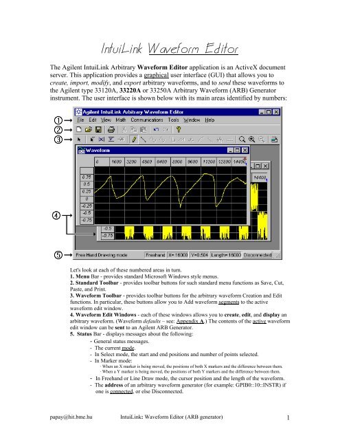
instrument. The user interface is shown below with its main areas identified by numbers: 

Let's look at each of these numbered areas in turn. 

1. Menu Bar - provides standard Microsoft Windows style menus. 

2. Standard Toolbar - provides toolbar buttons for such standard menu functions as Save, Cut, 

Paste, and Print. 

3. Waveform Toolbar - provides toolbar buttons for the arbitrary waveform Creation and Edit 

functions. In particular, these buttons allow you to Add waveform segments to the active 

waveform edit window. 

4. Waveform Edit Windows - each of these windows allows you to create, edit, and display an 

arbitrary waveform. (Waveform defaults – see: Appendix A.) The contents of the active waveform 

edit window can be sent to an Agilent ARB Generator. 

5. Status Bar - displays messages about the following: 

- General status messages. 

- The current mode. 

- In Select mode, the start and end positions and number of points selected. 

- In Marker mode: 

· When an X marker is being moved, the positions of both X markers and the difference between them. 

· When a Y marker is being moved, the positions of both Y markers and the difference between them. 

- In Freehand or Line Draw mode, the cursor position and the length of the waveform. 

- The address of an arbitrary waveform generator (for example: GPIB0::10::INSTR) if 

one is connected, or else Disconnected. 

papay@hit.bme.hu IntuiLink: Waveform Editor (ARB generator) 1

Connecting to Instrument: 

From Communications 

menu select Connection … 

• Make sure that your 

Instrument is 

physically connected 

to your computer and 

turned ON. 

• In the Connection Dialog highlight the address from the Select Address and click 

Identify Instrument. (Or double-click to perform Identify task.) The instrument 

type, name and address appear. Highlight the instrument that you wish to connect 

and click Connect. (Or double-click to Connect to it.) 

• A green icon appears to the left of instrument that is connected. 

• Once you have established a connection, click OK. Waveform Editor will 

remember the connection for any future sessions. If the instrument I/O address is 

changed, be sure to reset the connection. 

You are now ready to send waveform to the instrument. 

Configuration of Waveform Edit Window parameters: 

See – Appendix A. 


About arbitrary waveforms 

For most applications, it is not necessary to create an arbitrary waveform with a specific 

number of points since the 33220A ARB generator will repeat points (or interpolate) as 

necessary to fill waveform memory. 

For standard waveforms, and arbitrary waveforms that are defined with fewer than 16,384 

(16K) points, the function generator uses waveform memory that is 16K words deep. For 

arbitrary waveforms that are defined with more than 16K points, the function generator uses 

waveform memory that is 65,536 (64K) words deep. 

The 33220A represents amplitude values by 16,384 discrete voltage levels (or 14-bit vertical 

resolution). The specified waveform data is divided into samples such that one waveform 

cycle exactly fills waveform memory. If you create an arbitrary waveform that does not 

contain exactly 16K or 64K points, the waveform is automatically “stretched” by repeating 

points or by interpolating between existing points as needed to fill waveform memory. 

For the 33220A, you do not have to change the length of the waveform to change its 

output frequency. 

All you have to do is create a waveform of any length and then adjust the function generator’s 

output frequency. However, in order to get the best results (and minimize voltage 

quantization errors), it is recommended that you use the full range of the waveform DAC: 

from –1 to +1 relative amplitude (or 0 to 16381 [14-bit] DAC codes). 

Remember, if you create an arbitrary waveform that includes three cycles of a waveshape 

(for example), the output frequency will be three times the value displayed on the function 

0generator’s front panel. 

When creating arbitrary waveforms, the function generator will always attempt to 

replicate the finite-length time record to produce a periodic version of the data in 

waveform memory. However, as shown below, it is possible that the shape and phase of a 

signal may be such that a transient is introduced at the end point. When the waveshape is 

repeated for all time, this end-point transient will introduce leakage error in the 

frequency domain because many spectral terms are required to describe the discontinuity. 

Leakage error is caused when the waveform record does not include an integer number of 

cycles of the fundamental frequency. Power from the fundamental frequency, and its 

harmonics, is transferred to spectral components of the rectangular sampling function. Instead 

of the expected narrow spectral lines, 

leakage can cause significant 

spreading around the desired spectral 

+1 

peaks. You can reduce leakage errors 

by adjusting the window length to 

include an integer number of cycles 

(+1) 

or by including more cycles within 

-1 

the window to reduce the residual 

end-point transient size. 

Some signals are composed of discrete, non-harmonically related frequencies. Since these 

signals are non-repetitive, all frequency components cannot be harmonically related to the 

window length. You should be careful in these situations to minimize end-point 

discontinuities and spectral leakage. 


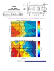
About signal imperfections 

33220A type ARB generator (14-bit, 50 MSa/s, 64K [or 16K] points) 1 

For sine waveforms, signal imperfections are easiest to describe and observe in the 

frequency domain using a spectrum analyzer. Any component of the output signal, which 

has a different frequency than the fundamental (or “carrier”) is considered to be spurious. 

The signal imperfections can be categorized as harmonic, non-harmonic, or phase noise 

and are specified in “decibels relative to the carrier level” or “dBc”. 

Harmonic Imperfections Harmonic components always appear at multiples of the 

fundamental frequency and are created by non-linearities in the waveform DAC and other 

elements of the signal path. 

Non-Harmonic Imperfections The biggest source of non-harmonic spurious components 

(called “spurs”) is the waveform DAC. Nonlinearity in the DAC leads to harmonics that are 

aliased, or “folded back”, into the passband of the function generator. These spurs are most 

significant when there is a simple fractional relationship between the signal frequency and the 

function generator’s sampling frequency (50 MHz). 

For example, at 15 MHz, the DAC produces harmonics at 30 MHz and 45 MHz. These 

harmonics, which are 20 MHz and 5 MHz from the function generator’s 50 MHz 

sampling frequency, will appear as spurs at 20 MHz and 5 MHz. 

Another source of non-harmonic spurs is the coupling of unrelated signal sources (such as the 

microprocessor clock) into the output signal. These spurs usually have a constant amplitude 

(< -75 dBm or 112 µVpp) regardless of the signal’s amplitude and are most troublesome at 

signal amplitudes below 100 mVpp. To obtain low amplitudes with minimum spurious 

content, keep the function generator’s output level relatively high and use an external 

attenuator if possible. 

Phase Noise Phase noise results from small, instantaneous changes in the output frequency 

(“jitter”). It is seen as an elevation of the apparent noise floor near the fundamental frequency 

and increases at 6 dBc / octave with the carrier frequency. The 33220A’s phase noise 

specification represents the amplitude of the noise in a 1 Hz bandwidth, 10 kHz away from a 

20-MHz carrier (-115 dBc/Hz, typical). 

Quantization Errors Finite DAC resolution (14 bits) leads to voltage quantization errors. 

Assuming the errors are uniformly distributed over a range of ±0.5 least-significant bit (LSB), 

the equivalent noise level is -86 dBc for a sine wave that uses the full DAC range (16,384 

levels). Similarly, finite-length waveform memory leads to phase quantization errors. 

Treating these errors as low-level phase modulation and assuming a uniform distribution over 

a range of ±0.5 LSB, the equivalent noise level is -76 dBc for a sine wave that is 16K samples 

long. All of the 33220A’s standard waveforms use the entire DAC range and are 16K 

samples in length. Any arbitrary waveforms that use less than the entire DAC range, or that 

are specified with fewer than 16,384 points, will exhibit proportionally higher relative 

quantization errors. (Note: arbitrary waveform length 2 to 64K points.) 

With the 33220A, you can output an arbitrary waveform to an upper frequency limit of 6 

MHz. However, note that the useful upper limit is usually less due to the function 

generator’s bandwidth limitation and aliasing. Waveform components above the function 

generator’s -3 dB bandwidth will be attenuated. 

1 Signal imperfection for 33120A type ARB generator – see Appendix B. 


About on-line help 

The Waveform Editor Help provides the following help books in the table of contents: 

· Introduction to the Waveform Editor provides a short introduction to the waveform editor 

application. 

· Using the Waveform Editor provides task-oriented how-to topics on how to use the waveform 

editor. 

· Waveform Editor Reference provides a reference topic for each waveform editor command or 

dialog box. 

Note: 

Certain standard dialog boxes such as Communication | Connection or Send; Math | 

Filter | Low Pass; Math | Waveform Math; Tools | FIR Filter etc. have a help. Click 

on this button, and then click on the area of interest in the dialog box to obtain help 

for these dialog boxes. 


Creating and editing waveforms: 

SAVE 

Cut, Copy, Paste 

HELP 

New, Open 

PRINT 

Undo, Redo 

Select 

Markers 

Freehand 

and Line 

drawing 

Standard 

waveforms 

Zoom 

in/out 

SEND 

(download) 

Inserting a segment 

You can insert standard waveform segments using the waveform toolbar icons. When you 

click the desired icon the segment is inserted (with its default parameters) in the active 

waveform edit window. 

blue 

triangle 

standard waveform segments 

(+1) 

(-1) 

To change the parameters (or waveform) of an existing segment, double-click on the segment 

and Segment Parameters dialog box appears. 

You can insert standard waveform segments using the menu (Edit | Insert Segment) and 

the Segment Parameters dialog box. 

You can continue to insert segments to an existing waveform, provided there is room 

in the edit window for the segment to be inserted. Segments are always inserted on 

the right side of the waveform. 


Drawing an Arbitrary Waveform 

Freehand mode allows you to draw any shape that you want, while Line Draw mode 

allows you to draw a series of straight lines. 

Both Freehand and Line Draw mode may be used anywhere within the window, 

except where a standard segment has been inserted. If the window already contains a 

waveform segment, the drawing will start at the right edge of that segment. 

Selecting (i.e. highlighting) waveform data 

You can select all or a portion of a waveform as described below. 

Note: Once you have selected the waveform data, you can operate on the data 

with one of the Math menu functions, or with Cut, Copy, or Paste in the Edit 

menu. 

1. To select a standard waveform segment within the waveform: 

Click on the small blue triangle above the waveform segment. 

Or, double-click anywhere within the waveform segment. 

2. To select the entire waveform: 

In the Edit menu (or after right mouse click within waveform window), click 

on Select All. 

3. To select a portion of the waveform: 

If you are not already in Select mode, click on the icon in the toolbar (or 

from the Edit menu click on Select). 

Click the left mouse button at the start of the desired portion of the waveform, 

drag, and release the mouse button when the desired area is highlighted. (You 

can drag either left-to-right or right-to-left.) 

Using Markers (click on the icon) 

Markers can be used as guides for freehand or line drawing, or to specify an area of a 

waveform to be clipped. 

In Marker mode, when you move an X marker, the X marker positions are shown in the 

status bar. When you move a Y marker, the Y marker positions are shown in the status 

bar. 

Use Pin Markers to define an area where you can perform freehand or line 

drawing over standard segments. You can draw only in the area defined within the 

pinned X and Y markers. (Note that any potential discontinuities at the ends of the 

freehand area are automatically corrected with straight lines connecting to the original 

waveform.) 

The pinned markers change color and the handles disappear. You cannot move markers 

that are pinned. 

Clipping a Waveform: The Clip math function clips the selected waveform data to 

the specified Y values. Position the markers to the desired clipping values (click and 

drag the triangular handles at the left end of the markers), select the portion of the 

waveform, then Clip the waveform (from the Math menu select Clip) to the values 

specified by the pinned Y markers. 


Zoom using a ‘magnifying glass’ 

Allows you to zoom into a specified area of the waveform edit window. Select Zoom 

to turn zoom mode on. The cursor changes to a magnifying glass. 

‘leakage 

error’ 

The zoom locator box in the Thumbnail View window outlines the portion of the 

waveform currently displayed in the waveform edit window. This box changes as you 

zoom in and out and can be moved by clicking and dragging it. 

Sample Files 

Use File | Open … or click the File Open icon to open these files. Once open, the 

waveform can be edited, inserted, or copied. 

see: Appendix C 

Importing waveform from Scope 

See: Tools | Import Waveform (Agilent 546xx Scope) 


Performing waveform Math 

The Math menu contains several math functions to be performed on waveforms. The 

first three (add, sub, and mult) combine two operands (point-by-point) while the 

remaining functions performed on a single operand. 

Note: The first waveform is the waveform or portion of a waveform that you have 

selected (i.e. highlighted) in the active waveform edit window. The second waveform is 

either a standard waveform or a waveform that has been copied to the clipboard. 

The Windowing or the Low Pass filter function always applies to the entire waveform, 

whether or not the waveform or a portion of it has been selected. 

The Extended Cosine, Raised Cosine, and Hamming windowing functions can be used to correct 

for distorted spectral information where there are discontinuities at the end point of the window, or 

when the frequency components of the waveform are not harmonically related to the window 

length. (More filter … Tools | FIR Filter.) 

By default, the Smoothing filter performs a 7-point moving average. However, you can 

change the number of points from the Properties dialog box (from the File menu, select 

Properties). 

Example: 

sin 2 x 

sin 3 x 

More Math … Tools | Equation Calculator; Tools | Pulse Maker. 


Send Arbitrary Waveform: 

Click on the icon in the waveform toolbar (or select the ‘Send Waveform …’ 

command from the Communications menu) to display the Send Arbitrary Waveform 

dialog box. 

Note: 

If you click on the icon or ‘Send Waveform …’ command when no instrument is 

connected, the Connection dialog box appears. (See Connecting to Instrument.) Once a 

connection has been established, the Send Arbitrary Waveform dialog box appears. 

The dialog box provides two tab pages. 

Manage Waveforms Tab: 

Activate or delete the waveforms currently in the instrument’s memory. 

Waveforms on the Instrument: 

Lists the available waveforms stored on the instrument. 

• To activate one of the waveforms, select its name and click on the 

Activate button. 

• To delete one of the non-permanent waveforms from the instrument, 

select its name and click on the Delete button. 

Permanent, built-in waveforms are indicated with an asterisk (*) preceding the 

name. These waveforms cannot be deleted from the instrument. Also, you cannot 

delete the currently active waveform. (To get around this, activate a different 

waveform and then select the one that you want to delete.) 


Send Waveform Tab: 

Specify parameters and then send (download) of the contents of the active 

waveform edit window to previously connected instrument. 

Waveform Parameters: 

• Frequency (kHz): The function generator repeat-frequency. 

• Amplitude (Vp-p): The peak-to-peak amplitude of the repeating waveform. 

• Offset (Vdc): The dc offset to the waveform. 

Reset Parameters: 

Click on Reset to restore the selected parameters: 

• Defaults for Waveform: The default parameters saved with the waveform in the file. 

• Current from Instrument: The current parameters retrieved from the instrument. 

Waveform Location on Instrument: 

• Volatile Memory: Save the waveform in the instrument's volatile memory. 

• Memory Name: Save the waveform in the named location on the instrument. 

Send to Instrument: 

• Waveform and Parameters: Send the waveform and its parameters. 

• Waveform Parameters Only: Send only the parameters to save time when the waveform 

has already been sent. 

Once you have specified all the parameters, click on Send to send the waveform 

to the instrument. A message is then displayed with an estimated time to complete 

the send operation. (Click OK.) 


Supported Data File Formats: 

The Agilent IntuiLink Arbitrary Waveform Editor supports several data file formats, 

which are listed below. 

Data files can be saved with the Save and Save As commands, and opened with the 

Open command from the File menu. 

1. Waveform (.WVF) File Format. This is the default format used for arbitrary 

waveform files saved using the waveform editor. 

2. Comma-Separated Values (.CSV) File Format. This format uses the comma 

as the delimiter between columns, and a carriage-return/line-feed to terminate 

each row. 

- The waveform editor reads .CSV files from Microsoft Excel and other 

applications. The waveform editor reads the last column containing data as 

the waveform data column to be compatible with Agilent BenchLink Arb 

and most other applications including Excel. 

- The waveform editor saves .CSV files in a special format, shown below in 

an Excel spreadsheet: 

Row 1 is used to store the column headers. The waveform data points are saved 

in the column A, which may be several thousand points in length. Succeeding 

columns are used to store the waveform parameters. In our example, columns 

B through F store the name, frequency, amplitude, offset, and number of points 

in the waveform. 

Note: 

The .CSV file format supports only the US English number format, with 

periods used as decimal points. This is because the comma is used as the 

delimiter. (See Appendix D.) 

3. Text (.TXT) File Format. This format puts all of the data points in a single 

column, with a carriage-return/line-feed after each value. 

If you read the file into Excel, the data points will be in column A, and that 

column may be several thousand points in length. This format can be used 

with localized number formats (for example, using the comma as the decimal 

point). 


4. Text (.PRN) File Format. This format puts all of the data points in a single 

row, using the space as the delimiter between data points. 

If you read the file into Excel, the data points will be in row number 1, and 

that row may be several thousand points in width. This format can be used 

with localized number formats (for example, using the comma as the decimal 

point). 

5. Picture (.BMP) File Format (Save Only). You can save a raster 

representation of your waveform in a Windows Bitmap (.BMP) file. 

This makes it convenient to include a picture of your waveform in Microsoft 

Word or other applications. 

However, this picture no longer consists of waveform data. You cannot open a 

.BMP file in the waveform editor, and you will need to save your waveform 

data in one of the other supported formats. 

(Note: There is also a waveform setup file format (.WFG), which is used to save the 

current instrument setup for type 33250A ARB generator: File | Save, Load ...) 

Printing waveforms: 

Click on the icon to output a printout using the current configuration. 

From the File menu select either Print or Print Preview to display the Print dialog box. 

This dialog box provides two tabs: the Preview tab shows what your printout will look 

like with the current layout; go to the Page Layout tab page to change the layout. 


Tools: 

Tools | Import Waveform (Agilent 54622A Scope) 

From the Tools menu, select Import Waveform (Agilent 546xx Scope) to display 

dialog box. The dialog box provides two tab pages. From the Waveform tab page 

you can specify parameters for importing a waveform. From the Connect to 

Oscilloscope tab page you can establish a connection to your oscilloscope. 

Waveform Tab: 

· Currently Connected Oscilloscope: Shows the address of the currently connected 

oscilloscope. 

If no scope is connected, go to the Connect to Oscilloscope tab. 

· Channel: Specify the oscilloscope channel to import. 

· Number of Points (Agilent 546xx only): Specify the number of points to import. 

Connect to Oscilloscope Tab: 

The Oscilloscope Address is shown. To connect an oscilloscope, click on the Connect to 

Oscilloscope button. The Connection Dialog box appears. 


Tools | Equation Calculator 

Creates noise waveforms (see: next page) or waveform from mathematical 

expressions (see: Appendix E). Use the View page to verify that you’ve built the 

waveform you want. 


Examples: “colors of noise” 

Many test of electronic equipment and components use white noise, pink 

noise or Brown noise. The figures show the four of noise plotted and 

Fourier transformed with Equation Calculator (4000 points) 

uniform, white 

normal (Gaussian), white 

pink, 1/f (-10dB/decade) 

Brown, 1/f 2 (-20dB/decade) 

W. Haussmann: Create noise and signals with software 

Test & Measurement World, Sept. 2002. WEB site: http://www.e-insite.net/tmworld/ 


Tools | Pulse Maker 

Creates pulse waveforms with variable rise/fall time. The shapes for the rise/fall 

times can be Linear, Exponential, Half-Cosine or Gaussian. 

Intended for use with slow (> 100 nsec) rise/fall times. 

1 mHz to 5 MHz 

33220A: max 64K points 

(33120A: max 16K points ) 

Note: after saving in a file, you can export (download) the pulse waveform with ‘Reset parameters’ in 

‘Send waveform’ tab to ‘Default for Waveform’. 


Tools | FIR Filter 

FIR filter Tool requires data in the active waveform edit window! When you click 

OK in any tab, the tool will apply the selected (Kaiser or moving-average) filter to the 

data and then plot the filtered waveform. 

Note: number of filter term (N) increases 

as you shorten ft, which creates a sharper 

transition. 

But N increases only as the log of the 

ripple increase. 

W. Haussmann: Filter your data in software 

Test & Measurement World, April 2002. WEB site: http://www.e-insite.net/tmworld/ 


Appendix: 

(A) Parameters for all Waveform editor Windows: File | Properties … 

33120A type ARB generator: 16K points and 12 bits resolution 

33220A type ARB generator: 64K (or 16K) points and 14 bits resolution 

33250A type ARB generator: 64K points and 12 bits resolution 


(B) About signal imperfections - 33120A type ARB generator (12-bit, 40 Msa/s, 16K) 

Most signal imperfections are easiest to observe in the frequency domain using a 

spectrum analyzer. Sampling theory predicts the location and size of spurious signals 

resulting from the sampling processes used by DDS generators. 

In fact, since DDS generators use a fixed sampling rate (40 MHz for the 33120A), spurious 

signals can be removed with a fixed frequency “anti-alias” filter. 

A 17 MHz, ninth-order elliptical filter providing a sharp cut-off (in excess of 60 dB attenuation for 

signals greater than 19 MHz) is used for sine wave outputs. A 10 MHz, seventh-order Bessel filter 

is used for non-sine wave outputs. The Bessel filter provides slower amplitude roll-off for antialias 

filtering, but maintains linear phase response to minimize shape distortion for complex 

waveshapes. The 33120A automatically selects the appropriate filter when the output function is 

selected. 

All digital-to-analog converters (DACs), including those used in DDS generators, 

produce spurious signals resulting from non-ideal performance. These spurious 

signals are harmonically related to the desired output signal. At lower frequencies, the 

33120A’s 12-bit waveform DAC produces spurious signals near the -74 dBc level 

(decibels below the carrier or output signal). The 33120A uses the complete vertical 

resolution (N=1) of the DAC for all internal waveshapes, thus minimizing amplitude 

quantization error. 

At higher output frequencies, additional DAC errors produce non-harmonic spurious outputs. 

These are signals “folded back” or aliased to a frequency within the signal bandwidth. A “perfect” 

DAC will also produce a wideband noise floor due to amplitude quantization. The noise floor for a 

12-bit DAC will be near the -74 dBc level; this corresponds to a noise density of -147 dBc/Hz for 

sine wave outputs 2 from the 33120A. 

Another type of waveform error visible in the frequency domain is phase truncation 

error. This error results from time quantization of the output waveform. Whenever a 

waveshape is described by a finite number of horizontal points (length), it has been 

sampled in time (or quantized) causing a phase truncation error. Spurious signals 

caused by phase truncation introduce jitter into the output waveform. This may be 

regarded as time (and phase) displacement of output zero crossings. 

Phase truncation causes phase modulation of the output signal which results in spurious harmonics 

(see the equation below). For lower output frequencies, the phase accumulator periodically does 

not advance RAM addresses, causing the DAC to deliver the same voltage as recorded on the 

previous clock cycle. Therefore, the phase “slips” back by 360 0 / points before continuing to move 

forward again. When RAM address increments are the same on each cycle of the output, phase 

truncation error (and jitter) are essentially zero. All standard waveshapes in the 33120A are 

generated with at least 16,000 waveform points which results in spurious signals below the wideband 

noise floor of the DAC. 

2 The noise power is normalized to a 1 Hz bandwidth by simply subtracting 

6 

10 ⋅ log( f / 2) = 10 ⋅ log(40 ⋅10 

/ 2) = 73 from the SNR value. 

sample 


(C) Sample files: 

File name Description Size (N o of points) 

Dtmf_0.csv 

Dtmf_9.csv 

Telephone Dual Tone Multi-Frequency 

(DTMF) Signal – Key 0 (really: Key * ) 

Send : 10 Hz 

Telephone Dual Tone Multi-Frequency 

(DTMF) Signal – Key 9 

Send: 10 Hz 

8K 

8K 

Full_rec.csv Full wave rectified sine wave 8K 

Gaussian pulse created in Mathcad 

Gausian.csv and imported 

8K 

Half_rec.csv Half-wave rectified sine wave 8K 

74HC family digital signal, captured 

Hc_Gate.csv and imported from HP BenchLink/Scope 4K 

NoiseSine.csv Sine wave with high frequency noise added 8K 

nonlin_1.csv 

Sine wave with third harmonic distortion 

(Fourier synthesis) 

8K 

Pk_spike.csv Sine wave with spike added to each peak 8K 

Psk.csv Phase Shift Keying modulated signal 8K 

Pulse_10.csv 10 level sine wave approximation 8K 

Square wave with ringing 

(Fourier synthesis) 

Ring.csv 

4K 

Scr.csv Quarter cycle SCR signal 8K 

Serial.csv 11-bit frame of serial data 4K 

0.1% duty cycle square wave signal 

Sm_duty.csv 

Send: 100 Hz 

4K 

Stair.csv 10 step staircase ramp signal 8K 

Trapazd.csv Trapeziodal pulse ** 4K 

TwoTone.csv 

8K 

Two tone signal for intermodulation test 

Send: 70 Hz 

** Example: if you cut the last 1K points from a ‘Trapazd’ segment, you get a 

50% duty cycle trapezoidal pulse series with the following spectrum: 

r 

1 

3 

[dB] 

TRAP( pr , ) 

0 

20 

40 

60 

spektrum 

80 

1 51 101 

Send (download): 1 kHz 

Oscilloscope screen image 

with IntuiLink Toolbar 

(for Word): 

k 

p 

k 

1 

3 

5 

7 

9 

11 

13 

15 

17 

TRAP( k, 

r) 

0 

13.1 

28 

33.8 

32.1 

41.7 

44.6 

41 

49.2 

[dB] 


(D) Exporting waveform to Excel: 

If you want to export waveform data from the waveform editor to Microsoft 

Excel, you can save the data as a .CSV file. Follow these steps: 

1. Create and edit the waveform to be saved. 

2. From the File menu, select Save As. The Save Waveform As dialog box 

appears: 

a. Enter a name in the File Name field. 

b. For Save as Type, select CSV (comma delimited) (*.CSV). 

c. Click on Save to save the file. The .CSV extension is appended 

to your file name automatically. 

3. The file is now saved as a .CSV file, and can be read into Microsoft Excel. 

Note: 

The .CSV file format uses the comma as the delimiter. Therefore, the European 

localized number format cannot be used, with commas as the decimal point. 

However, the waveform editor also can export files in the .TXT file format, which 

does support localized number formats (see Supported Data File Formats). 


(E) Waveform: Equation ( Amplitude: -1 to +1, Total number of points: 4000 ) 

Operator menu: +, -, *, /, ^ (raise to the power), ( , ) – parentheses, pi (3.1416), 

t (time 0-1), w (2*pi*t), var (variable), 1 = .1E1 – numerals 

Function menu: 

Abs(), ArcTan(), Cos(), Exp(), Fact(), Ln() 

Noise(1) uniform, Noise(10) normal 

Point(), Sin(), Sqrt(), Step(),Tan() 

Sample menu: 

Time reversed step 

(Step Down), 

alternate: –Step(t-.5) 

Step, rise: Step(t-.5) 

Step, fall: Step(.5-t) 

Step function creates a unit step at the location 

specified by the argument (or function) 

Step at point 1000: Step(t-Point(1000)) 

Pulse, alternate: Step(var)-Step(var-0.2) 

Pulse 20% duty cycle: Step(var)*Step(0.2-var) var = t-.5 

Pulse negative: Step(var)+step(-(var+.2)) 

var = .5-t 

Step function accepts other functions, f(t), as an argument: 

Step(f(t) > 0) = 1, and Step(f(t) < 0) = 0 

Pulse train: Step(Sin(5*w)) , pulse frequency: 5 

Sine, one cycle: Sin(w) or Sine, alternate: Sin(2*pi*t) 

Sine, 2 cycles: Sin(2*w) 

Sine, 45deg offset: Sin(w-pi/4) 


Sine, burst: Step(var)*Step(1/10-var)*Sin(10*2*pi*var) 

var = t-.4 

Sine, burst 3 cycles: Step(var)*Step(3/10-var)*Sin(10*2*pi*var) 

var = t-.4 

Noise(5): the argument “5” tells Equation Calculator to take the average 

of five random values and use the result for the value of the noise( ) function. 

Note: averaging a random set of numbers produces a Gaussian distribution, 

which produces a more realistic noise signal then pure white noise. 

Sine with noise burst: Sin(w)+Step(.01+var)*Step(.01-var)*Noise(5) 

var = t-.25 

Sine(x)/x: Sin(5*w)/w 

Impulse: Sin(25*var)/var 

var = 2*pi*(t-.5) 

Impulse, windowed: (1-cos(w))*Sin(25*var)/var var = 2*pi*(t-.5) 

Ramp: t 

Ramp, negative: .5-t 

Ramp, partial: Step(var)*Step(.3-var)*var 

var = t-.2 


Exponential, decay: Exp(-5*t) 

Exp, rise: 1- Exp(-5*t) 

Damped Sine: Exp(-5*t)*Sin(10*w) 

Gaussian pulse: exp(-0.5*((t-Tm)/To)^2) 

Tm – time location of center or “mean” of Gaussian pusle 

To – half width of Gaussian point corresponds to standard deviation 

Gaussian: Exp(-.5*((t-.5)/.1)^2) 

Ringing square wave: 

Step(-var)*(.2*Exp(-15*t)*Cos(50*w)+1)-Step(var)*(.2*Exp(-15*(var))*(Cos(50*2*PI*(var)))+1) 

var = t-.5 

Modulation, AM: Sin(20*w)*(1+0.75*Cos(2*w)) 

Modulation, frequ.: Sin(20*w+10/2*Cos(2*w)) 

Modulation, phase: Sin(20*w+pi*Sin(2*w)) 

Modulation, pulse width: 

step(sin(20*w+var*cos(1*w)))*step(sin(20*w+var*sin(1*w))) 

var = pi/2 

Rectified, full wave: Abs(Sin(3*w)) 


Rectified, half wave: .5*(Abs(var)-var) 

var = sin(3*w) 

Window, extended cosine bell: 2-(1+cos(5*w))*(step(.1-t)+step(t-.9)) 

Window, half cycle sine: sin(.5*w) 

Window, Triangle: .5+var*Step(-var)-var*step(var) var = t-.5 

Window, Hanning: 1-cos(w) 

Window, half cycle sine^3: sin(.5*w)^3 

Window, Hamming: 0.08+0.46*(1-cos(w)) 

Window, Cosine^4: (0.5*(1-cos(w)))^4 

Window, Parzen: 

Step(var)*Step(.5-var)*(1-6*(2*t-1)^2+6*abs(2*t-1)^3)+2*(1-abs(2*t-1))^3*(step(-varpoint(1))+ 

step(var-.5-point(1))) 

var = t-.25 


Examples: 

Lorentz pulse: 1/(1+((t-Tm)/To)^2) 

Tm – time location of center 

To – half width @ 50% amplitude 

Lorentz pulse: 1/(1+((t-0.5)/0.1)^2) 

Sine^3: Sin(w)^3 

PAM (pulse amplitude modulation): t*step(sin(7*w)) 

Sine amplitude sweep: t*sin(7*w) 

LIN sweep: sin(2*pi*Fs*t+pi*(Fe-Fs)/Ts*t^2)) 

Fs – start frequency, Fe – stop (end) frequency, Ts – sweep duration 

Linear frequency sweep: sin(10*w+pi*(20-10)/0.5*t^2) 

LOG sweep: sin(2*pi*(Fs/K)*(exp(K*t)-1)), K= ln(Fe/Fs)/Ts 

Fs – start frequency, Fe – stop (end) frequency, Ts – sweep duration 

Logarithmic frequency sweep: 

sin(2*pi*(10/var)*(exp(var*t)-1)) 

var = ln(20/10)/0.5 

Multi-tone: cos(w)+cos(2*w)+cos(3*w) 

Test signal (bandwidth limited square wave): 

sin(w)+0.24*sin(3*w)+0.07*sin(5*w)+0.0125*sin(7*w) 


Combined sine and straight line: sin(1E1*w)-2*t 

Fourier transform: 

Modulation: sin(w)*cos(3E1*w) 


100 cycles of sine Amplitude Modulated with 10 cycles of sine with a modulation 

depth of 20% (note: upper and lower sidebands are defined separately and added 

to the carrier): sin(1E2*w)+.2*cos(1.1E2*w)-.2*cos(.9E2*w) 


FM broadcast stereo composite signal: left channel, sine, 1 kHz 

0.5*sin(w)+0.1*sin(19*w)+0.25*sin(37*w+pi/2)+0.25*sin(39*w-pi/2) 

20% second harmonic distortion: sin(w)+.2*sin(2*w) 

Disturbance on an AC waveform (note: the disturbance is decayed 

400Hz sine on a 50Hz signal): 1.2*exp(-t/.13)*sin(400/50*w)+sin(w) 

Chopped sinewave: sin(w)*step(sin(10*w)) 


This article appeared on the Test & Measurement World web site at www.tmworld.com. 

Create noise and signals with software 

Werner Haussmann, Agilent Technologies, Loveland, CO -- 9/1/2002 

Test & Measurement World 

Arbitrary waveform generators (AWGs) and other instruments with programmable analog outputs 

often let you use equations to create waveform points. Math functions in equations let you create 

"perfect" waveforms, without disturbances or noise in the signal. Often, though, you need to 

produce noisy waveforms to test a product's immunity to disturbances, or you need to produce 

noise signals to test your product's frequency response. 

Recently, I needed to generate numerous waveforms, both clean and noisy. I also needed to 

create noise signals. I created an ActiveX software component that lets me calculate waveforms 

with equations. It also lets you create white noise, pink noise, and Brown noise. "Types of noise" 

(below) provides descriptions and sample plots of each noise type. 

The software component, called Equation Calculator, displays 

the waveform in the time domain or in the frequency domain. 

Equation Calculator works with Visual Basic (VB) version 6 and 

.Net, and I've made it available to you at no cost. (See 

"Download instructions" for a link to the download page.) 

Manual and automatic 

The Equation Calculator has both a graphical user interface 

(GUI) and an applications programming interface (API), so you 

can operate it manually or as part of an application program. 

To open Equation Calculator's GUI, you need some code 

because Equation Calculator is an ActiveX software 

component; it's not an ActiveX control that you can use by 

dropping it into a VB form. 

Use the GUI to build and view your waveforms, then use the 

API to apply your waveforms to an automated test. I won't 

discuss equations for creating waveforms in this article. If you 

need some examples, see "Equations shape AWG waveforms" 

in the May 2001 issue of Test & Measurement World (Ref. 1). 

Download instructions 

To get the Equation Calculator, 

go to Agilent | 

33120A/33220A/33250A 

Function/Arbitrary Waveform 

Generator Equation/Noise 

Add-in. In the Software section, 

click on "33120/250A Equation 

Calculator Add-in." There, you 

can download the Equation 

Calculator ActiveX component. 

You need Visual Basic 6.0 

installed on your computer for 

the ActiveX component to 

work. 

If you have an Agilent 

33120A/250A waveform 

generator, then you can use 

Equation Calculator as an addin 

for the Agilent Waveform 

Editor application. Once 

installed, you can access the 

Equation Calculator's dialogs 

from the Tools menu.

Figure 1 shows Equation Calculator's GUI, 

which uses four tabs that take you to 

property pages. To use Equation 

Calculator, start with the Selection page. 

Here, you'll find several radio buttons that 

let you choose to either build your own 

waveform from an equation or select a 

noise signal to apply to your tests. 

Regardless which option you choose, you 

must also select the number of points in 

your waveform and the range of amplitudes 

(0 to 1, –1 to +1, or –1 to 0). 

Using the GUI, you create equations by 

selecting samples, functions, and operators 

from three menus (Figure 2). The Sample 

menu provides a selection of waveforms 

such as a sine wave burst, sine wave with 

noise, damped sine wave, amplitudemodulated 

carrier, frequency-modulated 

carrier, and square wave with ringing. The 

Function menu includes trigonometric 

functions, white noise, a step function, and 

a square root. You can use the samples, 

functions, and operators to create complex 

waveforms. An equation field lets you see 

and edit the equation. The Variable field 

displays an independent variable, usually 

time, associated with the waveform 

equation. 

The Equation field in Figure 2 shows a 

function called noise(5) that lets you add 

white noise to any equation. The argument "5" tells Equation Calculator to take the average of 

five random values and use the result for the value of the noise() function. Averaging a random 

set of numbers produces a Gaussian distribution, which produces a more realistic noise signal 

than pure white noise. The equation in Figure 2 multiplies the product of two step functions by the 

average of five random values. It then adds that result to a sine wave to produce the noise spike 

in the waveform in Figure 1. 

After you enter an equation or select a noise signal, use the View tab to see your waveform. If 

you right-click on the waveform plot, you can either copy the plot and data to the clipboard or you 

can select "Fourier Transform" to view the waveform in the frequency domain. To use or store the 

waveform's data points, paste the data to Excel and then to a file, or use the component's API in 

VB. 

Activate the ActiveX 

Figure 1. Use a free ActiveX component to 

generate waveforms such as this sine wave with 

noise. 

Figure 2. Menus let you build equations that 

represent waveforms. 

When you download and install the Equation Calculator component, you must first reference it to 

your VB project and write some code that activates it. To reference the component, use the 

Project menu, and select References. Check the box Agilent Equation Calculator Add-in and 

select OK. To activate Equation Calculator, you need a VB program that contains code such as 

2

that in Listing 1. I suggest that you create a VB project, add a command button, and place the 

code from Listing 1 into the button's code area. Run the project. Click on the button to activate 

Equation Calculator's GUI. 

Once you activate Equation Calculator, try building a few waveforms to get a feel for how it works. 

Use the View page to verify that you've built the waveform you want. Once you complete your 

equation, copy it so you can paste it into your VB code. 

Listing 2 shows how to use Equation Calculator, through its API, to create a waveform with an 

equation and place the data points in a variable. This code will create the data points for a 1000- 

point sine wave and store the points in the variable "data." In the code example, w represents 

radians, or 2πt, where t ranges from 0 to 1 in increments of 0.001. 

Note that the method EquationWaveform has three arguments. The first argument contains the 

equation. The second argument contains the number of points in the waveform. The third 

argument, breakpoint, identifies the character position of an equation-string error. For example, if 

you typed "Sun" instead of "Sin," the argument would return the position of the syntax error. 

That's useful for debugging your code. 

Equation Calculator also lets you create noise signals through its API. In Listing 3, the object equ 

contains a property called NoiseWaveform that uses two arguments. The first argument selects 

the type of noise that you want to generate, and the second sets the number of points in the 

signal. 

Table 1 lists the types of noise and their programming codes. 

The example in Listing 3 shows the code for creating a 1000-point signal that simulates white 

noise. 

Using the code examples in Listings 2 and 3, you can create a waveform and store its points in 

an array. You then can use VB to save the array to a text file or import the data into an AWG or 

other programmable analog output instrument. 

Table 1. Programming codes for noise waveforms 

Programming Code | Type of Noise: 

1 White noise with uniform distribution 

2 White noise with Gaussian distribution 

3 Pink noise 

4 Random walk 

5 Brown noise 

Author Information 

Werner Haussmann is a technical marketing manager at Agilent Technologies in Loveland, CO. He received a 

BSEE from Fairleigh Dickinson University. E-mail: werner_haussmann@agilent.com. 

Reference 

Rowe, Martin "Equations shape AWG waveforms," Test & Measurement World, May 2001. p. 59. 

www.tmworld.com/archives . 

3

Types of noise 

Many tests of electronic equipment and 

components use white noise, pink noise, 

or Brown noise. The figure shows the 

four types of noise plotted with Equation 

Calculator. 

With white noise, any amplitude is as 

likely to occur at any point as any other 

amplitude. The power spectrum of white 

noise is, therefore, independent of 

frequency (it has a flat frequency 

response). You easily can create white 

noise in software by using a randomnumber 

generator. Software random- 

Gaussian white noise, brown noise and pink noise. 

Clockwise from upper left, random white noise, 

number generators will produce random 

numbers between 0 and 1, which you often need to shift to between –0.5 and +0.5 so the 

amplitude of the noise centers at about zero. 

Unfortunately, white noise doesn't necessarily represent any naturally occurring phenomenon. 

More often, you want a Gaussian distribution of power so most of the points have a value near 

zero. Every now and then you want a point with a value of ±0.5, which a Gaussian distribution 

will give you. White noise with a Gaussian distribution is also called "normal white noise." 

Pink noise, also known as 1/f noise, is used in audio testing. It has an even power distribution 

when you view frequency on a logarithmic scale (Ref. 1). Pink noise has the same power in the 

octave 200 Hz to 400 Hz as it does in the octave 2000 Hz to 4000 Hz, which makes it sound 

natural to our ears. It's frequency power spectra rolls off at 10 dB per decade, or approximately 

3 dB per octave. 

With brown noise, the integral of white noise, each point in the waveform depends on the value 

of the previous point. Each value moves slightly from its previous position, up or down, in a 

random fashion, or "random walk." You create brown noise by adding a random number to the 

previous value. Brown noise has a frequency spectrum of 1/f 2 and has a power density roll-off 

at 20 dB per decade (6 dB/octave). The name "brown noise" comes from the Scottish botanist 

Brown, as in Brownian motion, not the color brown (Ref 2). 

References 

1. "DSP generation of Pink (1/f) Noise," www.firstpr.com.au/dsp/pink-noise 

2. Schroeder, Manfred, Fractals, Chaos, Power Laws, W.H. Freeman and Co., New York, NY, 

1991. 

4

Listing 1 

Dim TempData As Variant 

Dim data() As Double 

Dim dummy As Double 

Dim equ As agtEquation.CWaveForm 

Set equ = New agtEquation.CWaveForm 

equ.GetWaveform TempData, dummy 

If equ.WaveFormResult = vbOK Then 

data = TempData 

End If 

Listing 2 

Dim breakpoint As Long 

Dim data As Variant 

Dim m_data() As Double 

Dim equ As agtEquation.CwaveForm 


data = equ.EquationWaveform("Sin(w)", 1000, breakpoint) 

If equ.WaveFormResult vbCancel Then 

m_data = data 

End If 

Listing 3 


Dim m_data() As Double 

Dim equ As agtEquation.CWaveForm 


data = equ.NoiseWaveform(1, 1000) 

If equ.WaveFormResult vbCancel Then 

m_data = data 

End If 

Reed Business Information, a division of Reed Elsevier Inc. All Rights Reserved. 

5

This article appeared on the Test & Measurement World web site at www.tmworld.com. 

Filter your data in software 

Werner Haussmann, Agilent Technologies, Loveland, CO -- 4/1/2002 

Test & Measurement World 

When you capture waveform data, you often want to process the data to extract information about 

the signal or to extract a particular wave shape. Filters—analog or digital—often provide the 

signal processing you need. Analog filters process signals before you digitize them. Digital filters, 

which apply software algorithms to digitized waveforms, can work in digital signal processors for 

"real-time" filtering. You can also use digital filters that run on a PC to process data you've 

already captured. 

Filters act on specific frequency components. With a filter, you can isolate wanted frequencies 

(pass band) from unwanted frequencies (stop band). Digital filters isolate frequencies by applying 

mathematical formulas called transfer functions to data points. The characteristics of a transfer 

function define a filter's frequency response. 

While working on a recent project, I needed to capture a signal, remove unwanted high-frequency 

noise, and store the "clean" signal in a file. Then, I needed to load the clean signal data into a 

waveform generator. 

To filter the data, I developed a digital filter 

in Visual Basic 6.0 that runs under Windows 

98 or 2000 (I haven't tested it under XP). 

The filter works on data I've already 

captured, plots raw and filtered data, and 

displays a filter's frequency response. 

Figure 1 shows how well the filter removes 

noise from a sine wave. 

You can download a free copy of the filter, 

which resides in an ActiveX control, and 

use it in your own programs or in an 

application program I wrote. ("Using the 

filter," below.) You also can download the 

complete source code for the filter control 

and the accompanying application. 

Figure 1. A digital filter removes unwanted 

frequency components such as noise from the 

upper trace to produce the filtered lower trace.

How digital filters work 

The simplest form of digital filter uses a moving average. A 

moving-average algorithm simply takes a number of 

surrounding points and averages their amplitudes to create a 

new point. Moving averages find use in temperaturemonitoring 

applications because they reduce the impact of 

electrical noise that can couple into signal wires. 

Figure 2 introduces notation you can use to develop a moving 

average into a digital filter. Each box in the left column 

represents a point in the data array. The boxes in the right 

column represent a seven-point moving average. Each of the 

seven boxes becomes a "term" of the filter, in which each 

term has a coefficient. For the moving average, each 

coefficient equals 1/7 (you could also make each coefficient 

equal 1, and then divide the sum by 7), which gives each term 

equal weight. When you apply equally weighted coefficients, 

you apply what is commonly called a "rectangular window" to 

the data. 

Figure 3 shows an example of how a moving average 

changes a signal. A 25-point data set contains a pulse that is 

10 points wide (green trace). The blue trace shows the result 

of applying a seven-point moving average to the pulse. The 

waveform transitions occur more smoothly in the blue trace 

than in the green trace. 

Figure 2. A moving average 

algorithm takes samples, sums 

them, and divides them by the 

number of samples. This 

example shows a seven-point 

moving average. 

Figure 3. The waveforms show a 10-point pulse (green trace) after applying a 

seven-point moving-average filter (blue trace). Adjusting the relative weights of 

the filter’s coefficients removes sharp corners (red trace). 

Note the change in the value of the moving average starting at point 3 of the blue trace. While 

that change is smoother than at point 6 of the green trace, it's still abrupt. By changing the 

relative weight of the coefficients in the moving average, you can further smooth the transition 

into the filter (red trace). For example, you can reduce the relative weight of coefficient C3 to half 

that of the other coefficients. Doing so produces a weighted moving average. But the sum of the 

coefficients must equal 1, so you can't simply set the two occurrences of C3 to 1/14 and leave the 

others at 1/7. To retain the sum, you must set coefficients C0, C1, and C2 (five coefficients 

because C1 and C2 appear twice) equal to 1/6 and set C3 equal to 1/12. The sum of the 

coefficients is (5 x 1/6) + (2 x 1/12) = 1. Tapering the windows gives less emphasis to points 

farther from point N in Figure 2. 

2

Figure 3 shows the effects of moving averages in the 

time domain. Moving averages also affect signals in 

the frequency domain. Figure 4 contrasts the 

frequency response of the equally weighted moving 

average, or rectangular window (blue trace), against 

the weighted moving average, or tapered window 

(red trace). Tapering the relative weights of the 

coefficients reduces the bumps in the stop band, 

which increases the filter's attenuation. But the better 

attenuation comes at a price—the transition 

bandwidth between the pass band and the stop band 

widens. 

By modifying the coefficients, you can improve a 

filter's response. For example, increasing the number 

of points in a filter window will improve ripple (provide 

greater attenuation) without a loss in transition 

bandwidth. 

Figure 4. In a seven-point moving 

average, applying equal weights to each 

coefficient produces the frequency 

response in the blue trace, but changing 

the weights can reduce ripple at the 

expense of a wider pass band (red trace). 

An ideal filter, if one existed, would multiply all 

frequencies in its pass band by 1 and all frequencies in its stop band by 0 with zero bandwidth 

between the two regions. This theoretical filter's transfer function requires an infinite number of 

terms. Unfortunately, calculating the coefficients for an ideal filter takes forever. Therefore, you 

must limit the number of coefficients in a filter's transfer function to make it practical to use. In my 

digital filter, I employ a Kaiser filter to process the data because it's easy to program. (You don't 

need to know how to calculate the coefficients in a Kaiser filter to use my program, because my 

code does that for you, but you can learn how the calculations work by reading "How to 

calculate Kaiser coefficients," below.) 

To use a Kaiser filter, you simply specify filter type 

(high pass or low pass), the filter's cutoff frequency 

(f c ), transition bandwidth (f t ), and ripple (Figure 5). 

You must express f t as a fraction of your digitizer's 

sampling frequency. The value of f t must always be 

less than half the sampling frequency. Frequencies 

above 0.5 times the sampling frequency will alias, 

and the filter won't produce useful results. Ripple 

represents a fraction of the pass band amplitude that 

you can tolerate in the stop band and in the pass 

band itself. For example, 1% = 0.01, and 

Figure 5. To use a Kaiser filter, you must 

specify the cutoff frequency, transition 

frequency, and percent of ripple. 

Before you download the filter, you should understand its limitations. In theory, the filter should 

attenuate frequencies in the stop band by as much as 100 dB. In practice, though, you'll get 

attenuation between 40 dB and 50 dB, which should be sufficient for most applications. 

Attenuation is limited because I used 64-bit (15-digit) precision for the variables that represent the 

coefficients. At that precision, some of the coefficients are so small that their values consume less 

than the weight of one digit. Visual Basic 6.0 lets you double the precision, but doing so doubles 

the time the program takes to calculate the coefficients. For my application, 40 dB of attenuation 

3

was sufficient. If your application requires greater precision, you can modify the filter's source 

code. 

In my project, I filtered a captured waveform and loaded the filtered signal into an arbitrary 

waveform generator. If you use an arbitrary waveform generator to reproduce the filtered 

waveform, then calculating coefficients with 64-bit precision is more than sufficient. Most 

waveform generators resolve signals to just 12 bits or 16 bits, so a better-filtered data set won't 

produce a cleaner waveform. 

Another limitation of using the filter comes from the time required to calculate the coefficients, 

which depends on the number of samples in your waveform, the width of f t , and the amount of 

ripple in your stop band. If your waveform has just 1000 points, even a slow computer will quickly 

calculate the coefficients. If your waveform contains tens of thousands of points, though, you may 

have to wait a while. For calculations that take longer than 10 s, the application program will 

estimate the calculation time so you'll know the computer didn't crash. 

Using the filter 

Instructions for downloading the software 

You can download a stand-alone application that lets 

you use the FIR filter, or you can download the filter's 

source code and use it in your own application. To 

download either, go to www.agilent.com/find/tmwarticle. 

Under "Software" click on "Test and Measurement World 

FIR Article, April 2002." You will find some instructions, 

the application, and source code. 

You can download the filter in three different forms. The easiest to use is the stand-alone 

application, which you can begin using right away. You also can download the filter compiled into 

an ActiveX control that you can call from your own application program. Finally, you can 

download the Visual Basic 6.0 source code for the ActiveX control, which will let you study the 

filter's details and modify its operation. 

If you choose the first option, you can use the filter without writing any code. The program lets 

you load a data file, filter the data, and save the filtered data to a file. You can then reproduce the 

filtered waveform with an arbitrary waveform generator. I'll use the example that I've provided in 

the download to demonstrate how the filter works. 

To begin, I saved the data from a waveform into an ASCII, tab-delimited file. The filter assumes a 

repetitive waveform where the first point is a continuation of the last point in the data. 

4

Figure 6 shows my filter's display screen, 

from which you can select a filter and enter 

its parameters. The "Filter Type" tab lets you 

select from low-pass, high-pass, or movingaverage 

filters. For the frequency scale in 

most data-acquisition applications, you 

should select "Show frequency as a fraction 

of sample frequency." If you select "Show 

frequency as a multiple of window 

frequency," you'll see a scale from 0 to one 

half the number of points in the waveform 

that you want to filter. Remember, to meet 

the Nyquist criterion, the "window" that you 

apply to your waveform must have fewer 

than half of the waveform's number of points 

(Ref. 1). 

Next, use the Parameters tab (Figure 7) to 

select the cutoff frequency, transition 

bandwidth, and ripple. In the "Frequency 

Response" tab (Figure 8), the calculated 

frequency response shows 100 dB of 

attenuation, but as I explained, you won't get 

that much. When you click OK in any tab, the 

application will apply the filter to the data and 

then plot the filtered waveform. You can save 

the filtered waveform in a text file. 

Figure 6. A digital-filter application program lets 

you select filter type, frequency scale, and 

destination. 

If you choose to download the ActiveX 

control, you can use it to filter data in your 

own program. Listing 1 shows an 

example in Visual Basic. In the sample code, 

the variable data (an array of doubleprecision 

variables contained in a variant) 

represents the waveform that you want to 

filter. The ActiveX control uses the function 

GetWaveForm to process the data and then 

return the filtered waveform into the variable 

data. You can use the waveform in your 

application or you can store it to a file. For a 

more detailed example of how to use the 

control, download the application program, 

which also comes with Visual Basic source 

code. T&MW 

Figure 7. Enter a fraction of your sampling 

frequency for values of cutoff frequency (fc/fs), 

transition frequency (ft/fs), and percent ripple. 

Listing 1 


Dim dummy As Double 

Dim fir As agtFirFilter.CWaveForm 

Dim result As Long 

Set fir = New agtFirFilter.CWaveForm 

With fir 

.getWaveform data, dummy 

result = .WaveFormResult 

End With 

Figure 8. The filter software calculates the number 

of terms needed to meet your needs and then 

plots the filter’s frequency response. 

5

References 

1. Moffitt, Paul, "Proper sampling ensures good data ," Test & Measurement World, July 

2001. p. 115. 

Author Information 

Werner Haussmann is a technical marketing manager at Agilent Technologies in Loveland, CO. 

He received a BSEE from Fairleigh Dickinson University 

How to calculate Kaiser coefficients 

In 1977, J.F. Kaiser and W.A. Reed published a paper (Ref. a) that described a method of 

calculating a filter's coefficients (c(k)) given values for the filter's cutoff frequency (f c ), transition 

bandwidth (f t ), and ripple (Ref. b). Their method uses the following five equations: 

Low-pass filter 

High-pass filter 

where 

k ranges from 1 to N 

N represents the number of terms in the filter's transfer function 

w(k) represents a Kaiser-Bessel window; the window alters the truncated set of coefficients in an 

intelligent way to reduce the pass band and stop band ripple (Ref. a). 

To use Equations 1–4, you first need a value for N, the number of terms the filter needs to 

produce the desired values of f t and ripple. (The number of terms is independent of cutoff 

frequency.) Kaiser and Reed found that you can use Equation 5 to calculate N. Once the filter 

software calculates N, it can calculate the coefficients c(k) for either a low-pass or high-pass filter 

from the formulas above. 

In Equation 5, you can see that the value of N increases as you shorten f t , which creates a 

sharper transition between the pass band and the stop band. But N increases only as the log of 

6

the ripple increases. Therefore, N increases faster for an improving transition band than it does 

for improved attenuation. 

References 

a. Kaiser, J.F., and W.A Reed, "Data Smoothing Using Low-Pass Digital Filters," Review of 

Scientific Instruments, Vol. 48, No. 11, November 1977. American Institute for Physics, College 

Park, MD. www.aip.org. 

b. Hamming, R.W., Digital Filters, Dover Publications, Mineola, NY 1998. 

Reed Business Information, a division of Reed Elsevier Inc. All Rights Reserved. 

7

IntuiLink Waveform Editor

You also want an ePaper? Increase the reach of your titles

Delete template?

Save as template?