IntuiLink Waveform Editor

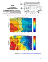
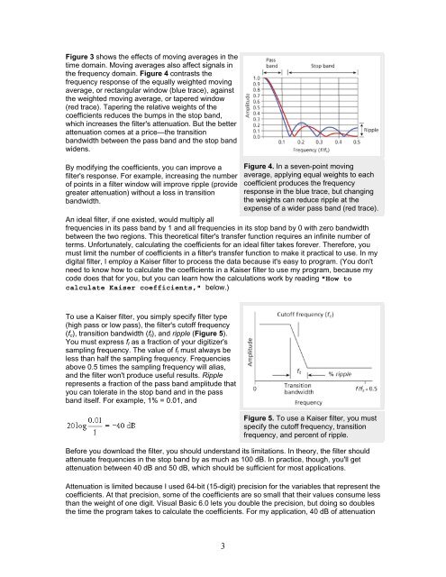
Figure 3 shows the effects of moving averages in the
time domain. Moving averages also affect signals in
the frequency domain. Figure 4 contrasts the
frequency response of the equally weighted moving
average, or rectangular window (blue trace), against
the weighted moving average, or tapered window
(red trace). Tapering the relative weights of the
coefficients reduces the bumps in the stop band,
which increases the filter's attenuation. But the better
attenuation comes at a price—the transition
bandwidth between the pass band and the stop band
widens.
By modifying the coefficients, you can improve a
filter's response. For example, increasing the number
of points in a filter window will improve ripple (provide
greater attenuation) without a loss in transition
bandwidth.
Figure 4. In a seven-point moving
average, applying equal weights to each
coefficient produces the frequency
response in the blue trace, but changing
the weights can reduce ripple at the
expense of a wider pass band (red trace).
An ideal filter, if one existed, would multiply all
frequencies in its pass band by 1 and all frequencies in its stop band by 0 with zero bandwidth
between the two regions. This theoretical filter's transfer function requires an infinite number of
terms. Unfortunately, calculating the coefficients for an ideal filter takes forever. Therefore, you
must limit the number of coefficients in a filter's transfer function to make it practical to use. In my
digital filter, I employ a Kaiser filter to process the data because it's easy to program. (You don't
need to know how to calculate the coefficients in a Kaiser filter to use my program, because my
code does that for you, but you can learn how the calculations work by reading "How to
calculate Kaiser coefficients," below.)
To use a Kaiser filter, you simply specify filter type
(high pass or low pass), the filter's cutoff frequency
(f c ), transition bandwidth (f t ), and ripple (Figure 5).
You must express f t as a fraction of your digitizer's
sampling frequency. The value of f t must always be
less than half the sampling frequency. Frequencies
above 0.5 times the sampling frequency will alias,
and the filter won't produce useful results. Ripple
represents a fraction of the pass band amplitude that
you can tolerate in the stop band and in the pass
band itself. For example, 1% = 0.01, and
Figure 5. To use a Kaiser filter, you must
specify the cutoff frequency, transition
frequency, and percent of ripple.
Before you download the filter, you should understand its limitations. In theory, the filter should
attenuate frequencies in the stop band by as much as 100 dB. In practice, though, you'll get
attenuation between 40 dB and 50 dB, which should be sufficient for most applications.
Attenuation is limited because I used 64-bit (15-digit) precision for the variables that represent the
coefficients. At that precision, some of the coefficients are so small that their values consume less
than the weight of one digit. Visual Basic 6.0 lets you double the precision, but doing so doubles
the time the program takes to calculate the coefficients. For my application, 40 dB of attenuation
3