The Finite Element Method for the Analysis of Non-Linear and ...
The Finite Element Method for the Analysis of Non-Linear and ...
The Finite Element Method for the Analysis of Non-Linear and ...

Create successful ePaper yourself
Turn your PDF publications into a flip-book with our unique Google optimized e-Paper software.
<strong>The</strong> <strong>Finite</strong> <strong>Element</strong> <strong>Method</strong> <strong>for</strong> <strong>the</strong> <strong>Analysis</strong> <strong>of</strong><br />
<strong>Non</strong>-<strong>Linear</strong> <strong>and</strong> Dynamic Systems<br />
Pr<strong>of</strong>. Dr. Eleni Chatzi<br />
Lecture 6 - 5 November, 2012<br />
Institute <strong>of</strong> Structural Engineering <strong>Method</strong> <strong>of</strong> <strong>Finite</strong> <strong>Element</strong>s II 1
2D Axisymmetric, Plane Strain <strong>and</strong> Plane Stress <strong>Element</strong>s<br />
<strong>The</strong> nodal point coordinates determine <strong>the</strong> spatial configuration <strong>of</strong> <strong>the</strong><br />
element at time 0 <strong>and</strong> t using:<br />
n∑<br />
n∑<br />
0 x 1 (r) = N 0 k x k 1<br />
0 x 2 (r) = N 0 k x k 2<br />
<strong>and</strong> t x 1 (r) =<br />
k=1<br />
n∑<br />
N t k x k 1<br />
k=1<br />
t x 2 (r) =<br />
k=1<br />
n∑<br />
N t k x k 2<br />
k=1<br />
Isoparametric <strong>Element</strong>s ⇒ t u i (r) = ∑ n<br />
k=1 N t k uk i , i=1,2<br />
Institute <strong>of</strong> Structural Engineering <strong>Method</strong> <strong>of</strong> <strong>Finite</strong> <strong>Element</strong>s II 2
2D Axisymmetric, Plane Strain <strong>and</strong> Plane Stress <strong>Element</strong>s<br />
Shape Functions<br />
n = 4 nodes<br />
N1 a = 1 4 (1 + r)(1 + s), N 2 a = 1 4 (1 − r)(1 + s), N 3 a = 1 (1 − r)(1 − s),<br />
4<br />
N4 a = 1 (1 + r)(1 − s)<br />
4<br />
n = 8 nodes<br />
N b 5 = 1 2 (1 − r2 )(1 + s), N b 6 = 1 2 (1 − s2 )(1 − r), N b 7 = 1 2 (1 − r2 )(1 − s),<br />
N b 8 = 1 2 (1 − s2 )(1 + r)<br />
N b 1 = N a 1 − 1 2 N b 5 − 1 2 N b 8 , N b 2 = N a 2 − 1 2 N b 6 − 1 2 N b 7 , N b 3 = N a 3 − 1 2 N b 6 − 1 2 N b 7 ,<br />
N4 b = N 4 a − 1 2 N 7 b − 1 2 N 8<br />
b<br />
n = 9 nodes<br />
N9 c = (1 − r2 )(1 − s 2 ),<br />
Ni c = N i b − 1 4 N 9 c, i=1,2,3,4<br />
Nj c = N j b − 1 2 N 9 c, i=5,6,7,8<br />
Institute <strong>of</strong> Structural Engineering <strong>Method</strong> <strong>of</strong> <strong>Finite</strong> <strong>Element</strong>s II 3
2D Axisymmetric, Plane Strain <strong>and</strong> Plane Stress <strong>Element</strong>s<br />
Institute <strong>of</strong> Structural Engineering <strong>Method</strong> <strong>of</strong> <strong>Finite</strong> <strong>Element</strong>s II 4
2D Axisymmetric, Plane Strain <strong>and</strong> Plane Stress <strong>Element</strong>s<br />
Institute <strong>of</strong> Structural Engineering <strong>Method</strong> <strong>of</strong> <strong>Finite</strong> <strong>Element</strong>s II 5
2D Axisymmetric, Plane Strain <strong>and</strong> Plane Stress <strong>Element</strong>s<br />
Institute <strong>of</strong> Structural Engineering <strong>Method</strong> <strong>of</strong> <strong>Finite</strong> <strong>Element</strong>s II 6
2D Axisymmetric, Plane Strain <strong>and</strong> Plane Stress <strong>Element</strong>s<br />
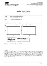
Example<br />
Establish <strong>the</strong> Total Lagrangian Strain - Displacement matrices <strong>for</strong><br />
<strong>the</strong> following element (assuming large displacements/large strains):<br />
Institute <strong>of</strong> Structural Engineering <strong>Method</strong> <strong>of</strong> <strong>Finite</strong> <strong>Element</strong>s II 7
2D Axisymmetric, Plane Strain <strong>and</strong> Plane Stress <strong>Element</strong>s<br />
Example<br />
<strong>The</strong> nodal coordinates at time<br />
t are:<br />
t<br />
u 1 2=0.5<br />
t<br />
u 1 1= 1<br />
t u 1 1 = 1<br />
t u 2 1 = 0<br />
t u 3 1 = 0<br />
t u 4 1 = 1<br />
t u 1 2 = 0.5<br />
t u 2 2 = 0.5<br />
t u 3 2 = 0<br />
t u 4 2 = 0<br />
<strong>The</strong> Jacobian <strong>for</strong> a 2D system is defined as:<br />
009 Example 6.18<br />
7<br />
⎡<br />
⎤ ⎡ ⎤<br />
0 J =<br />
⎢<br />
⎣<br />
∂ t x 1<br />
∂r<br />
∂ t x 1<br />
∂s<br />
∂ t x 2<br />
∂r<br />
∂ t x 2<br />
∂s<br />
⎥<br />
⎦ =<br />
⎢<br />
⎣<br />
3<br />
2<br />
0<br />
0<br />
3<br />
2<br />
⎥<br />
⎦<br />
Institute <strong>of</strong> Structural Engineering <strong>Method</strong> <strong>of</strong> <strong>Finite</strong> <strong>Element</strong>s II 8
2D Axisymmetric, Plane Strain <strong>and</strong> Plane Stress <strong>Element</strong>s<br />
Example - <strong>Linear</strong> Strain Displacement Matrix component t 0B L0<br />
Using <strong>the</strong> 4 node 2D element shape functions <strong>and</strong> <strong>the</strong> relevant<br />
matrix we obtain:<br />
Institute <strong>of</strong> Structural Engineering <strong>Method</strong> <strong>of</strong> <strong>Finite</strong> <strong>Element</strong>s II 9
2D Axisymmetric, Plane Strain <strong>and</strong> Plane Stress <strong>Element</strong>s<br />
Example - <strong>Non</strong>linear Strain Displacement Matrix component t 0B L1<br />
We first need to calculate <strong>the</strong> following terms:<br />
Institute <strong>of</strong> Structural Engineering <strong>Method</strong> <strong>of</strong> <strong>Finite</strong> <strong>Element</strong>s II 10
2D Axisymmetric, Plane Strain <strong>and</strong> Plane Stress <strong>Element</strong>s<br />
Example - <strong>Linear</strong> Strain Displacement Matrix component t 0B L1<br />
Institute <strong>of</strong> Structural Engineering <strong>Method</strong> <strong>of</strong> <strong>Finite</strong> <strong>Element</strong>s II 11
2D Axisymmetric, Plane Strain <strong>and</strong> Plane Stress <strong>Element</strong>s<br />
Example - <strong>Non</strong>linear Strain Displacement Matrix component t 0B NL<br />
Using <strong>the</strong> 4 node 2D element shape functions <strong>and</strong> <strong>the</strong> relevant matrix we<br />
obtain:<br />
Institute <strong>of</strong> Structural Engineering <strong>Method</strong> <strong>of</strong> <strong>Finite</strong> <strong>Element</strong>s II 12
<strong>The</strong> Beam <strong>Element</strong><br />
*<strong>The</strong> section on <strong>the</strong> Beam <strong>Element</strong> is taken from Pr<strong>of</strong>. H. Waisman’s<br />
notes <strong>of</strong> <strong>the</strong> FEM II course - CEEM Department, Columbia University<br />
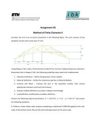
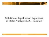
F-16 Aeroelastic Structural Model<br />
Exterior<br />
model<br />
95% are<br />
shell<br />
elements<br />
FEM model:<br />
150000 Nodes<br />
Internal structure<br />
zoom. Some Brick<br />
<strong>and</strong> tetrahedral<br />
elements<br />
http://www.colorado.edu/engineering/CAS/Felippa.d/FelippaHome.d/Home.html<br />
Institute <strong>of</strong> Structural Engineering <strong>Method</strong> <strong>of</strong> <strong>Finite</strong> <strong>Element</strong>s II 13
Beam <strong>Element</strong>s<br />
Two main beam <strong>the</strong>ories:<br />
Euler-Bernoulli <strong>the</strong>ory (Engineering beam <strong>the</strong>ory) -slender beams<br />
Timoshenko <strong>the</strong>ory thick beams<br />
Euler - Bernoulli Beam<br />
Institute <strong>of</strong> Structural Engineering <strong>Method</strong> <strong>of</strong> <strong>Finite</strong> <strong>Element</strong>s II 14
Beam <strong>Element</strong>s<br />
Euler Bernoulli Beam Assumptions - Kirchh<strong>of</strong>f Assumptions<br />
Normals remain straight (<strong>the</strong>y do not bend)<br />
Normals remain unstretched (<strong>the</strong>y keep <strong>the</strong> same length)<br />
Normals remain normal (<strong>the</strong>y always make a right angle to <strong>the</strong> neutral<br />
plane)<br />
Institute <strong>of</strong> Structural Engineering <strong>Method</strong> <strong>of</strong> <strong>Finite</strong> <strong>Element</strong>s II 15
Beam <strong>Element</strong>s - Strong Form<br />
υ´ υ´<br />
υ<br />
Institute <strong>of</strong> Structural Engineering <strong>Method</strong> <strong>of</strong> <strong>Finite</strong> <strong>Element</strong>s II 16
Beam <strong>Element</strong>s - Strong Form<br />
Equilibrium<br />
– distributed load per unit length<br />
– shear <strong>for</strong>ce<br />
Combining <strong>the</strong> equations<br />
Institute <strong>of</strong> Structural Engineering <strong>Method</strong> <strong>of</strong> <strong>Finite</strong> <strong>Element</strong>s II 17
Beam <strong>Element</strong>s - Strong Form<br />
(1)<br />
Free end with applied load<br />
(2)<br />
(S)<br />
(3)<br />
Simple support<br />
(4)<br />
(5)<br />
Clamped support<br />
Institute <strong>of</strong> Structural Engineering <strong>Method</strong> <strong>of</strong> <strong>Finite</strong> <strong>Element</strong>s II 18
Beam <strong>Element</strong>s - Strong Form to Weak Form<br />
Multiply Eqns. Multiply (1), Eq. (4) (1), (5) by (4) w(5) <strong>and</strong> by integrate w <strong>and</strong> integrate over <strong>the</strong>over domain <strong>the</strong> domain<br />
First integration by parts<br />
First integration by parts<br />
First integration First integration by parts by parts<br />
Second integration by parts gives<br />
Second integration by parts gives<br />
Second integration by parts gives<br />
Second integration by parts gives<br />
Institute <strong>of</strong> Structural Engineering <strong>Method</strong> <strong>of</strong> <strong>Finite</strong> <strong>Element</strong>s II 19
Beam <strong>Element</strong>s - Strong Form to Weak Form<br />
Arrive at <strong>the</strong> weak <strong>for</strong>m<br />
(W)<br />
Note:<br />
1. <strong>The</strong> spaces are C 1 continuous, i.e. <strong>the</strong> derivative must also be<br />
continuous<br />
Note:<br />
1. <strong>The</strong> spaces are C 1 continuous, i.e. <strong>the</strong> derivative must also be<br />
continuous<br />
2. <strong>The</strong> left side is symmetric in w <strong>and</strong> υ (bi-linear <strong>for</strong>m:<br />
a(υ, w)=a(w, υ)) this will lead to a symmetric Stiffness Matrix<br />
2. <strong>The</strong> left side is symmetric in w <strong>and</strong> v (bi-linear <strong>for</strong>m: a(v,w)=a(w,v)<br />
this will lead to symmetric stiffness matrix<br />
Institute <strong>of</strong> Structural Engineering <strong>Method</strong> <strong>of</strong> <strong>Finite</strong> <strong>Element</strong>s II 20
Beam <strong>Element</strong>s - FE Formulation<br />
Physical domain<br />
Natural domain<br />
<strong>Element</strong><br />
displacement<br />
vector<br />
<strong>Element</strong><br />
<strong>for</strong>ce<br />
vector<br />
Institute <strong>of</strong> Structural Engineering <strong>Method</strong> <strong>of</strong> <strong>Finite</strong> <strong>Element</strong>s II 21
Beam <strong>Element</strong>s - Shape Functions<br />
Hermite<br />
Hermite<br />
Polynomials<br />
Polynomials<br />
Note: <strong>The</strong> choice <strong>of</strong> a cubic polynomial is related to <strong>the</strong> homogeneous<br />
strong <strong>for</strong>m <strong>of</strong> <strong>the</strong> problem EIυ ′′′′ = 0.<br />
Institute <strong>of</strong> Structural Engineering <strong>Method</strong> <strong>of</strong> <strong>Finite</strong> <strong>Element</strong>s II 22
Beam <strong>Element</strong>s - Shape Functions<br />
<strong>The</strong> displacement is approximated by<br />
However note :<br />
From coordinate trans<strong>for</strong>mation (mapping)<br />
Institute <strong>of</strong> Structural Engineering <strong>Method</strong> <strong>of</strong> <strong>Finite</strong> <strong>Element</strong>s II 23
Beam <strong>Element</strong>s - Galerkin<br />
Finally, <strong>the</strong> weight functions <strong>and</strong> trial solutions are<br />
Finally, <strong>the</strong> weight functions <strong>and</strong> trial solutions<br />
Where <strong>the</strong> shape functions are<br />
Institute <strong>of</strong> Structural Engineering <strong>Method</strong> <strong>of</strong> <strong>Finite</strong> <strong>Element</strong>s II 24
Beam <strong>Element</strong>s - FE Matrices<br />
From<br />
From<br />
<strong>the</strong> weak<br />
<strong>the</strong><br />
<strong>for</strong>m,<br />
weak<br />
we<br />
<strong>for</strong>m,<br />
had<br />
we had<br />
<strong>The</strong> second <strong>The</strong> second derivative derivative becomes becomes<br />
<strong>and</strong><br />
Institute <strong>of</strong> Structural Engineering <strong>Method</strong> <strong>of</strong> <strong>Finite</strong> <strong>Element</strong>s II 25
Beam <strong>Element</strong>s - FE Matrices<br />
Stiffness matrix<br />
Force vector<br />
Assuming constant distributed <strong>for</strong>ce<br />
Institute <strong>of</strong> Structural Engineering <strong>Method</strong> <strong>of</strong> <strong>Finite</strong> <strong>Element</strong>s II 26
Beam <strong>Element</strong>s - Example<br />
Consider a clamped-free beam<br />
with EI = 10 4 Nm 2<br />
s = −20N<br />
m = 20Nm<br />
Consider a clamped-free beam<br />
Pre-processing<br />
Institute <strong>of</strong> Structural Engineering <strong>Method</strong> <strong>of</strong> <strong>Finite</strong> <strong>Element</strong>s II 27
Beam <strong>Element</strong>s - Example<br />
For element (1) For element (2)<br />
[1] [2] [3] [4] [3] [4] [5] [6]<br />
Assembly into a Global Stiffness Matrix<br />
Institute <strong>of</strong> Structural Engineering <strong>Method</strong> <strong>of</strong> <strong>Finite</strong> <strong>Element</strong>s II 28
Beam <strong>Element</strong>s - Example<br />
Boundary <strong>for</strong>ce matrix<br />
<strong>Element</strong> (1) has no boundary on Γ S or Γ M<br />
For element (2) we have<br />
[3]<br />
[4]<br />
[5]<br />
[6]<br />
Assembly to global boundary <strong>for</strong>ce vector<br />
Institute <strong>of</strong> Structural Engineering <strong>Method</strong> <strong>of</strong> <strong>Finite</strong> <strong>Element</strong>s II 29
Beam <strong>Element</strong>s - Example<br />
Body <strong>for</strong>ce vector<br />
(distributed<br />
loads)<br />
(Point loads)<br />
For element (1) Given:<br />
For element (2) Given:<br />
Institute <strong>of</strong> Structural Engineering <strong>Method</strong> <strong>of</strong> <strong>Finite</strong> <strong>Element</strong>s II 30
Beam <strong>Element</strong>s - Example<br />
<strong>The</strong> global <strong>for</strong>ce vector<br />
-9<br />
-15.3<br />
-4<br />
15.3<br />
-20<br />
20<br />
=KNOWN<br />
Post-processing<br />
Institute <strong>of</strong> Structural Engineering <strong>Method</strong> <strong>of</strong> <strong>Finite</strong> <strong>Element</strong>s II 31
Timoshenko Beam<br />
In a Timoshenko Beam, a plane normal to<br />
<strong>the</strong> beam axis be<strong>for</strong>e de<strong>for</strong>mation doesnt<br />
remain normal after de<strong>for</strong>mation (short <strong>and</strong><br />
thick beams, s<strong>and</strong>wich composite beams).<br />
i.e. θ ≠ dv<br />
dx :<br />
γ = −θ + dv Transverse Shear strain<br />
dx<br />
ε = −y dθ Normal strain<br />
dx<br />
<strong>The</strong> strain energy <strong>of</strong> an element may be written as<br />
G - shear modulus<br />
b - widthh<br />
µ - correction factor<br />
h - height<br />
Institute <strong>of</strong> Structural Engineering <strong>Method</strong> <strong>of</strong> <strong>Finite</strong> <strong>Element</strong>s II 32
Timoshenko Beam<br />
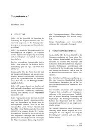
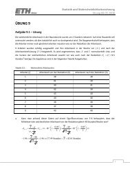
Chapter 9: THE TL TIMOSHENKO PLANE BEAM ELEMENT 9–8<br />
2-node C 1 (cubic) element<br />
<strong>for</strong> Euler-Bernoulli beam model:<br />
plane sections remain plane <strong>and</strong><br />
normal to de<strong>for</strong>med longitudinal axis<br />
2-node C 0 linear-displacement-<strong>and</strong>-rotations<br />
element <strong>for</strong> Timoshenko beam model:<br />
plane sections remain plane but not<br />
normal to de<strong>for</strong>med longitudinal axis<br />
(a)<br />
(b)<br />
C 1 element<br />
with same DOFs<br />
Figure 9.6. Sketch <strong>of</strong> <strong>the</strong> kinematics <strong>of</strong> two-node beam finite element models based on<br />
(a) Euler-Bernoulli beam <strong>the</strong>ory, <strong>and</strong> (b) Timoshenko beam <strong>the</strong>ory. <strong>The</strong>se<br />
models are called C 1 <strong>and</strong> C 0 beams, respectively, in <strong>the</strong> FEM literature.<br />
Institute <strong>of</strong> Structural Engineering <strong>Method</strong> <strong>of</strong> <strong>Finite</strong> <strong>Element</strong>s II 33
Timoshenko Beam<br />
Substituting <strong>the</strong> relations into U<br />
Substituting <strong>the</strong> relations into U<br />
Substituting <strong>the</strong> relations into U<br />
I - moment <strong>of</strong> inertia<br />
I -moment - A -<strong>of</strong> <strong>of</strong> cross-sectional inertia, A-cross-sectional area area<br />
A<br />
- cross-sectional area<br />
Galerkins<br />
Galerkin’s<br />
Approximation<br />
Approximation<br />
(<strong>Linear</strong><br />
(<strong>Linear</strong><br />
shape<br />
shape<br />
functions)<br />
functions)<br />
Galerkin’s Approximation (<strong>Linear</strong> shape functions)<br />
<strong>Element</strong> stiffness<br />
<strong>Element</strong> stiffness<br />
<strong>Element</strong> stiffness<br />
Institute <strong>of</strong> Structural Engineering <strong>Method</strong> <strong>of</strong> <strong>Finite</strong> <strong>Element</strong>s II 34
Timoshenko Beam<br />
Exact integration<br />
Shear Locking<br />
Example: Cantilever Beam,<br />
20 elements, different<br />
span L to depth h<br />
Reduced 1-point quadrature integration<br />
Ratio <strong>of</strong> tip displacement <strong>for</strong><br />
Timoshenko beam <strong>the</strong>ory <strong>and</strong><br />
Euler-Bernoulli <strong>the</strong>ory<br />
Institute <strong>of</strong> Structural Engineering <strong>Method</strong> <strong>of</strong> <strong>Finite</strong> <strong>Element</strong>s II 35
Timoshenko Beam<br />
<strong>The</strong> Shear locking Phenomenon<br />
This occurs when significant bending is present. It is owed to <strong>the</strong> use<br />
<strong>of</strong> linear shape functions that cannot accurately model <strong>the</strong> curvature<br />
that is present in <strong>the</strong> actual material under bending condition.<br />
Instead, a shear stress is introduced which causes <strong>the</strong> element to<br />
reach equilibrium conditions <strong>for</strong> smaller displacements that <strong>the</strong> real<br />
ones.<br />
<strong>The</strong> element <strong>the</strong>re<strong>for</strong>e appears stiffer.<br />
Institute <strong>of</strong> Structural Engineering <strong>Method</strong> <strong>of</strong> <strong>Finite</strong> <strong>Element</strong>s II 36
<strong>The</strong> Beam <strong>Element</strong> in Large Displacements<br />
Assumptions:<br />
Plane sections initially normal to <strong>the</strong> neutral axis remain plane<br />
<strong>The</strong> longitudinal (ε ηη) <strong>and</strong> <strong>the</strong> two shear stresses(ε ηξ , ε ηζ ) are <strong>the</strong> only non<br />
zero ones.<br />
A general 3D beam element would <strong>the</strong>n be:<br />
Institute <strong>of</strong> Structural Engineering <strong>Method</strong> <strong>of</strong> <strong>Finite</strong> <strong>Element</strong>s II 37
<strong>The</strong> Beam <strong>Element</strong> in Large Displacements<br />
Along <strong>the</strong> lines <strong>of</strong> <strong>the</strong> truss element <strong>for</strong>mulation we need to express <strong>the</strong><br />
coordinates <strong>of</strong> a r<strong>and</strong>om point within <strong>the</strong> beam element. Using (r, s, t) as<br />
<strong>the</strong> Cartesian coordinates at a point within an element with N nodal<br />
points, this is written:<br />
t x i =<br />
N∑<br />
N t k x k i + t 2<br />
k=1<br />
N∑<br />
k=1<br />
a k N k t V k<br />
ti + s 2<br />
N∑<br />
k=1<br />
b k N k t V k<br />
si, i = 1, 2, 3<br />
Vectors V s <strong>and</strong> V t define <strong>the</strong> orientation <strong>of</strong> <strong>the</strong> cross-section <strong>for</strong> <strong>the</strong> beam:<br />
<strong>The</strong>y are normal to <strong>the</strong> axis <strong>of</strong> <strong>the</strong> beam <strong>and</strong> to each o<strong>the</strong>r. <strong>The</strong> values a<br />
<strong>and</strong> b define <strong>the</strong> size <strong>of</strong> <strong>the</strong> cross section <strong>of</strong> <strong>the</strong> beam.<br />
<strong>The</strong> relative displacement components would be:<br />
t u i = t x i − 0 x i<br />
u i = t + ∆ t x i − t x i<br />
are <strong>the</strong> incremental components<br />
Institute <strong>of</strong> Structural Engineering <strong>Method</strong> <strong>of</strong> <strong>Finite</strong> <strong>Element</strong>s II 38
<strong>The</strong> Beam <strong>Element</strong> in Large Displacements<br />
This leads to <strong>the</strong> following <strong>for</strong>mulations<br />
t<br />
u i =<br />
N∑<br />
N kt u k i + t 2<br />
k=1<br />
N∑<br />
k=1<br />
a k N k ( t V k<br />
ti − 0 V k ti) + s 2<br />
N∑<br />
k=1<br />
b k N k ( t V k si − 0 V k<br />
si)<br />
<strong>and</strong> u i =<br />
where<br />
N∑<br />
N k u k i + t 2<br />
k=1<br />
N∑<br />
k=1<br />
a k N k V k<br />
ti + s 2<br />
N∑<br />
k=1<br />
Vti k = t + ∆ t Vti k − t Vti<br />
k<br />
Vsi k = t + ∆ t Vsi k − t Vsi<br />
k<br />
b k N k V k<br />
si, i = 1, 2, 3<br />
Institute <strong>of</strong> Structural Engineering <strong>Method</strong> <strong>of</strong> <strong>Finite</strong> <strong>Element</strong>s II 39
<strong>The</strong> Beam <strong>Element</strong> in Large Displacements<br />
We need to express <strong>the</strong> components V k<br />
ti , ZV k<br />
si <strong>of</strong> <strong>the</strong> vectors Vk t , V k s in<br />
terms <strong>of</strong> <strong>the</strong> nodal rotational degrees <strong>of</strong> freedom per node k:<br />
θ T k = [ θ k x θ k y θ k z<br />
This in linear analysis would be written as:<br />
V k t = θ k × t V k t<br />
V k s = θ k × t V k s<br />
but in <strong>the</strong> case <strong>of</strong> large displacements a second order Taylor approximation<br />
needs to be used:<br />
V k t = θ k × t V k t + 1 2 θ k × (θ k × t V k t )<br />
V k s = θ k × t V k s + 1 2 θ k × (θ k × t V k s)<br />
]<br />
Institute <strong>of</strong> Structural Engineering <strong>Method</strong> <strong>of</strong> <strong>Finite</strong> <strong>Element</strong>s II 40
<strong>The</strong> Beam <strong>Element</strong> in Large Displacements<br />
<strong>The</strong> finite element equations in this case are:<br />
t K<br />
⎡<br />
⎢<br />
⎣<br />
.<br />
u k<br />
θ k<br />
.<br />
⎤<br />
⎥<br />
⎦ = t + ∆t R − t F (1)<br />
Having solved Eqn (1) <strong>for</strong> bfu k , θ k , we obtain <strong>the</strong> approximations <strong>for</strong> <strong>the</strong><br />
nodal point displacement <strong>and</strong> direction vectors:<br />
t + ∆t u k = t u k + u<br />
∫ k<br />
t + ∆t V k t = t Vt k + dθ k × τ Vt<br />
k<br />
V<br />
∫ k<br />
t + ∆t V k s = t Vs k + dθ k × τ Vs<br />
k<br />
V k<br />
<strong>The</strong> above <strong>for</strong>mulation corresponds to an iteration <strong>of</strong> <strong>the</strong> Newton-Raphson<br />
method<br />
Institute <strong>of</strong> Structural Engineering <strong>Method</strong> <strong>of</strong> <strong>Finite</strong> <strong>Element</strong>s II 41
<strong>The</strong> Beam <strong>Element</strong> in Large Displacements<br />
Example:<br />
Assume <strong>the</strong> following 2-node beam element. Evaluate <strong>the</strong> coordinate <strong>and</strong><br />
displacement interpolations <strong>and</strong> derivatives required <strong>for</strong> <strong>the</strong> setup <strong>of</strong> <strong>the</strong><br />
strain displacement matrices in <strong>the</strong> TL <strong>and</strong> UL <strong>for</strong>mulation.<br />
Institute <strong>of</strong> Structural Engineering <strong>Method</strong> <strong>of</strong> <strong>Finite</strong> <strong>Element</strong>s II 42
<strong>The</strong> Beam <strong>Element</strong> in Large Displacements<br />
Example:<br />
First we need to calculate <strong>the</strong> nodal coordinates at times t <strong>and</strong> 0 ( t x 1 , t x 2 ),<br />
( 0 x 1 , 0 x 2 ). Using <strong>the</strong> corresponding geometries <strong>and</strong> <strong>the</strong> following <strong>for</strong>mula:<br />
t x i =<br />
N∑<br />
N t k x k i + t 2<br />
k=1<br />
N∑<br />
k=1<br />
a k N k t V k<br />
ti + s 2<br />
N∑<br />
k=1<br />
where N k are linear shape functions, we obtain:<br />
b k N k t V k<br />
si, i = 1, 2, 3<br />
Institute <strong>of</strong> Structural Engineering <strong>Method</strong> <strong>of</strong> <strong>Finite</strong> <strong>Element</strong>s II 43
<strong>The</strong> Beam <strong>Element</strong> in Large Displacements<br />
Example:<br />
Hence, <strong>the</strong> displacement components are at time t given by <strong>the</strong> following<br />
<strong>for</strong>mula:<br />
N∑<br />
t u i = N t k u k i + t N∑<br />
a k N k ( t Vti k − 0 Vti) k + s 2<br />
2<br />
k=1<br />
k=1<br />
N∑<br />
k=1<br />
b k N k ( t V k si − 0 V k<br />
si), i = 1, 2<br />
hence:<br />
Institute <strong>of</strong> Structural Engineering <strong>Method</strong> <strong>of</strong> <strong>Finite</strong> <strong>Element</strong>s II 44
<strong>The</strong> Beam <strong>Element</strong> in Large Displacements<br />
Example:<br />
For <strong>the</strong> calculation <strong>of</strong> <strong>the</strong> incremental displacements we will need to<br />
calculate <strong>the</strong> rotational components V s t (since V k t = 0). Using <strong>the</strong><br />
following <strong>for</strong>mula:<br />
V k s = θ k × t V k s + 1 2 θ k × (θ k × t V k s)<br />
we get:<br />
θ k × t V k s =<br />
∣<br />
e 1 e 2 e 3<br />
0 0 θ<br />
−sin( t θ k ) cos( t θ k ) 0<br />
⎡<br />
∣ = ⎣<br />
−θ k cos( t θ k )<br />
−θ k sin( t θ k )<br />
0<br />
⎤<br />
⎦<br />
<strong>and</strong> θ k × (θ k × t V k s) =<br />
∣<br />
e 1 e 2 e 3<br />
0 0 θ<br />
−θ k cos( t θ k ) −θ k sin( t θ k ) 0<br />
⎡<br />
∣ = ⎣<br />
θ 2 k sin(t θ k )<br />
−θ 2 k cos(t θ k )<br />
0<br />
⎤<br />
⎦<br />
Institute <strong>of</strong> Structural Engineering <strong>Method</strong> <strong>of</strong> <strong>Finite</strong> <strong>Element</strong>s II 45
<strong>The</strong> Beam <strong>Element</strong> in Large Displacements<br />
Example:<br />
<strong>The</strong>n, <strong>the</strong> incremental displacements are given by<br />
<strong>and</strong> u i =<br />
N∑<br />
N k u k i + t 2<br />
k=1<br />
N∑<br />
k=1<br />
a k N k V k<br />
ti + s 2<br />
N∑<br />
k=1<br />
b k N k V k<br />
si, i = 1, 2<br />
hence:<br />
Institute <strong>of</strong> Structural Engineering <strong>Method</strong> <strong>of</strong> <strong>Finite</strong> <strong>Element</strong>s II 46
<strong>The</strong> Beam <strong>Element</strong> in Large Displacements<br />
Example:<br />
Finally, <strong>the</strong> required derivatives <strong>for</strong> <strong>the</strong> TL <strong>and</strong> UL <strong>for</strong>mulation will be:<br />
where we assumed t L = 0 L = L.<br />
Institute <strong>of</strong> Structural Engineering <strong>Method</strong> <strong>of</strong> <strong>Finite</strong> <strong>Element</strong>s II 47
<strong>The</strong> Beam <strong>Element</strong> in Large Displacements<br />
Example:<br />
Also, <strong>the</strong> Jacobian will be:<br />
And <strong>the</strong> associated displacement derivatives are:<br />
<strong>The</strong>se will be used to derive <strong>the</strong> strain-displacement matrices B <strong>and</strong> finally <strong>the</strong><br />
stiffness matrix K<br />
Institute <strong>of</strong> Structural Engineering <strong>Method</strong> <strong>of</strong> <strong>Finite</strong> <strong>Element</strong>s II 48
Special Considerations-Geometric Stiffness<br />
An alternate approach to <strong>the</strong> Large Displacement Problem <strong>for</strong> practical<br />
considerations (namely truss, beam problems)<br />
A cable, when subjected to a large tension <strong>for</strong>ce, has an increased lateral stiffness.<br />
If a long rod is subjected to a large compressive <strong>for</strong>ce, <strong>and</strong> is on <strong>the</strong> verge <strong>of</strong><br />
buckling, we know that <strong>the</strong> lateral stiffness <strong>of</strong> <strong>the</strong> rod has been reduced<br />
significantly <strong>and</strong> a small lateral load may cause <strong>the</strong> rod to buckle. This general<br />
type <strong>of</strong> behavior is caused by a change in <strong>the</strong> “geometric stiffness <strong>of</strong> <strong>the</strong><br />
structure. This stiffness is a function <strong>of</strong> <strong>the</strong> load in <strong>the</strong> structural member <strong>and</strong><br />
can be ei<strong>the</strong>r positive or negative.<br />
Institute <strong>of</strong> Structural Engineering <strong>Method</strong> <strong>of</strong> <strong>Finite</strong> <strong>Element</strong>s II 49
Special Considerations-Geometric Stiffness<br />
Cable <strong>Element</strong><br />
<strong>The</strong> fundamental equations <strong>for</strong> <strong>the</strong> geometric stiffness <strong>for</strong> a rod or a cable are<br />
very simple to derive. Consider <strong>the</strong> horizontal cable, <strong>of</strong> length L with an initial<br />
tension T. If <strong>the</strong> cable is subjected to lateral displacements, v i <strong>and</strong> v j , at both<br />
DYNAMIC ANALYSIS OF STRUCTURES<br />
ends, as shown, <strong>the</strong>n additional <strong>for</strong>ces, F i <strong>and</strong> F j , must be developed <strong>for</strong> <strong>the</strong><br />
cable element to be in equilibrium in its displaced position.<br />
T<br />
Fi<br />
´<br />
De<strong>for</strong>med Position<br />
F j<br />
T<br />
v i<br />
´<br />
i<br />
L<br />
´<br />
´<br />
j<br />
v j<br />
T<br />
T<br />
Note that we haveFigure assumed 11.1. all <strong>for</strong>ces Forces <strong>and</strong>Acting displacements on a Cable are positive <strong>Element</strong> in <strong>the</strong> up<br />
direction. We have also made <strong>the</strong> assumption that <strong>the</strong> displacements are small<br />
Taking <strong>and</strong> do not moments changeabout <strong>the</strong> tension point j in in <strong>the</strong> <strong>the</strong> cable. de<strong>for</strong>med position, <strong>the</strong> following equilibrium<br />
equation can be written:<br />
Institute <strong>of</strong> Structural Engineering <strong>Method</strong> <strong>of</strong> <strong>Finite</strong> <strong>Element</strong>s II 50
Special Considerations-Geometric Stiffness<br />
Taking moments about point j in <strong>the</strong> de<strong>for</strong>med position, <strong>the</strong> following<br />
equilibrium equation can be written:<br />
F i = T (vi − vj)<br />
L<br />
And from vertical equilibrium <strong>the</strong> following equation is apparent:<br />
F i = −F j<br />
Combining <strong>the</strong> above <strong>the</strong> lateral <strong>for</strong>ces can be expressed in terms <strong>of</strong> <strong>the</strong> lateral<br />
displacements by <strong>the</strong> following matrix equation:<br />
[ ]<br />
Fi<br />
= T [ ] [ ]<br />
1 −1 vi<br />
or symbolically, F<br />
F j L −1 1 v G = K Gv<br />
j<br />
Note that <strong>the</strong> 2 × 2 geometric stiffness, K G , matrix is not a function <strong>of</strong> <strong>the</strong> mechanical<br />
properties <strong>of</strong> <strong>the</strong> cable <strong>and</strong> is only a function <strong>of</strong> <strong>the</strong> elements length <strong>and</strong> <strong>the</strong> <strong>for</strong>ce in <strong>the</strong><br />
element. Hence, <strong>the</strong> term “geometric or “stress stiffness matrix is introduced as opposed<br />
to <strong>the</strong> “mechanical stiffness matrix which is based on <strong>the</strong> physical properties. <strong>The</strong><br />
geometric stiffness exists in all structures; however, it only becomes important if it is<br />
large compared to <strong>the</strong> mechanical stiffness <strong>of</strong> <strong>the</strong> structural system.<br />
Institute <strong>of</strong> Structural Engineering <strong>Method</strong> <strong>of</strong> <strong>Finite</strong> <strong>Element</strong>s II 51
Special Considerations-Geometric Stiffness<br />
Beam <strong>Element</strong><br />
In <strong>the</strong> case <strong>of</strong> a beam element with bending properties in which <strong>the</strong> de<strong>for</strong>med<br />
shape is assumed to be a cubic function due to <strong>the</strong> rotations φ i <strong>and</strong> φ j at <strong>the</strong><br />
ends, additional moments M i <strong>and</strong> M j are developed. <strong>The</strong> <strong>for</strong>ce-displacement<br />
relationship is given by <strong>the</strong> following equation:<br />
⎡<br />
⎢<br />
⎣<br />
F i<br />
M i<br />
F j<br />
M j<br />
⎤<br />
⎥<br />
⎦ =<br />
T<br />
30L<br />
⎡<br />
⎢<br />
⎣<br />
⎤<br />
36 3L −36 3L<br />
3L 4L 2 −3L −L 2<br />
⎥<br />
−36 −3L 36 −3L ⎦<br />
3L −L 2 −3L 4L 2<br />
⎡<br />
⎢<br />
⎣<br />
v i<br />
φ i<br />
v j<br />
φ j<br />
⎤<br />
⎥<br />
⎦<br />
or FG = KGv<br />
<strong>The</strong> well-known elastic <strong>for</strong>ce de<strong>for</strong>mation relationship, <strong>for</strong> a prismatic beam<br />
without shearing de<strong>for</strong>mations, is<br />
⎡ ⎤ ⎡<br />
⎤ ⎡ ⎤<br />
F i<br />
12 6L −12 6L v i<br />
⎢ M i<br />
⎥<br />
⎣ F j<br />
⎦ = EI<br />
⎢ 6L 4L 2 −6L −2L 2<br />
⎥ ⎢ φ i<br />
⎥<br />
L 3 ⎣ −12 −6L 12 −6L ⎦ ⎣ v j<br />
⎦ or FE = KEv<br />
M j<br />
−6L −2L 2 −6L 4L 2 φ j<br />
<strong>The</strong>re<strong>for</strong>e, <strong>the</strong> total <strong>for</strong>ces acting on <strong>the</strong> beam element will be:<br />
F T = F E + F G = [K E + K G]v = K T v<br />
Institute <strong>of</strong> Structural Engineering <strong>Method</strong> <strong>of</strong> <strong>Finite</strong> <strong>Element</strong>s II 52
Special Considerations - Geometric Stiffness<br />
Conclusion - Geometric Stiffness<br />
In <strong>the</strong> case <strong>of</strong> constant (dead) loads where T is usually constant <strong>the</strong><br />
calculation <strong>of</strong> <strong>the</strong> large displacement effect <strong>for</strong> cable <strong>and</strong> beam<br />
elements is per<strong>for</strong>med by <strong>the</strong> addition in <strong>the</strong> FEM code <strong>of</strong> an<br />
appropriate extra “geometric” stiffness term.<br />
Institute <strong>of</strong> Structural Engineering <strong>Method</strong> <strong>of</strong> <strong>Finite</strong> <strong>Element</strong>s II 53