The Finite Element Method for the Analysis of Non-Linear and ...

The Finite Element Method for the Analysis of
Non-Linear and Dynamic Systems
Prof. Dr. Eleni Chatzi
Lecture 2 - 2 October, 2012
Institute of Structural Engineering Method of Finite Elements II 1

Non Linear FE - Background and Motivation
Linear Analysis Assumptions
Infinitesimally small displacements
Linearly elastic material
No gaps or overlaps occurring during deformations - The
displacement field is smooth
Nature of Boundary Conditions remains unchanged
Steady State Assumption
No dependence on time
Institute of Structural Engineering Method of Finite Elements II 2

Non Linear FE - Background and Motivation
What kind of problems are not steady state and linear?
Material behaves Nonlinearly
Geometric Nonlinearity (ex. p-∆ effects, follower force)
Contact Problems (Hertzian stress)
Loads vary fast compared to the eigenfrequencies of the
structure
Varying Boundary conditions (ex. freezing of water, welding)
General feature:
Response becomes load path dependent
Institute of Structural Engineering Method of Finite Elements II 3

Non Linear FE - Background and Motivation
What is the added value of being able to assess the Nonlinear
non-steady state response of structures?
Assessing the:
Structural response of structures to extreme events (rock-fall,
earthquake, hurricanes)
Performance (failures and deformations) of soils
Verifying simple models
Institute of Structural Engineering Method of Finite Elements II 4

Non Linear FE - Background and Motivation
Collapse Analysis of the World Trade Center
Institute of Structural Engineering Method of Finite Elements II 5

Non Linear FE - Background and Motivation
Ultimate collapse capacity of jacket structure
Institute of Structural Engineering Method of Finite Elements II 6

Non Linear FE - Background and Motivation
Analysis of soil performance
Institute of Structural Engineering Method of Finite Elements II 7

Non Linear FE - Background and Motivation
Analysis of bridge response
Institute of Structural Engineering Method of Finite Elements II 8

Non Linear FE - Background and Motivation
Steady state problems (Linear/Nonlinear):
The response of the system does not change over time
KU = R
Propagation problems (Linear/Nonlinear):
The response of the system changes over time
MÜ(t) + C ˙U(t) + KU(t) = R(t)
Eigenvalue problems:
No unique solution to the response of the system
Institute of Structural Engineering Method of Finite Elements II 9

Introduction Introduction to Nonlinear to non-linear analysis analysis
Classification of Nonlinear analyses
• Classification of non-linear analyses
Type of analysis Description Typical
formulation used
Materially-nonlinear
only
Large
displacements, large
rotations but small
strains
Large
displacements, large
rotations and large
strains
Displacements and
rotations of fibers
are large; but fiber
extensions and
angle changes
between fibers are
small; stress strain
relationship may be
linear or non-linear
Displacements and
rotations of fibers
are large; fiber
extensions and
angle changes
between fibers may
also be large; stress
strain relationship
may be linear or
non-linear
Infinitesimal
displacements and
strains; stress train
relation is nonlinear
Materiallynonlinear-only
(MNO)
Total Lagrange (TL)
Updated Lagrange
(UL)
Total Lagrange (TL)
Updated Lagrange
(UL)
Stress and strain
measures used
Engineering strain
and stress
Second Piola-
Kirchoff stress,
Green-Lagrange
strain
Cauchy stress,
Almansi strain
Second Piola-
Kirchoff stress,
Green-Lagrange
strain
Cauchy stress,
Logarithmic strain
Method of Finite Elements II
Institute of Structural Engineering Method of Finite Elements II 10

Introduction to Nonlinear analysis
Swiss Federal Institute of Technology Page 21
Linear Elastic
Introduction to non-linear analysis
L
• Classification of non-linear analyses
Δ
P
2
P
2
σ = P / A
ε = σ / E
Δ= ε L
σ
1
E
ε < 0.04
ε
L
Infinitesimal Displacements
Linear elastic (infinitesimal displacements)
Method of Finite Elements II
Institute of Structural Engineering Method of Finite Elements II 11

Introduction to Nonlinear analysis
Swiss Federal Institute of Technology Page 22
Material Nonlinearity only
L
Introduction to non-linear analysis
• Classification of non-linear analyses
Δ
P
2
P
2
σ = P/
A
σ
Y
σ −σY
ε = +
E ET
ε < 0.04
σ
σ Y
1
E
P / A
1
E T
ε
L
Method of Finite Elements II
Materially nonlinear only (infinitesimal
displacements, but nonlinear stress-strain relation)
Infinitesimal Displacements, but Nonlinear Stress Strain relation
Institute of Structural Engineering Method of Finite Elements II 12

Introduction to Nonlinear analysis
Swiss Federal Institute of Technology
Large displacements, small strains
Δ′
y
y′
ε ′
x′
L
L
x
ε ′ < 0.04
Δ= ′ ε ′ L
Linear or Nonlinear material behavior
Institute of Structural Engineering Method of Finite Elements II 13

Introduction to Nonlinear to non-linear analysis analysis
• Classification of non-linear analyses
Large displacements, large strains
Linear or Nonlinear material behavior
Large displacements, large rotations and
Institute of Structural Engineering Method of Finite Elements II 14

Introduction Swiss to Federal Nonlinear Institute of Technology analysis
Introduction to non-linear analysis
Change in BC for displacement
• Classification of non-linear analyses
P
2
P
2
Δ
Chang in boundary conditions
Institute of Structural Engineering Method of Finite Elements II 15

Example: Simple Bar Structure
Material Nonlinearity only
Swiss Federal Institute of Technology
Assumptions: Small displacements, strains, load is applied slowly.
Area = 1cm
2
t u
σ
t R
4
3
2
1
Section a Section b
L = 10cm
a
L = 5cm
b
t R
2 4 6 t
σ Y
1
E
1
ε = 0.002
Y
E = 10 N / cm
T
7 2
5 2
E = 10 N / cm
σ :yield stress
Y
ε : yield strain
Y
E T
ε
⇒ Calculate the displacement at the point of load application.
Institute of Structural Engineering Method of Finite Elements II 16

Example: Simple Bar Structure
Area = 1cm
Section a Section b
L = 10cm
a
t
t
t u t u
εa
= , εb
=−
L L
a
R+ σ A=
σ A
t t t
b
2
T
a
L = 5cm
b
b
t u
t R
t
t σ
ε = (elastic region)
E
t
t σ −σY
ε = εY
+ (plastic region)
E
σ
σ Y
t R
4
3
2
1
1
E
1
E T
ε
ε = 0.002
7 2
E = 10 N / cm
5 2
E = 10 N / cm
T
σ : yield stress
Y
ε : yield strain
2 4 6 t
Δσ
Δ ε = (unloading)
E
Y
Institute of Structural Engineering Method of Finite Elements II 17

Example: Simple Bar Structure
In the beginning both Sections are elastic
Institute of Structural Engineering Method of Finite Elements II 18

Example: Simple Bar Structure
Section A is elastic while Section B is plastic
Since the stress on Section B is higher, it will yield first at time t ∗ :
Unloading occurs before Section A yields.
Institute of Structural Engineering Method of Finite Elements II 19

Introduction to Nonlinear Analysis
Conclusion from the previous example:
The basic problem in general Nonlinear analysis is to find a state of
equilibrium between externally applied loads and element nodal forces
t R − t F = 0
t R = t R B + t R S + t R C
t F = ∑ ∫
t B (m)T t τ (m) t dV (m)
m
t V m
where R B : body forces, R S : surface forces, R C : nodal forces
We must achieve equilibrium for all time steps when
incrementing the loading
Very general approach
Includes implicitly also dynamic analysis!
Institute of Structural Engineering Method of Finite Elements II 20

Types of Response Diagrams
Basic Types
F
U
Institute of Structural Engineering Method of Finite Elements II 21

Types of Response Diagrams
Complex Types
R
U
Institute of Structural Engineering Method of Finite Elements II 22

Solution Algorithms for NL equations
Root finding for single variable NL problems f (x) = 0
Bisection Method
Fixed Point Iteration
Assumption: f [a, b] ∈ R and
continuous
If f (a) > 0, f (b) < 0 ⇒ a ≤ ¯x ≤
b ⇒ f (¯x) = 0
Write f (x) = 0 in the form f (x) = x − q(x),
the solution ¯x satisfies ¯x = q(¯x)
Recurrence relation: x k+1 = g(x k )
Convergence: If g ′ (x) is defined over [a, b] and a
positive constant K exists with |ġ(x)| ≤ K,
∀x ∈ [a, b] then g(x) has a unique fixed point
¯x ∈ [a, b].
Institute of Structural Engineering Method of Finite Elements II 23

Solution Algorithms for NL equations
Root finding for single variable NL problems f (x) = 0
Newton (Raphson) Method
Secant Method
Defined by the recurrence relation
x k+1 = x k − f(x k)
f ′ (x k )
terminate when |x k+1 − x k | ≤ ɛ, ɛ

Incremental Analysis
The basic approach in incremental analysis is:
Find a state of equilibrium between externally applied loads and
element nodal forces
t+∆t R − t+∆t F = 0
Assuming that t+∆t R is independent of the deformations we have
t+∆t R = t F + F
We know the solution t F at time t and F is the increment in the
nodal point forces corresponding to an increment in the
displacements and stresses from time t to time t + ∆t. This we can
approximate by
F = t KU
Institute of Structural Engineering Method of Finite Elements II 25

Incremental Analysis
Newton-Raphson Method
Assume the tangent stiffness matrix:
t K = ∂t F
∂ t U
We may now substitute the tangent stiffness matrix into the
equilibrium relation
t KU = t+∆t R − t F
which gives us a scheme for the calculation of the displacements:
t+∆t U = t U + U
The exact displacements at time t + ∆t correspond to the applied
loads at t + ∆t, however we only determined these approximately as
we used a tangent stiffness matrix thus we may have to iterate to
find the solution.
Institute of Structural Engineering Method of Finite Elements II 26

Incremental Analysis
We may use the Newton-Raphson iteration scheme to find the
equilibrium within each load increment
t+∆t K (i−1) ∆U (i) = t+∆t R − t∆t F (i−1)
(out of balance load vector)
with Initial Conditions
t+∆t U (i) = t+∆t U (i−1) + ∆U (i)
t+∆t U (0) = t U; t+∆t K (0) = t K; t+∆t F (0) = t F
Institute of Structural Engineering Method of Finite Elements II 27

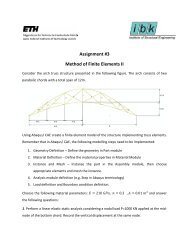
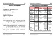
The first two analysis types, although significantly simplified, can lead to valuable conclusions
concerning the behavior of the structure and the possible collapse mechanism. The applied procedure
can be described in brief as follows. In the case of 2-D analysis the structure is assumed to consist of a
finite number of nodes interconnected by a finite number of elements. The types of elements have
been It may described expensive in section 3. toIn calculate the case of the 3-D tangent analysis the stiffness structure matrix. is assumed Into the consist of the
aforementioned Modified Newton-Raphson 2-D frames, assuming a rigid iteration diaphragm scheme assemblage it is of only their calculated horizontal dof’s in the per floor
slab. Loads may be applied at the nodes or along the elements. In both cases though, they are
transformed beginning to nodal of each loads. new load step
Modified Newton (Raphson)Method
Figure 5. Modified Newton Raphson Method
In the quasi-Newton iteration schemes the secant stiffness matrix is used
instead of the tangent matrix
After the formation of the stiffness matrix the equilibrium equations are solved by an efficient
algorithm based on the Gaussian elimination method. The structure stiffness is stored in a banded form
Institute of Structural Engineering Method of Finite Elements II 28

Simple Bar Example - Revisited
t t () i t+Δ t t+Δt ( i− 1) t+Δt ( i−1)
( Ka + Kb) Δ u = R−( Fa − Fb
)
t+Δ t () i t+Δt ( i−1) () i
with initial conditions
u = u;
F = F F = F
t+Δ t (0) t t+Δ t (0) t t+Δt (0) t
a a b b
t
u = u +Δu
t
t
CA t CA
Ka
= ; Kb
=
L L
a
if section is elastic
t ⎧=
E
C ⎨
⎩= ET
if section is plastic
b
Institute of Structural Engineering Method of Finite Elements II 29

Simple Bar Example - Revisited
Load step 1: t = 1:
( K + K ) Δ u = R− F − F
0 0 (1) 1 1 (0) 1 (0)
a b a b
⇓
2×
10
Δ u = = 6.6667×
10
7 1 1
10 ( + )
10 5
Iteration 1: ( i = 1)
4
(1) −3
u = u +Δ u = 6.6667×
10
1 (1) 1 (0) (1) −3
1 (1)
1 (1) −4
εa
= = ×
La
1 (1)
b
u
b
6.6667 10 < ε (elastic section!)
1 (1)
u
−3
ε = = 1.3333×
10 < εY
(elastic section!)
L
F
= 6.6667× 10 ; F = 1.3333×
10
1 (1) 3 1 (1) 4
a
b
0 0 (2) 1 1 (1) 1 (1)
( Ka Kb) u R Fa Fb
0
Y
Convergence in one iteration!
1 −3
+ Δ = − − = u = 6.6667×
`10
Institute of Structural Engineering Method of Finite Elements II 30

Simple Bar Example - Revisited
Load step 2: t = 2 :
( K + K ) Δ u = R− F − F
1 1 (1) 2 2 (0) 2 (0)
a b a b
⇓
(4× 10 ) − (6.6667× 10 ) − (1.333×
10 )
Δ u = = 6.6667×
10
7 1 1
10 ( + )
10 5
Iteration 1: ( i = 1)
4 3 4
(1) −3
u = u +Δ u = 1.3333×
10
2 (1) 2 (0) (1) −2
ε = 1.3333×
10 < ε (elastic section!)
2 (1) −3
a
ε
2 (1) −3
b
Y
= 2.6667×
10 > ε (plastic section!)
Y
F = 1.3333× 10 ; F = ( E ( ε − ε ) + σ ) A= 2.0067×
10
1 (1) 4 1 (1) T 2 (1) 4
a b b Y Y
( K + K ) Δ u = R− F − F ⇒Δ u = 2.2×
10
1 1 (2) 2 2 (1) 2 (1) (2) −3
a b a b
Institute of Structural Engineering Method of Finite Elements II 31

Simple Bar Example - Revisited
The procedure is repeated and the results of successive iterations are
tabulated in the accompanying table.
Institute of Structural Engineering Method of Finite Elements II 32