Solution of Equilibrium Equations in Static Analysis: LDLT Solution ...

Solution of Equilibrium Equations
in Static Analysis: LDL T Solution
15-Jun-07
Method of Finite Elements I
1

Contents
• Gauss elimination
i i
• Physical interpretation of Gauss elimination in the
context of finite element problems
• The LDL T ‐solution:
• Introduction to the procedure
• Algorithm used in computational implementations
• Efficiency
• Error considerations
• Related methods
15-Jun-07
Method of Finite Elements I
2

Review ‐ Matrices
• Positive‐definiteness: v T Av > 0 for all vectors v (semi‐
positive definite: v T Av ≥ 0 )
⎡1
2 0 0 0 0 0
⎢
• Bandwidth of a matrix A:
⎢
⎢
3 4 5 0 0 0 0
6 7 8 9 0 0 0
• p ⎥ ⎥⎥⎥⎤
1 + p 2 + 1, where a ij = 0 for j > i + p 2 or i > j + p ⎢
1 0 1 2 3 4 0 0
• Skyline of a matrix A:
• for j, j = 1,...,n: m j = i’ with a ij = 0for i < i’
m T = [1 1 2 3 4 5 6]
• Column heights of a matrix: h i = i ‐ m i for i = 1,...,n
h T = [0 1 1 1 1 1 1]
(maximum column height ht = half‐bandwidth m K )
⎢
⎢0
0 5 6 7 8 0
⎢
⎢0
0 0 9 1 2 3
⎢
⎥ ⎥⎥⎥⎥⎥ ⎣0
0 0 0 4 5 6⎦
p 1 =2, p 2 =1
15-Jun-07
Method of Finite Elements I
3

Gauss elimination
Carl F. Gauss, ca. 1850, solution of linear
systems of equations
In general:
Solve Ax=b for x
where A is a matrix of coefficients,
x is the vector of unknowns,
b is the right‐hand side vector
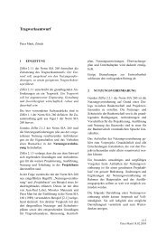
simply supported
beam with 4 transl. dofs
R 2
U 1 U 2 U 3 U 4
15-Jun-07
In the context of finite element problems:
Solve KU=R for U
where K is the stiffness matrix,
U is the displacement vector,
R is the load vector K U R
Method of Finite Elements I
4

Gauss elimination
In a Gauss elimination, we reduce the matrix of coefficients to an upper
triangular form, by a successive addition of multiples of the i th row
(i= 1,…,n –1) to the remaining n – irows j (j = i+ 1,…,n).
r2 = r2 + 4/5 r1;
r3 = r3 + (‐1/5) r1;
r4 = r4;
r3 = r3 + 16/14 r2;
r4 = r4 + (‐5/14) r2;
r4 = r4 + 20/15 r3;
15-Jun-07
Method of Finite Elements I
5

Gauss elimination
The result is an upper‐triangular matrix which we can solve for the
unknowns U i in the order U n ,UU
n‐1 ,…,UU
1 .
5 -4 1 0
0 14/5 -16/5 1
0 0 15/7 -20/7
0 0 0 5/6
U 1
U 2
U 3
U 4
0
1
8/7
7/6
• After step i (i.e. after the full addition procedure involving multiples
l
of row i), the lower right (n‐i) x (n‐i) submatrix is symmetric →
storage implications
• Solution based on non‐vanishing ihi i th diagonal element of coefficient
i
matrix in step i.
• The operations on the coefficient matrix are independent of the right‐
hand side vector.
• Any desirable order of eliminations may be chosen.
15-Jun-07
Method of Finite Elements I
6

Physical Interpretation
A physical interpretation of the operations performed in a Gauss elimination:
5 -4 1 0
6 -4 1
symmetric
6 -4
U 1
U 2
U 3
U 4
0
0
0
5 0
First equation: 5 U 1 –4 U 2 + U 3 = 0 ⇔ U 1 = 4/5 U 2 –1/5 U 3
Elimination i of U 1 from equations 2, 3 and 4 yields ild the lower right 3 x 3 submatrix
which we get after the first step of the Gauss elimination of the original matrix:
14/5 -16/5 1
-16/5 29/5 -4
1 -4 5
U 2
0
Stiffness matrix corresponding to
U 3
0 beam after release of dof 1.
U 4 0 ( dof 1“statically condensed out”)
….. 5/6 is stiffness matrix of beam after release of dofs 1, 2 and 3 (cf.
Gauss elimination: final upper triangular matrix).
15-Jun-07
Method of Finite Elements I
7

Physical Interpretation
15-Jun-07
Method of Finite Elements I
8

Physical Interpretation
15-Jun-07
Method of Finite Elements I
9

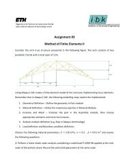
Physical Interpretation
•We get a total of n stiffness matrices of decreasing order (n, n‐1,…, 2, 1),
each describing a set of n‐i degrees of freedom (i = 0, 1,...,n‐1) of the same
physical system.
• If R≠0, then we also establish the load vectors pertaining i to these
stiffness matrices.
•The physical picture suggests that the diagonal elements remain positive
during the Gauss elimination: Stiffness should be positive; a non‐positive
diagonal element implies an unstable structure.
Here, after release of dofs U 1 , U 2
and U 3 the last diagonal element (i.e.
the stiffness at dof U 4 ) is zero.
15-Jun-07
Method of Finite Elements I
10

LDL T Solution
The successive matrix operations during a Gauss elimination can be
cast into a general form, which h leads, likewise, i to the reduction of K
to an upper triangular form, S,
− 1 − 1 − 1
Ln− 1......
L2 L1
K =
S
where
1
L i
-1
=
.
.
.
1
-l i+1,i .
with
l
k
() i
i+
j,
i
i+ j, i
=
() i
k ii
-l i+2,i .
… .
-l n,i 1
Gauss factors for the matrix
L
...... L L K
− 1 − 1 −
1
i−1 2 1
15-Jun-07
Method of Finite Elements I
11

−1 −1 −1
n− 1......
2 1
=
LDL T Solution
L L L K S
1
.
.
.
1
Solve for K:
where L i =
K = L1L2...... Ln−
1S l i+1,i i .
l i+2,i .
… .
l n,i 1
Hence,
K = LS
1
l 21 .
l 31 l 32 .
l
with L=
L1L2...... L
n−1= 41 l 42 .
. . 1
. . .
. . .
. . .
l n1 . . . . . . l n,n-1 1
15-Jun-07
Method of Finite Elements I
12

LDL T Solution
K = LS
Now =
% where d =δ s hence =
% T
S DS and since k =k %
ij ij ij , K LDS ij ji , S=
L,
, so
K
=
LDL
T
In practice:
V
=
−1
L R
⇐ LV =
R
T
−1
−
1
( )
T
U=
L D V ⇐ DL U =
V
Example: Compute L
‐1
i , i = 1, 2, 3 , L, S, D and V from
⎡ 5 −4 1 0 ⎤
⎡0⎤
⎢
4 6 4 1
⎥
⎢
⎢
− −
1
⎥
K = ⎥ and R = ⎢ ⎥
⎢
1 −
4 6 −
4
⎥
⎢ 0
⎥
⎢
⎥
⎢ ⎥
⎣ 0 1 −4 5
0
⎦
⎣ ⎦
15-Jun-07
Method of Finite Elements I
13

L
LDL T Solution
Recall the Gauss multiplication factors – they enter into L i
‐1
, i = 1, 2, 3:
−1
1
Step 1: Step 2:
r3 = r3 + 8/7 r2;
r4 = r4 + (‐5/14) r2;
r2 = r2 + 4/5 r1;
r3 = r3 + (‐1/5) r1;
r4 = r4;
Step 3:
r4 = r4 + 4/3 r3;
⎡ 1
⎤
⎡1
⎤
⎡1
⎤
⎢
4/5 1
⎥ ⎢
⎢
⎥ 1
0 1
⎥ ⎢
−
= ⎢
⎥
1
0 1
⎥
−
L
⎢ −1/5
0 1 ⎥
2
= L
⎢ 0 8/7 1 ⎥
3
= ⎢
⎥
⎢ 0 0 1 ⎥
⎢
⎥
⎢
⎥
⎢
⎥
⎣ 0 0 0 1
⎦ ⎣
0 − 5/
14
0 1
⎦
⎣
0 0 4/
3
1
⎦
(i.e. the i th column of L i
‐1
contains the multipliers of the i th step)
15-Jun-07
L
⎡ 1
⎤
⎢
4/5 1
⎥
⎢
−
⎥
1/5 −
8/7 1
⎢
⎥
⎣ 0 5/14 −4/3 1⎦
= L1L2L3
= ⎢
⎥
Method of Finite Elements I
14

LDL T Solution
Recall the pivots in the Gauss elimination – they enter into S (i.e. reduced K):
S
⎡5 −4 1 0 ⎤
⎢
14 / 5 −16 / 5 1
⎥
= ⎢
⎥
⎢
15/7 −
20/7
⎥
⎢
⎥
⎣
5/6 ⎦
First row of K
Second row of K after step 1
Third row of K after step 2
Fourth row of K after step 3
For the matrix D: d ij =δδ ij s ij
⎡5
⎤
⎢
14 / 5
⎥
D
= ⎢
⎥
⎢ 15 / 7
⎥
⎢
⎥
⎣
5/6⎦
V is the right‐hand ha side after the reduction of K to upper tia triangular form
V =
[ 0 1 8/7 7/6]
T
15-Jun-07
Method of Finite Elements I
15

Practical issues (1)
LDL T Solution
• Simultaneous computation of V and L ‐1
i .
• L and V not computed from scratch, but by modifications of K
and R.
• K is symmetric, banded and dpositive‐definite; ite the two oformer
properties permit the compact storage in a 1‐D Array,
complemented by a 1‐D address array:
K
⎡ 5 −4 1 0 ⎤
⎢
−
−
⎥
4 6 4 1
= ⎢
⎥
⎢ 1 − 4 6 − 4 ⎥
⎢
⎥
⎣ 0 1 −4 5 ⎦
a = [ 5 6 − 4 6 − 4 1 5 − 4 1]
non‐zero elements of upper half and diagonal
b = [1 2 4 7]
array indices of the diagonal elements in a
15-Jun-07
Method of Finite Elements I
16

LDL T Solution
Algorithm:
• Columnwise calculation l of l ij and d jj for j = 2,...,n, starting ti with d 11 = k 11 :
g
m , j
= km
, j
g
ij
j
j
i
∑
∑ −1 = kij
−
lrigrj
i = m +1,...,
j −1
r=
m
m
j
where m = skyline of K, m m = max{m i , m j }
now: decomposition of K to the factors D and L (or: L T )
g
ij
l
ij
= i = m
j
+1,...,
j −1
dii
d
jj
=
k
jj
−
∑
j−1
r=
m
j
l
rj
g
rj
Here: l ij denotes
an element of L T
15-Jun-07
Method of Finite Elements I
17

Algorithm:
LDL T Solution
T
−1 −
1
• compute U via V: = ( )
V
i
=
R
i
−
i
∑ − 1
r=
m
i
l
ri
V
r
U L D V
now backsubstitution: first, compute
Starting with V 1 = R 1 , compute V i for i = 2,…,n
V =
D
−1
V
Get
(n)
U
n
= V n
and
then get (successively) for U i‐1 (i = n,...,2)
V = V −l U r = m ,...,ii
−
1
( i −1) ( i)
Vr Vr lri U
i
i
= ( i−1)
U
i− 1
V i −1
in the (n ‐ i + 1) th evaluation, i.e. in the evaluation of U i‐1
18
15-Jun-07
Method of Finite Elements I
18

LDL T Solution
Practical issues (2)
• The sums over the products l rj g rj and l ri g rj do not involve terms outside the
skyline (“skyline reduction method”, “column reduction method”, “active
column solution”)
• Storage: K as compact 1‐D array
• l ij replaces g ij
• d jj replaces k jj
a = [ 5 6 − 4 6 − 4 1 5 − 4 1]
b = [1 2 4 7]
a = [ d d l d l l d l ] 24
11 22 12 33 23 13 44 34
l
• V i replaces R i
c = [ R 1
R 2
R 3
R
4]
( j)
• V k
replaces V k
(
c = [ V
1
j)
V
( j)
2
V
( j)
3
V
( j)
4
]
15-Jun-07
Method of Finite Elements I
19

LDL T Solution
Practical issues (3)
• Effective, because of skyline reduction, but the sums over the products
l rj g rj and l ri g rj can still involve zero terms. “Sparse solvers” skip the
vanishing terms.
• Ati Active column solutions: re‐order the equations to reduce column hiht heights
• Sparse solvers: re‐order the equations to eliminate operations on
elements equal to zero
15-Jun-07
Method of Finite Elements I
20

LDL T Solution
Example:
K
First, get D and L T :
d 11 = 2; now loop over all j, j = 2,…,5
j= 2: g 12 = k 12 = ‐2 g
m , j
= km
, j
l 12 = g 12 /d 11 = ‐2/2 = ‐1
d 22 = k 22 ‐ l 12 g 12 = 3 –(‐1)(‐2) = 1
⎡ 2 −2 −1⎤
⎢
3 2 0
⎥
⎢
−
⎥
= ⎢
5 −3 0 ⎥
⎢
⎥
⎢symm. 10 4
⎥
⎢
⎣
10⎥
⎦
j
j
g
ij
l
ij
= i = m
j
+ 1,...,
j − 1
d
ii
d
jj
=
k
jj
−
j
− 1
∑
lrj
r=
m
j
g
rj
⎡1⎤
⎢ 1
⎥
⎢ ⎥
→ m = ⎢2⎥
⎢ ⎥
⎢3
⎥
⎢
⎣1⎥
⎦
⎡2
−1 −1⎤
⎢
1 2 0
⎥
⎢
−
⎥
K
= ⎢
5 −
3 0
⎥
⎢
⎥
⎢
10 4 ⎥
⎢
⎣
10⎥
⎦
15-Jun-07
Method of Finite Elements I
21

LDL T Solution
j= 3: g 23 = k 23 = ‐2
l 23 = g 23 /d 22 = ‐2/1 = ‐2
g
m
,
j
= km
,
j
j j ,
d 33 = k 33 – l 23 g 23 = 5 –(‐2)(‐2) = 1
ii
⎡2 −1 −1⎤
⎢
1 2 0
⎥
⎢
−
⎥
i = m
j
+ 1,...,
j − K = ⎢ 1 −3 0 ⎥
⎢
⎥
10 4
j
∑ − 1
⎢
⎥
d
jj
= k
jj
− lrj
grj
⎢
10⎥
r=
m j
⎣
⎦
g
ij
l
ij
= 1
d
j= 4: g 34 = k 34 = ‐3
l 34 = g 34 /d 33 = ‐3/1 = ‐3
g
m , j
= km
, j
d 44 = k 44 – l 34 g 34 = 10 – (‐3)(‐3) = 1
j
j
g
ij
l
ij
= i = m
j
+ 1,...,
j − 1
d
ii
d
jj
= k
jj
−
j
− 1
∑l
rj
r=m
j
⎡2 −1 −1⎤
⎢
1 −2 0
⎥
⎢
⎥
K = ⎢ 1 −3
0 ⎥
⎢ ⎥
⎢
1 4 ⎥
g rj
⎢
⎣
10
⎥
⎦
15-Jun-07
Method of Finite Elements I
22

LDL T Solution
j= 5: g 15 = k 15 = ‐1
g 25 = k 25 – l 12 g 15 = 0 –(‐1)(‐1) = ‐1
g 2 g 35 = k 35 – l 23 g 25 = 0 – (‐2)(‐1) = ‐2
m j , j
= k
g 45 = k 45 – l 34 g 35 = 4 –(‐3)(‐2) = ‐2
g
m , j
j
l 15 = g 15 /d 11 = ‐1/2
l 25 = g 25 /d 22 = ‐1/1 = ‐11
l 35 = g 35 /d 33 = ‐2/1 = ‐2
l 45 = g 45 /d 44 = ‐2/1 = ‐2
g
ij
l
ij
= i = m
j
+ 1,...,
j − 1
d
ii
d
jj
= k
jj
−
j
∑ − 1
lrj
r=
m
j
g
rj
d 55 = k 55 – l 15 g 15 – l 25 g 25 – l 35 g 35 – l 45 g 45 = 10 – (‐1/2)(‐1) 1) – (‐1)(‐1) – (‐2)(‐2) – (‐2)(‐2) = 1/2
K
⎡
2 −
1 −
1/2
⎤
⎢
1 2 −1
⎥
⎢
−
⎥
= ⎢ 1 −3
−2
⎥
⎢
⎥
⎢
1 −
2 ⎥
⎢
⎣
1/2 ⎥
⎦
15-Jun-07
Method of Finite Elements I
23

LDL T Solution
Now, get the solution U of KU=R with R=[0 1 0 0 0] T
V 1 = R 1 = 0
i
V 2 = R 2 – l 12 V 1 = 1 –0 = 1
∑ − 1
Vi
= Ri
− l
r=
mi
V 3 = R 3 – l 23 V 2 = 0 –(‐2)(1) = 2
V 4 = R 4 – l 34 V 3 = 0 –(‐3)(2) = 6
V 5 = R 5 – l 15 V 1 – l 25 V 2 – l 35 V 3 – l 45 V 4 = 0 – 0 – (‐1)(1) – (‐2)(2) – (‐2) (6) = 17
ri
V
r
forward
reduction
Hence: V=[0 1 2 6 17] T and
V
− 1
= D V =
[0 1 2 6 34] T
V
(5) =
i = 5
V
→ U = =
5
V5 34
V V l U
V2 = V2 − l25U5 = 1 −( − 1)(34) = 35
(4) (5)
V3 = V3 − l35U5 = 2 −( − 2)(34) = 70
(4) (5)
V 4
= V 4
− l 45U
5
= 6 −( − 2)(34) = 74
U
(4) (5)
1
=
1 −
15 5 = 0 − ( − 1/ 2)(34) =
17
(4) (5)
(4)
4
V4 74
backsubstitution
b i
V = V − l U
r
( i−1) ( i)
r r ri i
= m ,..., i − 1
= = R = [ 17 35 292 70 74 4]
i
3 T
15-Jun-07
Method of Finite Elements I
24

LDL T Solution
V = V − l U r = m ,..., i − 1
( i−1) ( i)
r r ri i
i
i = 4
V = V − l U = − − =
U
(3) (4)
3 3 34 4
70 ( 3)(74) 292
(3)
3
= V3 = 292
R = [17 35 292 74 34] T
i = 3 V2 = V2 − l23U3 = −( − )( ) =
(2) (3)
2 2 23 3
35 ( 2)(292) 619
(2)
2
= V2 = 619
U
R =
[17 619 292 74 34] T
i = 2
V = V − l U = − − =
U = = R = U = [ 636 619 292 74 34]
T
(1) (2)
1 1 12 2
17 ( 1)(619) 636
(1)
1
V1 636
15-Jun-07
Method of Finite Elements I
25

Efficiency of the solution
•form K = i – m i , for all i > m K (i.e. for constant column height): LDL T
decomposition requires n[m K + (m K ‐1)+ … +1] = ½ nm K2 operations,
reduction and backsubstitution of a load vector requires 2nm K operations
•in general (without constant column height): for decomposition of K and
reductionand backsubstitutionof R we get total of ½ Σ(i –m i ) 2 + 2 Σ(i –m i )
operations
• number of operations is governed by the pattern of nonzero elements in
thematrix ti
15-Jun-07
Method of Finite Elements I
26

Error Estimate
•Now we use t=3 digits for Gauss algorithm:
Note hats (matrices represented with t=3) and bars (approximate
solution – t=3) over unknown displacements
15-Jun-07
Method of Finite Elements I
27

Error Estimate
• Truncation errors (we solve equations exactly):
• Round‐off errors:
• Total errors:
15-Jun-07
Method of Finite Elements I
28

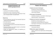
Error Estimate
Bathe, page 749: Summary on truncation and roundoff
errors in solving KU = R
15-Jun-07
Method of Finite Elements I
29

Related Methods
•Cholesky factorization
• Static ti condensation
• Substructure analysis
• Frontal solution
15-Jun-07
Method of Finite Elements I
30