Numerical Modeling of Fluid Flow in Porous Media and in Driven ...
Numerical Modeling of Fluid Flow in Porous Media and in Driven ...
Numerical Modeling of Fluid Flow in Porous Media and in Driven ...

Create successful ePaper yourself
Turn your PDF publications into a flip-book with our unique Google optimized e-Paper software.
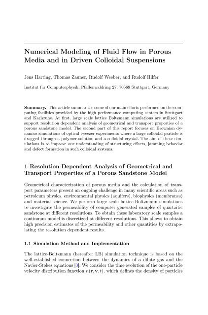
<strong>Numerical</strong> <strong>Model<strong>in</strong>g</strong> <strong>of</strong> <strong>Fluid</strong> <strong>Flow</strong> <strong>in</strong> <strong>Porous</strong><br />
<strong>Media</strong> <strong>and</strong> <strong>in</strong> <strong>Driven</strong> Colloidal Suspensions<br />
Jens Hart<strong>in</strong>g, Thomas Zauner, Rudolf Weeber, <strong>and</strong> Rudolf Hilfer<br />
Institut für Computerphysik, Pfaffenwaldr<strong>in</strong>g 27, 70569 Stuttgart, Germany<br />
Summary. This article summarizes some <strong>of</strong> our ma<strong>in</strong> efforts performed on the comput<strong>in</strong>g<br />
facilities provided by the high performance comput<strong>in</strong>g centers <strong>in</strong> Stuttgart<br />
<strong>and</strong> Karlsruhe. At first, large scale lattice Boltzmann simulations are utilized to<br />
support resolution dependent analysis <strong>of</strong> geometrical <strong>and</strong> transport properties <strong>of</strong> a<br />
porous s<strong>and</strong>stone model. The second part <strong>of</strong> this report focuses on Brownian dynamics<br />
simulations <strong>of</strong> optical tweezer experiments where a large colloidal particle is<br />
dragged through a polymer solution <strong>and</strong> a colloidal crystal. The aim <strong>of</strong> these simulations<br />
is to improve our underst<strong>and</strong><strong>in</strong>g <strong>of</strong> structur<strong>in</strong>g effects, jamm<strong>in</strong>g behavior<br />
<strong>and</strong> defect formation <strong>in</strong> such colloidal systems.<br />
1 Resolution Dependent Analysis <strong>of</strong> Geometrical <strong>and</strong><br />
Transport Properties <strong>of</strong> a <strong>Porous</strong> S<strong>and</strong>stone Model<br />
Geometrical characterization <strong>of</strong> porous media <strong>and</strong> the calculation <strong>of</strong> transport<br />
parameters present an ongo<strong>in</strong>g challenge <strong>in</strong> many scientific areas such as<br />
petroleum physics, environmental physics (aquifers), biophysics (membranes)<br />
<strong>and</strong> material science. We perform large scale lattice-Boltzmann simulations<br />
to <strong>in</strong>vestigate the permeability <strong>of</strong> computer generated samples <strong>of</strong> quartzitic<br />
s<strong>and</strong>stone at different resolutions. To obta<strong>in</strong> these laboratory scale samples a<br />
cont<strong>in</strong>uum model is discretized at different resolutions. This allows to obta<strong>in</strong><br />
high precision estimates <strong>of</strong> the permeability <strong>and</strong> other quantities by extrapolat<strong>in</strong>g<br />
the resolution dependent results.<br />
1.1 Simulation Method <strong>and</strong> Implementation<br />
The lattice-Boltzmann (hereafter LB) simulation technique is based on the<br />
well-established connection between the dynamics <strong>of</strong> a dilute gas <strong>and</strong> the<br />
Navier-Stokes equations [3]. We consider the time evolution <strong>of</strong> the one-particle<br />
velocity distribution function n(r, v,t), which def<strong>in</strong>es the density <strong>of</strong> particles
350 J. Hart<strong>in</strong>g et al.<br />
with velocity v around the space-time po<strong>in</strong>t (r,t). By <strong>in</strong>troduc<strong>in</strong>g the assumption<br />
<strong>of</strong> molecular chaos, i.e. that successive b<strong>in</strong>ary collisions <strong>in</strong> a dilute gas are<br />
uncorrelated, Boltzmann was able to derive the <strong>in</strong>tegro-differential equation<br />
for n named after him [3]<br />
( ) dn<br />
∂ t n + v ·∇n = , (1)<br />
dt<br />
coll<br />
where the right h<strong>and</strong> side describes the change <strong>in</strong> n due to collisions.<br />
The LB technique arose from the realization that only a small set <strong>of</strong> discrete<br />
velocities is necessary to simulate the Navier-Stokes equations [4]. Much<br />
<strong>of</strong> the k<strong>in</strong>etic theory <strong>of</strong> dilute gases can be rewritten <strong>in</strong> a discretized version.<br />
The time evolution <strong>of</strong> the distribution functions n is described by a discrete<br />
analogue <strong>of</strong> the Boltzmann equation [10]:<br />
n i (r + c i Δt, t + Δt) =n i (r,t)+Δ i (r,t) , (2)<br />
where Δ i is a multi-particle collision term. Here, n i (r,t) gives the density<br />
<strong>of</strong> particles with velocity c i at (r,t). In our simulations, we use 19 different<br />
discrete velocities c i . The hydrodynamic fields, mass density ϱ <strong>and</strong> momentum<br />
density j = ϱu are moments <strong>of</strong> this velocity distribution:<br />
ϱ = ∑ i<br />
n i ,<br />
j = ϱu = ∑ i<br />
n i c i . (3)<br />
We use a l<strong>in</strong>ear collision operator,<br />
Δ i = − 1 τ (n i − n eq<br />
i ) , (4)<br />
where we assume that the local particle distribution relaxes to an equilibrium<br />
state n eq<br />
i at a s<strong>in</strong>gle rate τ [1]. By employ<strong>in</strong>g the Chapman-Enskog expansion<br />
[3, 4] it can be shown that the equilibrium distribution<br />
[<br />
n eq<br />
i = ϱω ci 1+3c i · u + 9 2 (c i · u) 2 − 3 ]<br />
2 u2 , (5)<br />
with the coefficients ω ci<br />
c i = |c i |,<br />
correspond<strong>in</strong>g to the three different absolute values<br />
ω 0 = 1 3 , ω1 = 1 18 , ω√2 = 1<br />
36 , (6)<br />
<strong>and</strong> the k<strong>in</strong>ematic viscosity<br />
ν = η = 2τ − 1 ,<br />
ϱ f 6<br />
(7)<br />
properly recovers the Navier-Stokes equations
<strong>Flow</strong> <strong>in</strong> <strong>Porous</strong> <strong>Media</strong> <strong>and</strong> <strong>Driven</strong> Colloidal Suspensions 351<br />
∂u<br />
∂t +(u∇)u = − 1 ϱ ∇p + η Δu , ∇u =0. (8)<br />
ϱ<br />
We use LB3D [6], a highly scalable parallel LB code, to implement the<br />
model. LB3D is written <strong>in</strong> Fortran 90 <strong>and</strong> designed to run on distributedmemory<br />
parallel computers, us<strong>in</strong>g MPI for communication. It can h<strong>and</strong>le up<br />
to three different fluid species <strong>and</strong> is able to model flow <strong>in</strong> complex geometries<br />
as it occurs for example <strong>in</strong> porous media. In each simulation, the fluid is<br />
discretized onto a cubic lattice, each lattice po<strong>in</strong>t conta<strong>in</strong><strong>in</strong>g <strong>in</strong>formation about<br />
the fluid <strong>in</strong> the correspond<strong>in</strong>g region <strong>of</strong> space. Each lattice site requires about<br />
a kilobyte <strong>of</strong> memory per lattice site so that, for example, a simulation on a<br />
128 3 lattice would require around 2.2GB <strong>of</strong> memory. The code runs at over<br />
6 · 10 5 lattice site updates per second per CPU on a recent mach<strong>in</strong>e, <strong>and</strong> has<br />
been observed to have roughly l<strong>in</strong>ear scal<strong>in</strong>g up to order 3·10 3 compute nodes<br />
(see below).<br />
Simulations on larger scales have not been possible so far due to the lack <strong>of</strong><br />
access to a mach<strong>in</strong>e with a higher processor count. The largest simulation we<br />
performed used a 1536 3 lattice <strong>and</strong> ran on the AMD Opteron based cluster <strong>in</strong><br />
Karlsruhe. There, it is not possible to use a larger lattice s<strong>in</strong>ce the amount <strong>of</strong><br />
memory per CPU is limited to 4GB <strong>and</strong> only 1024 processes are allowed with<strong>in</strong><br />
a s<strong>in</strong>gle job. On the NEC SX-8 <strong>in</strong> Stuttgart, typical system sizes are <strong>of</strong> the<br />
order <strong>of</strong> 256×256×512 lattice sites. The output from a simulation usually takes<br />
the form <strong>of</strong> a s<strong>in</strong>gle float<strong>in</strong>g-po<strong>in</strong>t number for each lattice site, represent<strong>in</strong>g, for<br />
example, the density <strong>of</strong> a fluid at that site. Therefore, a density field snapshot<br />
from a 128 3 system would produce output files <strong>of</strong> around 8MB.<br />
Writ<strong>in</strong>g data to disk is one <strong>of</strong> the bottlenecks <strong>in</strong> large scale simulations. If<br />
one simulates a 1024 3 system, each data file is 4GB <strong>in</strong> size. The situation gets<br />
even more critical when it comes to the files needed to restart a simulation.<br />
Then, the state <strong>of</strong> the full simulation lattice has to be written to disk requir<strong>in</strong>g<br />
0.5TB <strong>of</strong> disk space. LB3D is able to benefit from the parallel file systems<br />
available on many large mach<strong>in</strong>es today, by us<strong>in</strong>g the MPI-IO based parallel<br />
HDF5 data format [7]. Our code is very robust regard<strong>in</strong>g different platforms or<br />
cluster <strong>in</strong>terconnects: even with moderate <strong>in</strong>ter-node b<strong>and</strong>widths it achieves<br />
almost l<strong>in</strong>ear scal<strong>in</strong>g for large processor counts with the only limitation be<strong>in</strong>g<br />
the available memory per node. The platforms on which our code has been<br />
successfully used <strong>in</strong>clude various supercomputers like the NEC SX-8, IBM<br />
pSeries, SGI Altix <strong>and</strong> Orig<strong>in</strong>, Cray T3E, Compaq Alpha clusters, as well as<br />
low cost 32- <strong>and</strong> 64-bit L<strong>in</strong>ux clusters.<br />
Dur<strong>in</strong>g the last year, a substantial effort has been <strong>in</strong>vested to improve<br />
the performance <strong>of</strong> LB3D <strong>and</strong> to optimize it for the simulation <strong>of</strong> flow <strong>in</strong><br />
porous media. Already dur<strong>in</strong>g the previous report<strong>in</strong>g period, we improved the<br />
performance on the SX8 <strong>in</strong> Stuttgart substantially by rearrang<strong>in</strong>g parts <strong>of</strong> the<br />
code <strong>and</strong> by try<strong>in</strong>g to <strong>in</strong>crease the length <strong>of</strong> the loops. These changes were<br />
proposed by the HLRS support staff. However, while the code scales very well<br />
with the number <strong>of</strong> processors used, the s<strong>in</strong>gle CPU performance is still below
352 J. Hart<strong>in</strong>g et al.<br />
what one could expect from a lattice Boltzmann implementation on a vector<br />
mach<strong>in</strong>e. The vector operation ratio is about 93%, but due to the <strong>in</strong>herent<br />
structure <strong>of</strong> our multiphase implementation, the average loop length is only<br />
between 20 <strong>and</strong> 30. Thus, the performance <strong>of</strong> our code stays below 1GFlop/s.<br />
For this reason, we are currently perform<strong>in</strong>g most <strong>of</strong> our simulations on the<br />
Opteron cluster XC2 <strong>in</strong> Karlsruhe. Our code performs extremely well there<br />
<strong>and</strong> shows almost l<strong>in</strong>ear scal<strong>in</strong>g to up to 1024 CPU’s. Further, due to extensive<br />
improvements <strong>of</strong> the code dur<strong>in</strong>g the last year, we were able to <strong>in</strong>crease the<br />
per CPU performance by a factor <strong>of</strong> about two.<br />
The lattice Boltzmann code can read voxel based 3D representations <strong>of</strong><br />
porous media. Such data can either be obta<strong>in</strong>ed from XMT measurements <strong>of</strong><br />
real samples or from numerical models. In order to compute the permeability<br />
<strong>of</strong> such a sample, the velocity field v(x) <strong>and</strong> pressure field p(x) as created by<br />
the LB simulations are required. For a liquid with dynamic viscosity η, the<br />
permeability κ is def<strong>in</strong>ed accord<strong>in</strong>g to Darcy’s law<br />
〈v(x)〉 x∈S = − κ η 〈∇p〉 x∈S (9)<br />
<strong>and</strong> thus<br />
κ = −η 〈v(x)〉 x∈S<br />
, (10)<br />
〈∇p〉 x∈S<br />
with 〈v(x)〉 x∈S be<strong>in</strong>g the velocity component <strong>in</strong> flow direction averaged over<br />
the full pore space S. We approximate the average pressure gradient 〈∇p〉 x∈S<br />
<strong>of</strong> the full sample like<br />
〈∇p〉 x∈S ≈ 〈p(x)〉 x∈OUT −〈p(x)〉 x∈IN<br />
, (11)<br />
aL<br />
with IN/OUT represent<strong>in</strong>g the plane, perpendicular to the flow direction, <strong>in</strong><br />
front <strong>of</strong> / beh<strong>in</strong>d the porous medium, the total length L (<strong>in</strong> voxel) <strong>and</strong> a the<br />
resolution. The accelerat<strong>in</strong>g force, <strong>in</strong> positive z-direction, is applied as a body<br />
force only <strong>in</strong> the first quarter <strong>of</strong> the “IN-flow” buffer before the sample, another<br />
buffed “OUT-flow” was added after the sample. Periodic boundary conditions<br />
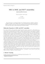
<strong>in</strong> flow direction are be<strong>in</strong>g imposed. Fig. 1 shows the simulation setup for a<br />
sample with resolution a =10μm <strong>and</strong> voxel dimension 136x136x168 <strong>and</strong> the<br />
two “IN/OUT-flow” buffers.<br />
1.2 Sample Creation <strong>and</strong> Simulation Setup<br />
Because appropriately sized digital samples at sufficient resolutions are not<br />
available from experimental data, a cont<strong>in</strong>uum model <strong>of</strong> a quartzitic s<strong>and</strong>stone<br />
was discretized at different resolutions <strong>and</strong> sizes (Table 1) <strong>and</strong>then<br />
thresholded to generate digital voxel data. For details expla<strong>in</strong><strong>in</strong>g the model<br />
see [2]. With <strong>in</strong>creas<strong>in</strong>g resolution a the microstructure becomes more <strong>and</strong><br />
more resolved at the expense <strong>of</strong> <strong>in</strong>creas<strong>in</strong>g the amount <strong>of</strong> data <strong>and</strong> CPU time
<strong>Flow</strong> <strong>in</strong> <strong>Porous</strong> <strong>Media</strong> <strong>and</strong> <strong>Driven</strong> Colloidal Suspensions 353<br />
Fig. 1. <strong>Porous</strong> medium with pore space (blue) <strong>and</strong> the two IN/OUT-flow buffers<br />
shown. The flow is <strong>in</strong> positive z-direction, the sample size is 136x136x168 voxel, at<br />
aresolution<strong>of</strong>a =10μm<br />
<strong>in</strong> simulations. To f<strong>in</strong>d a good compromise between a high enough resolution<br />
<strong>and</strong> manageable systems for LB-simulations, geometrical characterizations for<br />
each <strong>of</strong> our samples were calculated (See Fig. 3,4).<br />
Table 1. List <strong>of</strong> available digitized samples<br />
Sidelength<br />
[voxel]<br />
Resolution<br />
a[μm]<br />
Number <strong>of</strong><br />
samples<br />
256 80 1<br />
256 40 1<br />
512/256 20 1/8<br />
512/256 10 8/16<br />
512/256 5 8/16<br />
512/256 2.5 8/16<br />
Typical lattice-Boltzmann simulation required 50,000–80,000 simulation<br />
steps to reach stationary flow with<strong>in</strong> the pore space. Simulations were performed<br />
on 64 to 512 CPU’s. For the total <strong>of</strong> 83 samples (<strong>in</strong>clud<strong>in</strong>g calibration<br />
test runs) more than 80,000 CPU hours were required. The LB3D code scales<br />
l<strong>in</strong>early <strong>and</strong> memory usage was moderate, mak<strong>in</strong>g <strong>in</strong>vestigations <strong>of</strong> larger samples<br />
feasible <strong>and</strong> tempt<strong>in</strong>g. Fig. 2 shows the average time for one simulation<br />
step <strong>and</strong> per voxel <strong>in</strong> nano seconds (left axis). The average time was calculated<br />
from more than 100 runs on different systems with vary<strong>in</strong>g parameters <strong>and</strong>
354 J. Hart<strong>in</strong>g et al.<br />
sizes. The speedup factor is def<strong>in</strong>ed as<br />
speedup(n) = (total runtime on 4 CPU′ s)<br />
(total runtime on n CP U ′ s)<br />
The total runtime <strong>of</strong> a simulation is the time the program needs for it’s full<br />
execution. The speedup factor was def<strong>in</strong>ed with reference to a run on 4 CPU’s<br />
because on 4-core systems one physical node has 4 CPU’s. The communication<br />
<strong>and</strong> I/O overhead for a simulation run on one physical node is negligible,<br />
compared to network communications.<br />
Fig. 2. LB3D code scal<strong>in</strong>g behavior. The sequential lattice Boltzmann code is known<br />
to scale l<strong>in</strong>early with the sample size (voxel). The time per simulation step <strong>and</strong> per<br />
voxel is shown on the left axis. The speedup, shown on the right axis<br />
1.3 Geometric Properties at Different Resolutions<br />
For each sample geometrical properties such as the porosity, specific surface<br />
<strong>and</strong> mean/total curvature have been calculated to <strong>in</strong>vestigate their behavior<br />
with chang<strong>in</strong>g resolution <strong>and</strong> subsampl<strong>in</strong>g. From the resolution dependent<br />
porosity φ(a) (Fig. 3) conclusions can be drawn which resolution ranges approximate<br />
the true physical porosity well enough <strong>and</strong> thus, are suitable for<br />
simulations. Increas<strong>in</strong>g the resolution (lower a) beyond a certa<strong>in</strong> po<strong>in</strong>t (here<br />
approx. a =5− 10μm) will not justify the <strong>in</strong>crease <strong>in</strong> data <strong>and</strong> CPU time but<br />
on the other h<strong>and</strong> low resolutions (a =50− 80μm) will most likely not yield<br />
relevant simulation data, because not even the sample porosity is close to the<br />
true porosity <strong>of</strong> the physical s<strong>and</strong>stone. As can be seen <strong>in</strong> (Fig. 3), subsamples<br />
much smaller than 256μm will not represent the full sample well. The data
<strong>Flow</strong> <strong>in</strong> <strong>Porous</strong> <strong>Media</strong> <strong>and</strong> <strong>Driven</strong> Colloidal Suspensions 355<br />
Fig. 3. Porosity φ for the full sample <strong>and</strong> subsamples at different resolutions a.<br />
The data for the full sample is extrapolated to the true physical porosity at a=0.<br />
With <strong>in</strong>creas<strong>in</strong>g resolution the porosity approaches the true physical porosity. Large<br />
enough subsamples, 512μm <strong>and</strong> 256μm, approximate the full sample (size 1024μm)<br />
porosity well. Subsamples at 128μm are not representative for the full sample<br />
for the full sample (black l<strong>in</strong>e) can be extrapolated to approximate the true<br />
physical porosity as a → 0.<br />
Local porosity distributions [8, 9] are def<strong>in</strong>ed as<br />
μ(φ, L, a) = 1 ∑<br />
δ(φ − φ(x, L, a))<br />
m<br />
x∈S<br />
where φ(x, L, a) is the local porosity <strong>of</strong> a measurement cell with sidelength L<br />
at the position x <strong>and</strong> a sample resolutions a. S is the full sample, m is the<br />
number <strong>of</strong> evaluated measurement cells <strong>and</strong> δ is the Dirac delta function.<br />
To calculate this local porosity distribution a small cubic measurement<br />
cell, with sidelength L, is be<strong>in</strong>g moved through the whole sample <strong>and</strong> at all<br />
positions x, thelocalporosityφ(x, L, a) with<strong>in</strong> the cell is calculated.<br />
The local porosity distributions μ(φ, L, a), asshown<strong>in</strong>Fig.4, givethe<br />
probability density that a r<strong>and</strong>omly placed measurement cell with sidelength<br />
L has a porosity φ whenthesampleresolutionisa. In our case they have<br />
a maximum close to the porosity <strong>of</strong> the full sample at that resolution. For<br />
resolutions a =40, 20, 10μm the distributions are well converged. Together<br />
with other geometric properties def<strong>in</strong>ed with<strong>in</strong> Local porosity theory μ(φ, L, a)<br />
can be used to estimate the permeability [8].<br />
The lattice Boltzmann simulations calculated the velocity field <strong>and</strong> pressure<br />
field for all available samples with different resolutions. In Fig. 5 the<br />
z-Component v z , component <strong>in</strong> flow direction, <strong>of</strong> the velocity field for a sample<br />
with resolution a =10μm <strong>and</strong> voxel size 136x136x168 is shown. The pore<br />
structure <strong>of</strong> the same sample is shown <strong>in</strong> Fig. 1. The “IN-flow” buffer, where<br />
the liquid is accelerated to a speed <strong>of</strong> approx 0.002 lattice units, is shown <strong>in</strong>
356 J. Hart<strong>in</strong>g et al.<br />
Fig. 4. Local porosity distributions for a measurement cell size L = 320μm at<br />
different resolutions a. Very high resolutions (a = 5μm) yield bad statistics, at<br />
the size <strong>of</strong> the measurement cell used here. The distributions for resolutions a =<br />
40, 20, 10μm are very similar <strong>in</strong> shape, the mean porosity changes accord<strong>in</strong>g to Fig. 3<br />
green at the top. All voxel with v z > 0 are shown <strong>in</strong> translucent blue. The<br />
brown isosurfaces depict areas where v z > 0.001 <strong>in</strong> lattice units, be<strong>in</strong>g half <strong>of</strong><br />
the maximum speed <strong>in</strong> the “IN-flow” buffer. They represent channels where the<br />
liquid flows fast. The flow through the porous medium is not homogeneous,<br />
even if the porous medium is quite homogeneous at this resolution.<br />
In addition to the geometric characterizations <strong>and</strong> the velocity fields high<br />
precision permeability calculations (Tbl. 2) for all 83 samples have been<br />
performed <strong>and</strong> are now been critically analyzed for accuracy, to ga<strong>in</strong> further<br />
<strong>in</strong>sight <strong>in</strong>to their resolution dependence <strong>and</strong> thereby <strong>in</strong>to the nature <strong>of</strong> fluid<br />
transport with<strong>in</strong> highly complex geometries.<br />
Table 2. Selected permeability results <strong>of</strong> the full sample (1024μm) for different resolutions.<br />
An relative error <strong>of</strong> 0.05 has been estimated, result<strong>in</strong>g from the <strong>in</strong>accuracy<br />
<strong>of</strong> the velocity field, calculated by the LB-simulation<br />
Resolution [μm] Permeability [μm 2 ]<br />
40 1.7±0.043<br />
20 2.2±0.055<br />
10 1.9±0.047
<strong>Flow</strong> <strong>in</strong> <strong>Porous</strong> <strong>Media</strong> <strong>and</strong> <strong>Driven</strong> Colloidal Suspensions 357<br />
Fig. 5. Z-Component <strong>of</strong> the velocity field. <strong>Fluid</strong> is accelerated <strong>in</strong> the IN-flow<br />
buffer on top(green). Shown <strong>in</strong> translucent blue is the complete volume fraction with<br />
v z > 0. Darker regions correspond to smaller velocities. All areas with a velocity<br />
with v z > 0.001 are shown as isosurfaces. Channels with large connected isosurfaces<br />
thus carry the ma<strong>in</strong> flow through the porous medium<br />
2 Simulation <strong>of</strong> Optical Tweezer Experiments<br />
A colloidal suspension is a mixture <strong>of</strong> a fluid <strong>and</strong> particles or droplets with a<br />
length scale <strong>of</strong> some nanometers to micrometers suspended <strong>in</strong> it. Colloids are<br />
a common part <strong>of</strong> everyday life. Substances like pa<strong>in</strong>t, glue, milk, blood <strong>and</strong><br />
fog are just some examples. Due to their technical applications, colloids are<br />
studied <strong>in</strong> several discipl<strong>in</strong>es, among them physics, chemistry, <strong>and</strong> eng<strong>in</strong>eer<strong>in</strong>g.<br />
Colloidal particles are too large to be affected directly by quantum mechanical<br />
effects. On the other h<strong>and</strong>, they are still small enough to be affected<br />
by thermal fluctuations. Therefore, colloidal suspensions are an <strong>in</strong>terest<strong>in</strong>g<br />
system to study thermodynamic phenomena like diffusion, phase transitions<br />
<strong>and</strong> more rare phenomena like stochastic resonance <strong>and</strong> critical Casimir forces.<br />
In solid state physics, colloidal crystals are used as model systems to study<br />
defect formation, crystal structures <strong>and</strong> melt<strong>in</strong>g. In contrast to many systems<br />
<strong>in</strong> these fields, which are on the nanometer scale, colloidal suspensions can<br />
be observed <strong>and</strong> manipulated directly us<strong>in</strong>g techniques like video microscopy,<br />
confocal microscopy, total <strong>in</strong>ternal reflection microscopy (TIRM) <strong>and</strong> optical<br />
tweezers. This <strong>of</strong>fers numerous possibilities to control these systems on a per<br />
particle basis.
358 J. Hart<strong>in</strong>g et al.<br />
We study dynamical properties <strong>of</strong> colloidal suspensions us<strong>in</strong>g computer<br />
simulations. The advantage <strong>of</strong> simulations is that parameters can be controlled<br />
<strong>in</strong> ways that are not accessible <strong>in</strong> experiments. Also, <strong>in</strong> many cases,<br />
<strong>in</strong>formation is available that cannot be measured directly <strong>in</strong> a real system.<br />
Over the past decades, several simulation techniques have become available,<br />
which model different aspects <strong>of</strong> suspensions.<br />
Methods like molecular dynamics <strong>and</strong> Brownian dynamics only model the<br />
dynamics <strong>of</strong> the suspended colloidal particles <strong>and</strong> h<strong>and</strong>le the solvent implicitly<br />
by add<strong>in</strong>g simplified forces to mimic the solvents behavior. Other approaches<br />
like lattice-Boltzmann models, dissipative particle dynamics <strong>and</strong> stochastic<br />
rotation dynamics simulate the complete fluid <strong>and</strong> couple it to suspended<br />
particles. While the first set <strong>of</strong> methods are computationally very efficient,<br />
more complicated hydrodynamic effects are usually not taken <strong>in</strong>to account<br />
(polarization <strong>of</strong> the solvent). The methods that do simulate the full fluid field<br />
can reproduce hydrodynamic effects, but achiev<strong>in</strong>g quantitative accuracy far<br />
from equilibrium is still a challenge. Here, we focus on the Brownian dynamics<br />
technique <strong>in</strong> order to be able to simulate very large systems with an affordable<br />
amount <strong>of</strong> CPU time.<br />
The dynamics <strong>of</strong> driven suspensions can be exam<strong>in</strong>ed by dragg<strong>in</strong>g a colloidal<br />
particle through it. In this article we present our simulations <strong>of</strong> a particle<br />
dragged through a colloidal crystal <strong>and</strong> a suspension <strong>of</strong> coiled polymers us<strong>in</strong>g<br />
an optical tweezer. The focus <strong>of</strong> the optical tweezer is moved with time,<br />
thereby pull<strong>in</strong>g the impurity along.<br />
Optical tweezers trap a colloid (or even an atom) <strong>in</strong> the focus <strong>of</strong> a laser<br />
beam: this is because a dielectric is always driven along the field gradient.<br />
They are a very important tool <strong>in</strong> s<strong>of</strong>t condensed matter physics: colloids can<br />
not only be trapped, they can also be moved around <strong>in</strong>dividually by mov<strong>in</strong>g<br />
the focus <strong>of</strong> the laser beam. Thereby the colloidal system can be controlled<br />
with an accuracy that would be impossible for an atomic system. The optical<br />
tweezer is modeled with a harmonic potential, i.e. as if the impurity were<br />
connected with the trap center by an ideal spr<strong>in</strong>g.<br />
The simulations are motivated by experiments performed by R. Dullens<br />
<strong>in</strong> the group <strong>of</strong> C. Bech<strong>in</strong>ger <strong>in</strong> Stuttgart <strong>and</strong> C. Gutsche <strong>in</strong> the group <strong>of</strong><br />
F. Kremer <strong>in</strong> Leipzig, respectively. In both cases, the simulation parameters<br />
are chosen to reproduce the experimental conditions as closely as possible.<br />
2.1 Simulation Setup<br />
The experiments are simulated us<strong>in</strong>g a modified Brownian dynamics (BD)<br />
method which <strong>in</strong>cludes some <strong>of</strong> the hydrodynamics caused by the dragged<br />
colloid, as expla<strong>in</strong>ed <strong>in</strong> Ref. [11]. The colloids/polymers <strong>and</strong> the probe particle<br />
are modeled as hard spheres with their respective radii.<br />
We use a rectangular simulation volume with periodic boundary conditions<br />
<strong>in</strong> all three directions. Due to long range hydrodynamic <strong>in</strong>teractions, large
<strong>Flow</strong> <strong>in</strong> <strong>Porous</strong> <strong>Media</strong> <strong>and</strong> <strong>Driven</strong> Colloidal Suspensions 359<br />
systems are required <strong>in</strong> order to reduce f<strong>in</strong>ite size effects. Thus, we typically<br />
h<strong>and</strong>le several hundred thous<strong>and</strong> particles <strong>in</strong> a s<strong>in</strong>gle simulation.<br />
The probe particle is trapped <strong>in</strong> a mov<strong>in</strong>g parabolic potential V (r) =<br />
1<br />
2 ar2 , mimick<strong>in</strong>g the optical tweezer. In the case <strong>of</strong> the polymer suspension,<br />
the potential has a spr<strong>in</strong>g constant <strong>of</strong> a =7.5 × 10 −5 pN/nm, which gives a<br />
better signal to noise ratio than the experimental value <strong>of</strong> 8.5 × 10 −2 pN/nm.<br />
Figure 6 shows a cut out <strong>of</strong> a snapshot <strong>of</strong> our simulation setup used to describe<br />
the experiments performed by the group <strong>in</strong> Leipzig.<br />
Fig. 6. A cut through the simulated system, where a probe particle is dragged<br />
through a suspension (from [5]). The arrow <strong>in</strong>dicates the direction <strong>of</strong> motion <strong>of</strong> the<br />
probe particle<br />
In conventional BD, the two most important aspects <strong>of</strong> hydrodynamics<br />
felt by the suspended particles are taken <strong>in</strong>to account, namely the Stokes<br />
friction <strong>and</strong> the Brownian motion. Correspond<strong>in</strong>gly, this is done by add<strong>in</strong>g to<br />
a molecular dynamics simulation two additional forces. The Langev<strong>in</strong> equation<br />
describes the motion a Brownian particle with radius R at position r(t) as<br />
m ¨r(t) =6πηRṙ(t)+F r<strong>and</strong> (t)+F ext (r,t), (12)<br />
where the first term models the Stokes friction <strong>in</strong> a solvent <strong>of</strong> viscosity η,<br />
F ext (r,t) is the sum <strong>of</strong> all external forces like gravity, forces exerted by other<br />
suspended particles, <strong>and</strong>, for the colloid, the optical trap. F r<strong>and</strong> (t) describes<br />
the thermal noise which gives rise to the Brownian motion. The r<strong>and</strong>om force<br />
on different particles is assumed to be uncorrelated, as well as the force on<br />
the same particle at different times. It is further assumed to be Gaussian with<br />
zero mean. The mean square deviation <strong>of</strong> the Gaussian (i.e., the amplitude <strong>of</strong><br />
the correlator) is given by the fluctuation-dissipation theorem as<br />
〈|F r<strong>and</strong> | 2 〉 =12πηRk B T. (13)<br />
This conventional BD scheme is widely used to simulate suspensions because<br />
it is well understood, not difficult to implement, <strong>and</strong> needs much less computational<br />
resources than a full simulation <strong>of</strong> the fluid. However, this simulation<br />
method does not resolve hydrodynamic <strong>in</strong>teractions between particles. In<br />
particular, the long-ranged hydrodynamic <strong>in</strong>teractions between the dragged
360 J. Hart<strong>in</strong>g et al.<br />
colloid <strong>and</strong> the surround<strong>in</strong>g particles are not modeled. However, <strong>in</strong> the system<br />
we consider, these <strong>in</strong>teractions are important, as the dragged colloid moves<br />
quickly <strong>and</strong> has a strong <strong>in</strong>fluence on the flow field around it. Therefore, the<br />
BD scheme is modified such that the effect caused by the flow field around<br />
the dragged colloid is <strong>in</strong>cluded. This is achieved by calculat<strong>in</strong>g the friction<br />
force on the small particles with radius R c not with respect to a rest<strong>in</strong>g fluid<br />
(F =6πηR c u), but with respect to the flow field caused by the mov<strong>in</strong>g colloid.<br />
The friction force then is<br />
F =6πηR c (u − v(r)), (14)<br />
where v(r) is the flow field around the mov<strong>in</strong>g colloid at a position r with<br />
respect to the colloid’s center. This correction leads to the <strong>in</strong>clusion <strong>of</strong> two<br />
hydrodynamics-mediated effects. Due to the large component <strong>of</strong> the flow field<br />
along the direction <strong>of</strong> motion, both, <strong>in</strong> front <strong>and</strong> beh<strong>in</strong>d the probe, small<br />
colloids are dragged along. Also the flow <strong>of</strong> particles is advected around the<br />
mov<strong>in</strong>g probe particle, i.e., obstacles are moved out <strong>of</strong> the way to its sides.<br />
Both these effects lead to a reduction <strong>of</strong> drag force on the driven colloid.<br />
2.2 Investigat<strong>in</strong>g the Stiffness <strong>and</strong> Occurrence <strong>of</strong> Defects <strong>in</strong><br />
Colloidal Crystals<br />
To analyze the effects <strong>of</strong> the disturbance due to the dragged probe particle, we<br />
can either measure the distance that the probe stays beh<strong>in</strong>d the focus <strong>of</strong> the<br />
optical tweezer - <strong>and</strong> thereby the force required to drag the impurity through<br />
the crystal - or exam<strong>in</strong>e the reaction <strong>of</strong> the crystal itself. With our simulations<br />
we show that <strong>in</strong> a colloidal crystal, the velocity-force relation for the dragged<br />
colloidal particle is close to l<strong>in</strong>ear despite the complicated surround<strong>in</strong>g. It is<br />
also shown that the <strong>in</strong>ter-colloid potential does have an <strong>in</strong>fluence on the drag<br />
force, though not as strong as velocity. This is one example <strong>of</strong> a result that<br />
could not be obta<strong>in</strong>ed easily <strong>in</strong> experiments. Us<strong>in</strong>g maps <strong>of</strong> average particle<br />
density <strong>and</strong> defect distributions, we illustrate the effect <strong>of</strong> the dragged colloidal<br />
particle on the crystal structure.<br />
An example <strong>of</strong> a rather small system is given <strong>in</strong> Fig. 7. For large tweezer<br />
velocities, much larger crystals are needed <strong>and</strong> for study<strong>in</strong>g the relaxation <strong>of</strong><br />
the crystal, we also have to simulate for at least a 100 to 300 seconds <strong>of</strong> real<br />
time caus<strong>in</strong>g these simulations to cost up to a few thous<strong>and</strong> CPU hours each.<br />
2.3 Dragg<strong>in</strong>g a Colloidal Probe Through a Polymer Suspension<br />
The second system we consider is a suspension <strong>of</strong> coiled polymers which are<br />
modeled as hard spheres. A colloidal particle is dragged through the suspension<br />
at high velocities. In the experiment <strong>and</strong> <strong>in</strong> the simulation, a drag force is<br />
measured that is higher than that calculated from the suspension’s viscosity as<br />
obta<strong>in</strong>ed from a shear rheometer. This <strong>in</strong>crease <strong>in</strong> drag force can be expla<strong>in</strong>ed
<strong>Flow</strong> <strong>in</strong> <strong>Porous</strong> <strong>Media</strong> <strong>and</strong> <strong>Driven</strong> Colloidal Suspensions 361<br />
Fig. 7. Simulation <strong>of</strong> a large colloidal particle dragged through a crystal consist<strong>in</strong>g<br />
<strong>of</strong> smaller colloids by means <strong>of</strong> an optical tweezer. The color<strong>in</strong>g denotes defects<br />
occurr<strong>in</strong>g due to the distortion <strong>of</strong> the crystal<br />
by a jamm<strong>in</strong>g <strong>of</strong> polymers <strong>in</strong> front <strong>of</strong> the mov<strong>in</strong>g colloidal particle. In contrast<br />
to experiments, this jamm<strong>in</strong>g can be observed directly <strong>in</strong> computer simulations<br />
as the positions <strong>of</strong> the polymers are available. The simulation results<br />
are compared to dynamic density functional theory calculations by Rauscher<br />
et. al <strong>and</strong> experimental results by Gutsche et al.. A very good quantitative<br />
agreement between experiment, theory <strong>and</strong> simulation is observed [5].<br />
From the simulation data, it is possible to measure the effective polymer<br />
concentration around the dragged colloid. To accomplish this, we take about<br />
2000 two dimensional slices <strong>of</strong> the simulation <strong>and</strong> move each snapshot such<br />
that the position <strong>of</strong> the colloid co<strong>in</strong>cides <strong>in</strong> each snapshot. We calculate the<br />
probability for each <strong>of</strong> the 200 × 200 b<strong>in</strong>s to be occupied by a polymer by<br />
averag<strong>in</strong>g over all snapshots. Polymers accumulate <strong>in</strong> front <strong>of</strong> the colloidal<br />
particle <strong>and</strong> the concentration <strong>in</strong> the back is reduced due to the f<strong>in</strong>ite Peclet<br />
number <strong>of</strong> the polymers. For high polymer concentrations, the probability to<br />
f<strong>in</strong>d a polymer <strong>in</strong> front <strong>of</strong> the colloid is close to one. The region right beh<strong>in</strong>d<br />
the colloid is almost clear <strong>of</strong> polymers, because the polymers get advected<br />
away from the colloid before they can diffuse <strong>in</strong>to this region.<br />
Our model reproduces very well the experimentally found l<strong>in</strong>ear relation<br />
between drag force <strong>and</strong> the drag velocity for different polymer concentrations.<br />
As higher drag velocities require a larger system (even with periodic boundary<br />
conditions) <strong>and</strong> short numerical time steps, we are limited to about 80 μm/s<br />
by the available computational resources <strong>and</strong> time. However, the l<strong>in</strong>earity <strong>of</strong><br />
the drag force with respect to the velocity at high enough velocities allows to<br />
extrapolate to the higher velocities used <strong>in</strong> the experiments.
362 J. Hart<strong>in</strong>g et al.<br />
Fig. 8. Polymer density around the colloidal particle averaged over 2000 snapshots<br />
<strong>of</strong> the system. Lighter colors correspond to higher polymer densities. Also visible are<br />
density oscillations <strong>in</strong> front <strong>of</strong> the colloid, which are characteristic for hard sphere<br />
systems<br />
3 Conclusion<br />
In this report we have presented results from lattice Boltzmann simulations<br />
<strong>of</strong> fluid flow <strong>in</strong> porous media <strong>and</strong> the simulation <strong>of</strong> optical tweezer experiments.<br />
In particular the AMD Opteron cluster <strong>in</strong> Karlsruhe has been found<br />
to perform particularly well with our simulation codes. In the case <strong>of</strong> porous<br />
media simulations we have demonstrated that we are able to systematically<br />
determ<strong>in</strong>e the permeability <strong>of</strong> digitized quartzitic s<strong>and</strong>stone samples – even if<br />
the resolution <strong>of</strong> the samples is very high result<strong>in</strong>g <strong>in</strong> the need <strong>of</strong> substantial<br />
computational resources.<br />
In the second part <strong>of</strong> this article we reported on our Brownian dynamics<br />
simulations <strong>of</strong> optical tweezer experiments, where a large probe particle is<br />
trapped by a laser beam <strong>and</strong> dragged either through a colloidal crystal or<br />
through a polymer suspension. In both cases, quantitative agreement with<br />
experimental data was observed.<br />
Acknowledgments<br />
We are grateful to the High Performance Comput<strong>in</strong>g Center <strong>in</strong> Stuttgart<br />
<strong>and</strong> the Scientific Supercomput<strong>in</strong>g Center <strong>in</strong> Karlsruhe for provid<strong>in</strong>g access<br />
to their NEC SX-8 <strong>and</strong> HP 4000 mach<strong>in</strong>es. We would like to thank Bibhu<br />
Biswal, Peter Diez, <strong>and</strong> Frank Raischel for fruitful discussions. This work was<br />
supported by the collaborative research center 716 <strong>and</strong> the DFG program<br />
“nano- <strong>and</strong> micr<strong>of</strong>luidics”.<br />
References<br />
1. P.L. Bhatnagar, E.P. Gross, <strong>and</strong> M. Krook. Model for collision processes <strong>in</strong> gases.<br />
I. small amplitude processes <strong>in</strong> charged <strong>and</strong> neutral one-component systems.<br />
Phys. Rev., 94(3):511, 1954.
<strong>Flow</strong> <strong>in</strong> <strong>Porous</strong> <strong>Media</strong> <strong>and</strong> <strong>Driven</strong> Colloidal Suspensions 363<br />
2. B. Biswal, P.E. Oren, R. Held, S. Bakke, <strong>and</strong> R. Hilfer. Stochastic multiscale<br />
model for carbonate rocks. Phys.Rev. E, 75:061303, 2007.<br />
3. S. Chapman <strong>and</strong> T.G. Cowl<strong>in</strong>g. The mathematical theory <strong>of</strong> non-uniform gases.<br />
Cambridge University Press, second edition, 1952.<br />
4. U. Frisch, D. d’Humiéres, B. Hasslacher, P. Lallem<strong>and</strong>, Y. Pomeau, <strong>and</strong> J.P.<br />
Rivet. Lattice gas hydrodynamics <strong>in</strong> two <strong>and</strong> three dimensions. Complex Systems,<br />
1(4):649, 1987.<br />
5. C. Gutsche, F. Kremer, M. Krüger, M. Rauscher, J. Hart<strong>in</strong>g, <strong>and</strong> R. Weeber.<br />
Colloids dragged through a polymer solution: experiment, theory <strong>and</strong> simulation.<br />
Submitted for publication, arXiv:0709.4142, 2007.<br />
6. J. Hart<strong>in</strong>g, M. Harvey, J. Ch<strong>in</strong>, M. Venturoli, <strong>and</strong> P.V. Coveney. Large-scale<br />
lattice Boltzmann simulations <strong>of</strong> complex fluids: advances through the advent<br />
<strong>of</strong> computational grids. Phil.Trans.R.Soc.Lond.A, 363:1895–1915, 2005.<br />
7. 2003. HDF5 – a general purpose library <strong>and</strong> file format for stor<strong>in</strong>g scientific<br />
data, http://hdf.ncsa.uiuc.edu/HDF5.<br />
8. R. Hilfer. Transport <strong>and</strong> relaxation phenomena <strong>in</strong> porous media. Adv. Chem.<br />
Phys., XCII:299, 1996.<br />
9. R. Hilfer. Local porosity theory <strong>and</strong> stochastic reconstruction for porous media.<br />
In K. Mecke <strong>and</strong> D. Stoyan, editors, Statistical Physics <strong>and</strong> Spatial Statistics,<br />
volume 554 <strong>of</strong> Lecture Notes <strong>in</strong> Physics, page 203, Berl<strong>in</strong>, 2000. Spr<strong>in</strong>ger.<br />
10. A.J.C. Ladd <strong>and</strong> R. Verberg. Lattice-boltzmann simulations <strong>of</strong> particle-fluid<br />
suspensions. J. Stat. Phys., 104(5):1191, 2001.<br />
11. M. Rauscher, M. Krüger, A. Dom<strong>in</strong>guez, <strong>and</strong> F. Penna. A dynamic density<br />
functional theory for particles <strong>in</strong> a flow<strong>in</strong>g solvent. J. Chem. Phys., 127:244906,<br />
2007.