Molecular dynamics and Monte Carlo simulation methods for soft ...

Molecular dynamics
and Monte Carlo
simulation methods
for soft matter
Martin Vögele
17. 04. 2012
Contents
1 Soft Matter 2
1.1 What is soft matter? . . . . . . . . . . . . . . . . . . . . . . . . . . . . . . . 2
1.2 Why is soft matter soft? . . . . . . . . . . . . . . . . . . . . . . . . . . . . . 2
1.3 Types of soft matter . . . . . . . . . . . . . . . . . . . . . . . . . . . . . . . 3
1.3.1 Colloids . . . . . . . . . . . . . . . . . . . . . . . . . . . . . . . . . . 3
1.3.2 Amphiphiles . . . . . . . . . . . . . . . . . . . . . . . . . . . . . . . . 3
1.3.3 Polymeres . . . . . . . . . . . . . . . . . . . . . . . . . . . . . . . . . 4
2 Molecular Dynamics Simulation 5
2.1 Principles . . . . . . . . . . . . . . . . . . . . . . . . . . . . . . . . . . . . . 5
2.2 Algorithms . . . . . . . . . . . . . . . . . . . . . . . . . . . . . . . . . . . . 5
2.3 Observables . . . . . . . . . . . . . . . . . . . . . . . . . . . . . . . . . . . . 6
2.4 Applications . . . . . . . . . . . . . . . . . . . . . . . . . . . . . . . . . . . . 6
3 Monte Carlo Simulation 7
3.1 Basics . . . . . . . . . . . . . . . . . . . . . . . . . . . . . . . . . . . . . . . 7
3.2 Applications . . . . . . . . . . . . . . . . . . . . . . . . . . . . . . . . . . . . 7
3.3 MC Integration . . . . . . . . . . . . . . . . . . . . . . . . . . . . . . . . . . 7
3.3.1 Calculating π . . . . . . . . . . . . . . . . . . . . . . . . . . . . . . . 7
3.3.2 Importance Sampling . . . . . . . . . . . . . . . . . . . . . . . . . . . 7
3.4 Metropolis Algorithm . . . . . . . . . . . . . . . . . . . . . . . . . . . . . . 8
4 Boundary Conditions 9
4.1 Types of Boundary Conditions . . . . . . . . . . . . . . . . . . . . . . . . . 9
4.2 Minimum Image Convention . . . . . . . . . . . . . . . . . . . . . . . . . . . 9
4.3 Linked Cells and Neighbor Lists . . . . . . . . . . . . . . . . . . . . . . . . . 9

1 Soft Matter
1.1 What is soft matter?
The classical sorts of matter usually cosidered in physics are all homogeneous already on
scales of nanomters. If one looks at a crystalline solid or at some kind of liquid, there is
no more structure visible on that scale. But there are also more complex materials, where
there are still structures up to nanometers which determine their typical behavior. This
is shown for as suspension in figure 1, where we can see the different length scales with
different structures: First the atomic scale, then the scale of the single layers and at last
the range where the interface is only a line and just the different areas of oil and water are
visible.
Figure 1: lenght scales of soft matter [4]
Based on this, we will use the following definition.
Soft matter:
Systems, whose properties are determined by structures in the mesoscopic scale (range
between nano- and micrometers).
1.2 Why is soft matter soft?
Figure 2: shearing [4]
The term soft matter describes one of its most important properties. We can understand
this by estimating the shear modulus µ which as the resistance against a shearing force

(see figure 2). It is defined by
F
L x L y
= µ ∆L x
L z
.
As we can seee, the dimension is E · L −3 . For soft matter, the energy normally is in
the thermical range, a typical value is k B T = (1/40) eV. The decisive part is the lattice
constant. Let us assume a colloidal crystal. Its lattice size is 10000 times the one of a
normal crystal, because that is the order of the determining structures. This means that
soft matter has a shear modulus which is about 10 12 times smaller than the one of a typical
solid.
1.3 Types of soft matter
1.3.1 Colloids
Colloids are particles or drops with a size between 1 nm and 1 µm inside a liquid. The
size differences are just in that range, where the surrounding liquid can be approximated
as a continuum. This surrounding liquid causes thermal movement of the colloids by small
collisions. The resulting movement of the particles is well-known as Brownian motion.
The particles themselves can interact by hard sphere repulsion, electrostatic forces, Van
der Waals forces and by entropic effects. Most of these interactions can easily be modified:
the electrostatic force by inserting salt whose ions shield the electric potential, the Van
der Waals forces by changing the refraction index of the medium and the hard shpere and
entropic effects by changing the form of the particles.
Important for applications is the nonlinear dynamic behavior when a force is exerted. this
is for example used in dispersion paint, which becomes hard as soon as it isn’t pressed
against the wall any more.
Figure 3: colloids in a medium [1]
1.3.2 Amphiphiles
Amphiphiles are molecules that are made up of a hydrophile head and lipophile tail. That
is why they preferrably accumulate at interfaces when put into a system containing water
and oil. Substances that are made up of these components are called microemulsions and
one can roughly distinguish between three sorts:

• more water ⇒ drops of oil in water
• more oil ⇒ drops of water in oil
• equal amounts ⇒ bicontinuous phase: water-oil-network
In case there is only water and amphiphiles, they form either spherical aggregates (mycels)
or double layers (membranes).
The widest-known application are tensides used for cleaning. A simulation for such a
tenside is shown in figure 4.
Figure 4: MD simulation of a system with 3350 tenside and 3200 water molecules.
bottom right: random start configuration. [6]
1.3.3 Polymeres
Polymeres are chains of monomeres, that are connected by covalent bonds. These bonds
can be rotated or flipped, which results in many degrees of freedom. This is why for
long polymeres the conformation entropy is the dominat term in the free energy. So their
behaivior can be described very well statistical methods, for example as a random walk.
Figure 5: typical conformation of a fluctuating polymer chain, simulated with MC
method [4]

2 Molecular Dynamics Simulation
2.1 Principles
In molecular dynamics simulations, one assumes a material (solid, liquid or gas) to contain a
certain number N of classical particles. These particles interact by (mostly semiempirical)
potentials v ij = v(⃗r ij ). By differentiating these potentials, one obtains the forces
⃗f i = ∑ i≠j
⃗f ij = − ∑ i≠j
∂v(⃗r ij )
∂⃗r i
which can be used to solve Newton’s equations for each particle.
m i¨⃗ri = ⃗ f i
So the trajectories for all particles can be obtained and used for calculating macroscopic
properties.
2.2 Algorithms
As all many body problems, MD equations can’t be solved analytically. That’s why numerical
algorithms have to be used. A good algorithm must be exact but nevertheless fast,
so one has to find compromises. It also needs to be time-reversible and certain properties
must be conserved (energy, momentum,...).
The most most common algorithms for MD are:
• Runge-Kutta 4th order
• Verlet algorithm
• Velocity Verlet algorithm
• Predictor-corrector method
Here the Verlet algorithm shall be shown as an example. It is derived by using two Taylor
series of ⃗r i (backward and forward):
⃗r i (t + ∆t) = ⃗r i (t) + ∆t · ˙⃗r i + (∆t)2 ¨⃗r i + (∆t)3 d 3 ⃗r i
2 6
⃗r i (t − ∆t) = ⃗r i (t) − ∆t · ˙⃗r i + (∆t)2 ¨⃗r i − (∆t)3
2 6
Add both equations and use ¨⃗r i = ⃗ f i
m i
:
dt 3 + O(∆t4 )
d 3 ⃗r i
dt 3 + O(∆t4 )
⃗r i (t + ∆t) = 2⃗r i (t) − ⃗r i (t − ∆t) + ⃗ f i
m i
∆t 2 + O(∆t 4 )
In this algorithm, the velocity is not needed, but the local coordinates of two steps before.
The velocity can though be calculated as:
v(t) = ⃗r i(t + ∆t) − ⃗r i (t − ∆t)
2∆t
Because of using forward and backward series the Verlet algorithm is time-reversible and
it can also be shown that the energy is conserved.

2.3 Observables
The MD simulation at first only gives the trajectories of the particles, but they can hardly
be compared with experiments and anyway we are mostly interested in the macroscopic
behavior. So macroscopic values, called observables, must be determined. they are usually
evaluated by statistical averages over all particles. That’s where we need the ergodic hpothesis,
which says that in a chaotic system, all accessible microstates are equally probable
over a long time, so that the time average is equal to the statistical average: Ā t = 〈A〉.
Important observables are the mean potential energy per particle, the mean kinetic energy
per particle respectively the temperature or pressure.
2.4 Applications
• Nobel gases (classical example: liquid Argon)
• Solid state physics:
all sorts of solids, especially alloys
• Astrophysics:
planetary motion, behavior of galaxies
• Fluid dynamics:
Liquids that are too complex for assuming continuum
• Biochemistry:
Large molecules, proteins

3 Monte Carlo Simulation
3.1 Basics
Monte Carlo simulations use probability theory to solve mathematical problems. the most
important principles for the stochastical models are the law of large numbers and the
central limit theorem which make shure that the probabilistic algorithm converges to a
reproducible result for a sufficient number of random experiments. The results of such
random experiments must always be analysed statistically. Depending on how elaborate
the problem is, one can use naive methods with uniformly distributed random numbers or
adapted distributions, which is called importance sampling.
3.2 Applications
• Calculating integrals, especially in higher dimensions
• evolution of galaxies
• production processes
• stock markets
• weather and climate
• calculating observables in quantum field theory
• virtual reality and artificial intelligence
3.3 MC Integration
3.3.1 Calculating π
One of the most simple (and the
best-known) example for a Monte
Carlo integration is the stochastical
determination of π. The algorithm
is quite easy: Create a
square with a quarter circle in it.
Then choose N total random points
in the square and count those who
are inside the circle. The ratio is
just π 4 .
π
4 = N inside
N total
Figure 6: statistical calculation of π [8]
3.3.2 Importance Sampling
Suppose we want to calculate averages of the type
∫
d⃗r exp [−βU(⃗r)] A(⃗r)
〈A〉 = ∫
d⃗r exp [−βU(⃗r)]

with p(⃗r) being the probability density to find the system in a state around ⃗r:
∫
exp [−βU(⃗r)]
p(⃗r) = with Z = d⃗r exp [−βU(⃗r)]
Z
Our problem is that the direct calculation of Z is too time-consuming. The solution is using
importance sampling: We generate random states according to a probability distribution
w(⃗r). So for the average holds:
〈A〉 ≈
∑ N
i=1 exp [−βU(⃗r i)] A(⃗r i )/w(⃗r i )
∑ N
i=1 exp [−βU(⃗r i)] /w(⃗r i )
If we choose w(⃗r) = exp [−βU(⃗r)] the average 〈A〉 simplifies:
⇒ 〈A〉 ≈ 1 N
N∑
A(⃗r i )
i=1
3.4 Metropolis Algorithm
The Metropolis algorithm creates a series of random variables, where the probability for a
new state only depends on the probability for the previous one (Markov chain). Starting
from the initial value x 0 , generate a potential successive value x 1 and calculate the transition
probability p(x 0 , x 1 ). Then generate a random number r ∈ [0, 1] and sccept the new
value if p(x 0 , x 1 ) > r.
Figure 7: 2D Ising model 300×300, spin up/down as white/black. [7]
One very famous example is the Ising model for magnetization, where spins are placed on a
lattice with external magnetic field H z . It is assumed that they can only be +1 or −1. The
energy of the system is determined by the Hamiltonian Ĥ = − 1 2
∑ij J ∑
ijs i s j + H z i s i.
The spins flip with a certain probability p = exp[−β(E new − E old )] for E new > E old and
p = 1 for E new < E old . In this model, critical points can be determined and domains of
different magnetization can be observed as in figure 7.

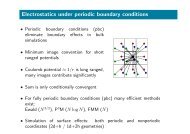
4 Boundary Conditions
4.1 Types of Boundary Conditions
The number of particles in a simulation is
limited by calculation time and memory capacity.
For sufficiently small systems, the
boundary conditions can be obtained directly
from the real problem. But most real
systems are much larger. And because usually
there is a different behavior at the surface
and inside the system, artificial boundary
conditions must be defined.
One option is the hard walls model, where
every particle hitting the wall is reflected.
These walls are like a vessel for the simulated
material. But surface and volume
can not be scaled linearly, which results in
many unwanted effects.
The more common choice are therefore periodic
bondary conditions: A particle that
Figure 8: periodic boundary conditions
leaves the simulation box, enters at the
opposite side with same velocity. This is
equivalent to an infinitely large, periodic volume, which often is much nearer to the properties
of a macroscopic system.
4.2 Minimum Image Convention
Periodic boundary conditions result in an infinite number of particles. This would lead to
an infinite number of interactions which would need infinitely much time to be calculated.
This problem is solved by the minimum image convention. For each particle, one can
consider only the region inside a so called cut-off radius r cut , where the interaction potential
is truncated. This is a very good approximation for short range interactions.
4.3 Linked Cells and Neighbor Lists
There are two ways of speeding up a calculation with beriodic boundary conditions.
The first one is the linked cell method. The simulation area is partitioned into cells and
one must consider only particles in neighbor cells. Of course, the side length of the cells
must be bigger than r cut or else the potential is cut off too near.
The second possibility is using neigbor lists, that contains for each particle all neighbors
inside a list radius r l > r cut and only those are used for the calculation. These lists must
be updated from time to time, so this method is only useful for large numbers of particles.

References
[1] SoftSimu - Biophysics and Soft Matter. http://www.softsimu.net
[2] Allen, M. P. ; Tildesley, D. J.: Computer Simulation of Liquids. Oxford University
Press, USA, 1989. – ISBN 0198556454
[3] Frenkel, Daan ; Smit, Berend: Understanding Molecular Simulation, Second Edition:
From Algorithms to Applications. Academic Press, 2002. – ISBN 0–12–267351–4
[4] Gompper, Gerhard ; Dhont, Jan K. G. ; Richter, Dieter: Komplexe Materialien
auf mesoskopischer Skala: Was ist Weiche Materie? In: Physik in unserer Zeit 34
(2003), Nr. 1, S. 12–18. – ISSN 1521–3943
[5] Griebel, Michael ; Knapek, Stephan ; Zumbusch, Gerhard ; Caglar, Attila: Numerische
Simulation in der Moleküldynamik: Numerik, Algorithmen, Parallelisierung,
Anwendungen. Springer, 2004. – ISBN 3–540–41856–3
[6] Hentschke, R. Theoretische Chemische Physik. http://constanze.materials.uniwuppertal.de/Beispiele.html
[7] Juul, Jeppe. The Ising Model. http://jeppejuul.com/proposed-projects/bachelorsproject/the-ising-model/
[8] Wikipedia: Kreiszahl — Wikipedia, Die freie Enzyklopädie.
http://de.wikipedia.org/w/index.php?title=Kreiszahl&oldid=101469010. 2012. –
[Online; Stand 8. April 2012]