Lecture Notes - Institute for Computational Physics - UniversitÃ¤t ...

Simulation Methods II 

Maria Fyta - Jens Smiatek 

Institute for Computational Physics 

Universität Stuttgart 

Apr. 11 2013

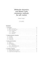
Course contents 

First principles methods 

Hartree-Fock 

Density-funtional-theory 

Møller-Plesset 

Classical Simulations 

Molecular Dynamics 

Classical force fields and water models 

Coarse-grained models 

Hydrodynamic methods 

lattice-Boltzmann 

Brownian Dynamics 

Dissipative Particle Dynamics (DPD) 

Stochastic Rotation Dynamics (SRD) 

Free energy methods 

Overview of multiscale methods 

http://www.icp.uni-stuttgart.de M.Fyta 2/25

Course where & when 

Thursdays, 11:30-13:00, ICP Seminar room 

Exceptions: 02.05 

Monday 29.4 at 08:30-10:00 instead. 

Tutorials 

New worksheets every other week handed out every 2 nd Thursday 

Discussion meetings and tutorials; Friday 08:00-10:00 – ICP CIP-Pool 

Worksheets due every 2 nd Tuesday. 

First discussion meeting (first worksheet): 19.4 

First tutorial: 26.4 

First worksheet due date: 23.4 

Exam 

Prerequisite: 50% of the total points in the tutorials 

Oral examination at the end of the semester 


Recommended Literature 

D. Frenkel and B. Smit, Understanding Molecular Simulation, Academic Press, 

San Diego, 2002. 

M.P. Allen and D.J. Tildesley, Computer Simulation of Liquids, Oxford Science 

Publications, Clarendon Press, Oxford, 1987. 

D. C. Rapaport, The Art of Molecular Dynamics Simulation, Cambridge University 

Press, 2004. 

D. P. Landau and K. Binder, A guide to Monte Carlo Simulations in Statistical 

Physics, Cambridge, 2005. 

M. E. J. Newman and G. T. Barkema, Monte Carlo Methods in Statistical Physics. 

Oxford University Press, 1999. 

J.M. Thijssen, Computational Physics, Cambridge (2007) 

S. Succi, The Lattice Boltzmann Equation for Fluid Dynamics and Beyond, Oxford 

Science Publ. (2001). 

M.E. Tuckermann, Statistical Mechanics: Theory and Moleculr Simulation, Oxford 

Graduate Texts (2010). 

M.O. Steinhauser, Computational Multiscale Modeling of Fluids and Solids, 

Springer, (2008). 

A. Leach, Molecular Modelling: Principles and Applications, Pearson Education 

Ltd. (2001). 

R.M. Martin, Electronic Stucture, Basic Theory and Practical Methods, 

Cambridge (2004). 

E. Kaxiras, Atomic and electronic structure of solids, Cambridge (2003). 


Computational Physics 

Bridge theory and experiments 

Verify or guide experiments 

Involves different spatial and temporal scales 

Extraction of a wider range of properties, mechanical, thermodynamic, 

optical, electronic, etc... 

Accuracy vs. Efficiency! 



Scales-methods-systems


Introduction to electronic structure 

Source: commons.wikimedia.org 

Different properties according to atom type and number, i.e. number of 

electrons and their spatial and electronic configurations. 


Electronic configuration 

Distribution of electrons in atoms/molecules in atomic/molecular orbitals 

Electrons described as moving independently in orbitals in an average 

field created by othe orbitals 

Electrons jump between configurations through emission/absorption of 

a photon 

Configurations are described by Slater determinants 

Source: Wikipedia 


Electronic shells 

Dual nature of electrons: particle and waves BUT “old” electronic shell 

concept helps an intuitive understanding of the (double due to spin 

up/down) allowed energy states for an electron 

Source: chemistry.beloit.edu 

Ground and excited states 

Energy associated with each electron is that of its orbital. 

Ground state: The configuration that corresponds to the lowest 

electronic energy. 

Excited state: Any other configuration.

Pauli exclusion principle 

No electron in the same atom can have the same values for all four 

quantum numbers. 

Quantum numbers 

principal quantum number n: atomic energy level (n ≥ 1) 

azimuthal(angular) quantum number l: subshell, magnitude of angular 

momentum (L 2 = 2 l(l + 1), l=0,1,2,...,n-1) 

magnetic quantum number m l : specific cloud in subshell, projection of 

orbital quantum momentum along specified axis 

(L z = m l , − l − l + 1, ..., l − 1, l) 

spin projection quantum number m s : spin, projection of spin angular 

momentum along specified axis 

(S z = m s , m s = −s, −s + 1, ...., s − 1, s) 


Periodic table of the elements 

Source: chemistry.about.com 

Example for Carbon [C] 6 electrons: ground state = 1s 2 2s 2 2p 2 


Bulk vs. finite systems - electronic structure 

Source:http://www2.warwick.ac.uk/

Bulk systems (crystalline/non-crystalline materials) 

Energy bands, band gap=(valence – conduction) band energy 

Band structure (in k-space) 

electronic density of states 

Example: Carbon, diamond and graphite 

[Dadsetani & Pourghazi, Diam. Rel. Mater., 15, 1695 (2006)]

Finite systems - (bio)molecules, clusters 

Distinct energy levels 

HOMO (highest occupied molecular orbital), LUMO (lowest unoccupied 

molecular orbial) 

band gap= (HOMO – LUMO) energy 


Example: adamantane 

[McIntosh et al, PRB, 70, 045401 (2001)] 


Finite systems - (bio)molecules, clusters 

Distinct energy levels 

HOMO (highest occupied molecular orbital), LUMO (lowest unoccupied 

molecular orbial) 

band gap= (HOMO-LUMO) energy 


Example: Adenine-Thymine base-pair in DNA 

R.L.Barnett et al, J. Mater. Sci., 42, 8894 (2007)] 


Electronic structure 

Probability distribution of electrons in chemical systems 

State of motion of electrons in an electrostatic field created by the nuclei 

Extraction of wavefunctions and associated energies through the 

Schrödinger equation: 

i ∂ ∂t Ψ = ĤΨ 

time − dependent 

EΨ = ĤΨ 

time − independent 

Solves for: 

bonding and structure 

electronic, magnetic, and optical properties of materials 

chemistry and reactions. 


Time-independent molecular Schrödinger equation 

( ˆT e + V ee + V ek + ˆT k + V kk )Ψ(r, R) = EΨ(r, R) 

r, R: electron, nucleus coordinates 

ˆT e , ˆT k : electron, nucleus kinetic energy operator 

V ee : electron-electron repulsion 

V ek : electron-nuclear attraction 

V kk : nuclear-nuclear repulsion 

E: total molecular energy 

Ψ(r, R): total molecular wavefunction 

Born-Oppenheimer approximation 

Electrons much faster than nuclei → separate nuclear from electronic 

motion 

Solve electronic and nuclear Schrödinger equation, Ψ e (r; R) and Ψ k (r) 

with Ψ = Ψ k · Ψ e . 


Approximations in electronic structure methods 

Common approximations: 

in the Hamiltonian, e.g. changing from a wavefunction-based to a 

density-based description of the electronic interaction 

simplification of the electronic interaction term 

in the description of the many-electron wavefunction 

Often the electronic wavefunction of a system is expanded in terms of 

Slater determinants, as a sum of anti-symmetric electron wavefunctions: 

∑ 

Ψ el (⃗r 1 , s 1 , ⃗r 2 , s 2 , ..., ⃗r N , s N ) = 

m 1 ,m 2 ,...,m N 

C m1 ,m 2 ,...,m N 

|φ m1 (⃗r 1 , s 1 )φ m2 (⃗r 2 , s 2 )...φ mN ( ⃗r N , s N )| 

where ⃗r i , s 1 the cartesian coordinates and the spin components. The 

components φ mN ( ⃗r N , s N ) are one-electron orbitals. 


Basis-sets 

Choices 

Bulk systems: plane waves 

Molecules/finite systems: atomic-like orbitals 

Finite basis set 

The smaller the basis, the poorer the representation, i.e. accuracy of 

results 

The larger the basis, the larger the computational load. 

Minimum basis sets: 

only atomic orbitals containing all electrons of neutral atom, e.g. for H only 

s-function, for 1 st -row of periodic table, two s-functions (1s and 2s) and one 

set of p-functions (2p x , 2p y , 2p z ). 

Improvements 

double all functions: Double Zeta (DZ) basis 

triple all functions: Triple Zeta (TZ) basis 

polarization functions (higher angular momentum functions) 

mixed basis-sets, contracted basis-sets (3-21G, 6-31G, 6-311G, ...). 


Basis-sets 

Plane-waves 

Periodic functions 

Bloch’s theorem for periodic solids: φ mN ( ⃗r N , s N ) = u n,k (⃗r)exp(i ⃗ k ·⃗r) 

Periodic u expanded in plane waves with expansion coefficients 

depending on the reciprocal lattice vectors: 

u n,k (⃗r) = 

∑ 

c nk ( G)exp(i ⃗ G ⃗ ·⃗r) 

| G|≤|G ⃗ max 

Atomic-like orbitals 

φ mN ( ⃗r N , s N ) = ∑ n D nmχ n (⃗r) 

Gaussian-type orbitals: 

χ ζ,n,l,m (r, θ, φ) = NY l,m (θ, φ)r 2n−2−l exp(−ζr 2 ) 

χ ζ,lx ,l y ,l z 

(x, y, z) = Nx lx y ly z lz exp(−ζr 2 ) 

the sum l x , l y , l z determines the orbital. 


Common aspects in electronic structure methods 

Pseudopotentials 

core electrons not considered explicitly (chemically inert); nucleus a 

classical point charge 

effects of core electrons on valence electrons are replaced by 

pseudopotentials 

electronic Schrödinger equation solved for valence electrons. 

Forces 

Electrostatic interactions are considered between nuclei and electrons 

in electronic structure methods 

Hellmann-Feynman theorem 

once spatial distribution of electrons obtained through Schrödinger 

equation, all forces of the system can be calculated using classical 

electrostatics 

∫ 

dE 

dλ = 

ψ ⋆ (λ) dĤλ 

dλ ψ(λ)dτ 


Optimization: wavefunctions and geometries 

numerical approximations of the wavefunction by successive iterations 

variational principle, convergence by minimizing the total energy: 

E ≤ 〈Φ|H|Φ〉 

geometry optimization: nuclear forces computed at the end of 

wavefunction optimization process 

nuclei shifted along direction of computed forces → new 

wavefunction(new positions) 

process until convergence: final geometry corresponds to global 

minimum of potential surface energy 

Self consistent field (SCF) 

Particles in the mean field created by the other particles 

Final field as computed from the charge density is self-consistent with 

the assumed initial field 

equations almost universally solved through an iterative method. 


ab initio methods 

Solve Schrödinger’s equation associated with the Hamiltonian of the 

system 

ab initio (first-principles): methods which use established laws of 

physics and do not include empirical or semi-empirical parameters; 

derived directly from theoretical principles, with no inclusion of 

experimental data 

Popular ab initio methods 

Hartree-Fock 

Density functional theory 

Møller-Plesset perturbation theory 

Multi-configurations self consistent field (MCSCF) 

Configuration interaction (CI), Multi-reference configuration interaction 

Coupled cluster (CC) 

Quantum Monte Carlo 

Reduced density matrix approaches

Lecture Notes - Institute for Computational Physics - UniversitÃ¤t ...

Create successful ePaper yourself

Delete template?

Save as template?