Adaptive AM–FM Signal Decomposition With Application to ... - ICS

PANTAZIS et al.: ADAPTIVE AM–FM SIGNAL DECOMPOSITION WITH APPLICATION TO SPEECH ANALYSIS 293
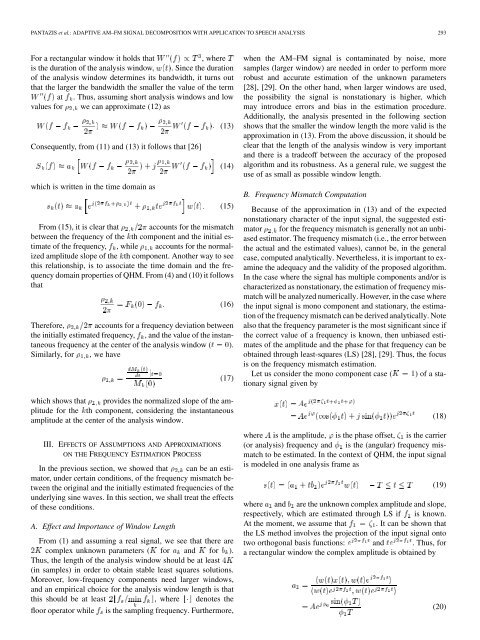
For a rectangular window it holds that
, where
is the duration of the analysis window, . Since the duration
of the analysis window determines its bandwidth, it turns out
that the larger the bandwidth the smaller the value of the term
at . Thus, assuming short analysis windows and low
values for we can approximate (12) as
Consequently, from (11) and (13) it follows that [26]
which is written in the time domain as
(13)
(14)
(15)
From (15), it is clear that accounts for the mismatch
between the frequency of the th component and the initial estimate
of the frequency, , while accounts for the normalized
amplitude slope of the th component. Another way to see
this relationship, is to associate the time domain and the frequency
domain properties of QHM. From (4) and (10) it follows
that
(16)
Therefore, accounts for a frequency deviation between
the initially estimated frequency, , and the value of the instantaneous
frequency at the center of the analysis window ( ).
Similarly, for ,wehave
(17)
which shows that provides the normalized slope of the amplitude
for the th component, considering the instantaneous
amplitude at the center of the analysis window.
III. EFFECTS OF ASSUMPTIONS AND APPROXIMATIONS
ON THE FREQUENCY ESTIMATION PROCESS
In the previous section, we showed that can be an estimator,
under certain conditions, of the frequency mismatch between
the original and the initially estimated frequencies of the
underlying sine waves. In this section, we shall treat the effects
of these conditions.
A. Effect and Importance of Window Length
From (1) and assuming a real signal, we see that there are
complex unknown parameters ( for and for ).
Thus, the length of the analysis window should be at least
(in samples) in order to obtain stable least squares solutions.
Moreover, low-frequency components need larger windows,
and an empirical choice for the analysis window length is that
this should be at least , where denotes the
floor operator while is the sampling frequency. Furthermore,
when the AM–FM signal is contaminated by noise, more
samples (larger window) are needed in order to perform more
robust and accurate estimation of the unknown parameters
[28], [29]. On the other hand, when larger windows are used,
the possibility the signal is nonstationary is higher, which
may introduce errors and bias in the estimation procedure.
Additionally, the analysis presented in the following section
shows that the smaller the window length the more valid is the
approximation in (13). From the above discussion, it should be
clear that the length of the analysis window is very important
and there is a tradeoff between the accuracy of the proposed
algorithm and its robustness. As a general rule, we suggest the
use of as small as possible window length.
B. Frequency Mismatch Computation
Because of the approximation in (13) and of the expected
nonstationary character of the input signal, the suggested estimator
for the frequency mismatch is generally not an unbiased
estimator. The frequency mismatch (i.e., the error between
the actual and the estimated values), cannot be, in the general
case, computed analytically. Nevertheless, it is important to examine
the adequacy and the validity of the proposed algorithm.
In the case where the signal has multiple components and/or is
characterized as nonstationary, the estimation of frequency mismatch
will be analyzed numerically. However, in the case where
the input signal is mono component and stationary, the estimation
of the frequency mismatch can be derived analytically. Note
also that the frequency parameter is the most significant since if
the correct value of a frequency is known, then unbiased estimates
of the amplitude and the phase for that frequency can be
obtained through least-squares (LS) [28], [29]. Thus, the focus
is on the frequency mismatch estimation.
Let us consider the mono component case ( ) of a stationary
signal given by
(18)
where is the amplitude, is the phase offset, is the carrier
(or analysis) frequency and is the (angular) frequency mismatch
to be estimated. In the context of QHM, the input signal
is modeled in one analysis frame as
(19)
where and are the unknown complex amplitude and slope,
respectively, which are estimated through LS if is known.
At the moment, we assume that . It can be shown that
the LS method involves the projection of the input signal onto
two orthogonal basis functions: and . Thus, for
a rectangular window the complex amplitude is obtained by
(20)