Adaptive AM–FM Signal Decomposition With Application to ... - ICS

More documents

Recommendations

Info

PANTAZIS et al.: ADAPTIVE AM–FM SIGNAL DECOMPOSITION WITH APPLICATION TO SPEECH ANALYSIS 293 For a rectangular window it holds that , where is the duration of the analysis window, . Since the duration of the analysis window determines its bandwidth, it turns out that the larger the bandwidth the smaller the value of the term at . Thus, assuming short analysis windows and low values for we can approximate (12) as Consequently, from (11) and (13) it follows that [26] which is written in the time domain as (13) (14) (15) From (15), it is clear that accounts for the mismatch between the frequency of the th component and the initial estimate of the frequency, , while accounts for the normalized amplitude slope of the th component. Another way to see this relationship, is to associate the time domain and the frequency domain properties of QHM. From (4) and (10) it follows that (16) Therefore, accounts for a frequency deviation between the initially estimated frequency, , and the value of the instantaneous frequency at the center of the analysis window ( ). Similarly, for ,wehave (17) which shows that provides the normalized slope of the amplitude for the th component, considering the instantaneous amplitude at the center of the analysis window. III. EFFECTS OF ASSUMPTIONS AND APPROXIMATIONS ON THE FREQUENCY ESTIMATION PROCESS In the previous section, we showed that can be an estimator, under certain conditions, of the frequency mismatch between the original and the initially estimated frequencies of the underlying sine waves. In this section, we shall treat the effects of these conditions. A. Effect and Importance of Window Length From (1) and assuming a real signal, we see that there are complex unknown parameters ( for and for ). Thus, the length of the analysis window should be at least (in samples) in order to obtain stable least squares solutions. Moreover, low-frequency components need larger windows, and an empirical choice for the analysis window length is that this should be at least , where denotes the floor operator while is the sampling frequency. Furthermore, when the AM–FM signal is contaminated by noise, more samples (larger window) are needed in order to perform more robust and accurate estimation of the unknown parameters [28], [29]. On the other hand, when larger windows are used, the possibility the signal is nonstationary is higher, which may introduce errors and bias in the estimation procedure. Additionally, the analysis presented in the following section shows that the smaller the window length the more valid is the approximation in (13). From the above discussion, it should be clear that the length of the analysis window is very important and there is a tradeoff between the accuracy of the proposed algorithm and its robustness. As a general rule, we suggest the use of as small as possible window length. B. Frequency Mismatch Computation Because of the approximation in (13) and of the expected nonstationary character of the input signal, the suggested estimator for the frequency mismatch is generally not an unbiased estimator. The frequency mismatch (i.e., the error between the actual and the estimated values), cannot be, in the general case, computed analytically. Nevertheless, it is important to examine the adequacy and the validity of the proposed algorithm. In the case where the signal has multiple components and/or is characterized as nonstationary, the estimation of frequency mismatch will be analyzed numerically. However, in the case where the input signal is mono component and stationary, the estimation of the frequency mismatch can be derived analytically. Note also that the frequency parameter is the most significant since if the correct value of a frequency is known, then unbiased estimates of the amplitude and the phase for that frequency can be obtained through least-squares (LS) [28], [29]. Thus, the focus is on the frequency mismatch estimation. Let us consider the mono component case ( ) of a stationary signal given by (18) where is the amplitude, is the phase offset, is the carrier (or analysis) frequency and is the (angular) frequency mismatch to be estimated. In the context of QHM, the input signal is modeled in one analysis frame as (19) where and are the unknown complex amplitude and slope, respectively, which are estimated through LS if is known. At the moment, we assume that . It can be shown that the LS method involves the projection of the input signal onto two orthogonal basis functions: and . Thus, for a rectangular window the complex amplitude is obtained by (20)
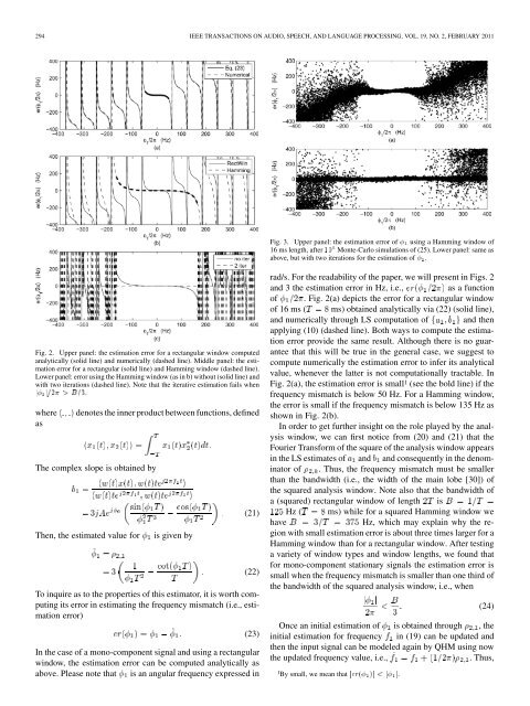
294 IEEE TRANSACTIONS ON AUDIO, SPEECH, AND LANGUAGE PROCESSING, VOL. 19, NO. 2, FEBRUARY 2011 Fig. 3. Upper panel: the estimation error of using a Hamming window of 16 ms length, after 10 Monte-Carlo simulations of (25). Lower panel: same as above, but with two iterations for the estimation of . Fig. 2. Upper panel: the estimation error for a rectangular window computed analytically (solid line) and numerically (dashed line). Middle panel: the estimation error for a rectangular (solid line) and Hamming window (dashed line). Lower panel: error using the Hamming window (as in b) without (solid line) and with two iterations (dashed line). Note that the iterative estimation fails when j j=2 > B=3. where as denotes the inner product between functions, defined The complex slope is obtained by Then, the estimated value for is given by (21) (22) To inquire as to the properties of this estimator, it is worth computing its error in estimating the frequency mismatch (i.e., estimation error) (23) In the case of a mono-component signal and using a rectangular window, the estimation error can be computed analytically as above. Please note that is an angular frequency expressed in rad/s. For the readability of the paper, we will present in Figs. 2 and 3 the estimation error in Hz, i.e., as a function of . Fig. 2(a) depicts the error for a rectangular window of 16 ms ( ms) obtained analytically via (22) (solid line), and numerically through LS computation of and then applying (10) (dashed line). Both ways to compute the estimation error provide the same result. Although there is no guarantee that this will be true in the general case, we suggest to compute numerically the estimation error to infer its analytical value, whenever the latter is not computationally tractable. In Fig. 2(a), the estimation error is small 1 (see the bold line) if the frequency mismatch is below 50 Hz. For a Hamming window, the error is small if the frequency mismatch is below 135 Hz as shown in Fig. 2(b). In order to get further insight on the role played by the analysis window, we can first notice from (20) and (21) that the Fourier Transform of the square of the analysis window appears in the LS estimates of and and consequently in the denominator of . Thus, the frequency mismatch must be smaller than the bandwidth (i.e., the width of the main lobe [30]) of the squared analysis window. Note also that the bandwidth of a (squared) rectangular window of length is Hz ( ms) while for a squared Hamming window we have Hz, which may explain why the region with small estimation error is about three times larger for a Hamming window than for a rectangular window. After testing a variety of window types and window lengths, we found that for mono-component stationary signals the estimation error is small when the frequency mismatch is smaller than one third of the bandwidth of the squared analysis window, i.e., when (24) Once an initial estimation of is obtained through , the initial estimation for frequency in (19) can be updated and then the input signal can be modeled again by QHM using now the updated frequency value, i.e., . Thus, 1 By small, we mean that jer( )j < j j.
Page 1 and 2: 290 IEEE TRANSACTIONS ON AUDIO, SPE
Page 3: 292 IEEE TRANSACTIONS ON AUDIO, SPE
Page 11: 300 IEEE TRANSACTIONS ON AUDIO, SPE

Adaptive AM–FM Signal Decomposition With Application to ... - ICS

Create successful ePaper yourself

Delete template?

Save as template?