Adaptive AM–FM Signal Decomposition With Application to ... - ICS

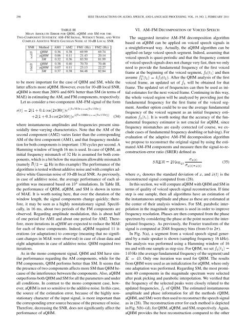
298 IEEE TRANSACTIONS ON AUDIO, SPEECH, AND LANGUAGE PROCESSING, VOL. 19, NO. 2, FEBRUARY 2011
TABLE III
MEAN ABSOLUTE ERROR FOR QHM, AQHM AND SM FOR THE
TWO-COMPONENT SYNTHETIC AM–FM SIGNAL, WITHOUT NOISE, AND WITH
COMPLEX ADDITIVE WHITE GAUSSIAN NOISE AT 10-dB LOCAL SNR.
to be more important for the case of QHM and SM, while the
latter affects more aQHM. However, even for 10-dB local SNR,
aQHM is more than 200% and 60% better than SM (in terms of
MAE) in estimating the AM, and FM components, respectively.
Let us consider a two component AM–FM signal of the form
(34)
where instantaneous amplitudes and frequencies present sinusoidally
time-varying characteristics. Note that the AM of the
second component (AM2) varies faster than the corresponding
AM of the first component (AM1), and that frequency modulation
for both components is important: 130 cycles per second. A
Hamming window of length 16 ms is used. In case of QHM, an
initial frequency mismatch of 32 Hz is assumed for both components,
which is a bit below the maximum allowable mismatch
(namely Hz in this example) The performance of the
algorithms is tested without additive noise and with complex additive
white Gaussian noise of 10-dB local SNR. As previously,
in case of additive noise, the average performance of each algorithm
was measured based on simulations. In Table III,
the performance of QHM, aQHM, and SM is shown in terms
of MAE. It is worth noting here, that over the duration of the
window length, the signal components change quickly; therefore,
it may be seen as a highly nonstationary signal. Specifically,
in 16 ms, about two periods of the FM components are
observed. Regarding amplitude modulation, this is about half
of one period for AM1 and about one period for AM2. Therefore,
more iterations in aQHM are expected to reduce the MAE
for each of these components. Indeed, aQHM required 11 iterations
(or adaptations) to converge (meaning that no significant
changes in MAE were observed) in case of clean data and
eight adaptations in case of additive noise. QHM required two
iterations.
As in the mono component signal, QHM and SM have similar
performance regarding the AM components, while for the
FM components, QHM performs better than SM. It seems that
the presence of two components affects more SM than QHM because
of the interference between the components. Also, aQHM
outperforms both QHM and SM for all the parameters and under
all conditions. In contrast to the mono component case, however,
aQHM is not so sensitive to the additive noise. In this case,
the source of the estimation error, because of the highly nonstationary
character of the input signal, is more important than
the corresponding error source because of the presence of noise.
Therefore, decreasing the SNR, does not significantly affect the
performance of aQHM.
VI. AM–FM DECOMPOSITION OF VOICED SPEECH
The suggested iterative AM–FM decomposition algorithm
based on aQHM can be applied on voiced speech signals in
a straightforward way. Actually, the aQHM algorithm can be
applied on large voiced speech segment. Indeed, assuming that
voiced speech is quasi-periodic and that the frequency content
of voiced speech signals does not change very fast, then we only
need to provide the fundamental frequency of the first voiced
frame at the beginning of the voiced segment, and then
assume
. After the QHM analysis of the first
voiced frame, an updated set of will be obtained for that
frame. The updated set of frequencies can then be used as initial
estimates for the next voiced frame. Continuing in this way,
the whole voiced region will be analyzed by providing just the
fundamental frequency for the first frame of the voiced segment.
Another option could be to use the average fundamental
frequency of the voiced segment as an initial frequency estimation
. It is worth noting that the accuracy of the fundamental
frequency estimator is not crucial for aQHM, since
frequency mismatches are easily corrected (of course, we exclude
cases of fundamental frequency doubling or halving). For
evaluation of the adaptive AM–FM decomposition algorithm
we propose to reconstruct the original signal by using the estimated
AM–FM components and measure then the signal-to-reconstruction-error
ratio (SRER) defined as
(35)
where denotes the standard deviation of , and is the
reconstructed signal computed from (28).
In this section, we will compare aQHM with QHM and SM in
terms of quality of voiced speech signal reconstruction. If time
step is one sample, then all algorithms have an estimation of
the instantaneous amplitude and phase as these are estimated at
the center of their analysis windows. For SM, parabolic interpolation
in the magnitude spectrum is used in order to improve
frequency resolution. Phases are then computed from the phase
spectrum by considering the phase at the point nearest the interpolated
frequency. As previously, the Fourier transform of the
signal is computed at 2048 frequency bins (from 0 to ).
In Fig. 5(a), a segment from a voiced speech signal generated
by a male speaker is shown (sampling frequency 16 kHz).
The analysis was performed using a Hamming window of 16
ms and with one sample as step size. For QHM, we set
Hz (the average fundamental frequency of the segment) and
. Only one iteration was used for QHM. The results
from QHM were used as an initialization for aQHM, where only
one adaptation was performed. Regarding SM, the most prominent
40 components in the magnitude spectrum were selected
after peak picking and parabolic interpolation. We verified that
the frequency of the selected peaks were closely related to the
updated frequencies, of QHM. The estimated instantaneous
amplitude and phase information for all the methods (QHM,
aQHM, and SM) were then used to reconstruct the speech signal
as in (28). The reconstruction error for each method is depicted
in Fig. 5(b)–(d), for QHM, aQHM, and SM, respectively. Again,
aQHM provides the best reconstruction compared to the other